Jul 13, 2004 - Division of Macro-Economic Statistics and Dissemination ... the academic literature to estimating hedonic price indexes. .... I would prefer an approach that only imputes 1. ~ .... period separately produces regression coefficients t α. ~ ... aggregate price index, based on a conventional index number formula.
Statistics Netherlands Division of Macro-Economic Statistics and Dissemination P.O.Box 4000 2270 JM Voorburg The Netherlands
Hedonic Regression: The Time Dummy Index As a Special Case of the Imputation Törnqvist Index
Jan de Haan
Project number: BPA number: Date:
Paper prepared for the eighth meeting of the International Working Group on Price Indices (Ottawa Group). The views expressed in this paper are those of the author and do not necessarily reflect the policies of Statistics Netherlands. I thank May Hua Oei for assistance. MOO-202862 -MOO 13 July 2004
HEDONIC REGRESSION: THE TIME DUMMY INDEX AS A SPECIAL CASE OF THE IMPUTATION TÖRNQVIST INDEX Abstract: This paper compares a Törnqvist price index in which the ‘missing prices’ are imputed using hedonic regression with the time dummy hedonic index. The aim is to show that the time dummy index can be interpreted as a special case of the imputation Törnqvist index when the regression weights are properly chosen. It is argued that the set of weights proposed in the recent literature overstates the impact of new and disappearing items. This could be particularly relevant for high-turnover goods like PCs. Keywords: consumer price index; hedonic imputation; time dummy index.
1. Introduction Silver and Heravi (2004) address the difference between hedonic imputation indexes and time dummy variable hedonic indexes, which are the two main approaches in the academic literature to estimating hedonic price indexes. The larger part of their paper relates to the imputation Törnqvist index and the time dummy index that uses the regression weights proposed by Diewert (2003). They analyse the factors driving the difference between both approaches and show that differences may arise from parameter instability and changes in the average characteristics and such differences are compounded when both occur. Their idea of looking at the time dummy variable model – which constrains the parameters to be the same across the two periods – as one that suffers from ‘omitted variable bias’ is particularly interesting. Silver and Heravi define imputation price indexes as indexes in which all prices are estimated using an hedonic model. That is, in addition to the imputation of ‘missing prices’ of new or disappearing items, observed prices are replaced by their predicted values. But throwing away observed prices is not an attractive idea, certainly not for statistical agencies. This paper therefore focuses on the partial imputation Törnqvist index in which hedonic imputation is restricted to ‘missing prices’. It is shown that the time dummy approach can be interpreted as a special case of the partial hedonic imputation Törnqvist index when the regression weights are properly chosen. The paper is organized as follows. Section 2 formally defines the partial imputation Törnqvist index. Section 3 shows that imputing ‘missing prices’ is essentially what a proper time dummy index does. Section 4 argues that the weights Diewert (2003) has suggested for the unmatched items in the estimation of the time dummy index are twice as large as they should be, at least if the partial imputation Törnqvist index serves as the preferred target index. Section 5 addresses some econometric issues. Section 6 provides empirical evidence using scanner data on personal computers for the Netherlands. Section 7 concludes. 1
2. The partial hedonic imputation Törnqvist index I start by introducing some notation. Let pi0 and pi1 denote the price of item i in the base period 0 and the current or comparison period 1, respectively, and let si0 and si1 denote the corresponding expenditure shares or relative sales values. Further, let S 0 and S 1 be the sets of models available in the respective periods. S M = S 0 ∩ S 1 denotes the set of matched items; S D0 is the set of disappearing items (those sold in period 0 but no longer in period 1) and S 1N the set of new items (those sold in period 1 but not in period 0). First I will define what I call the full hedonic imputation (FHI) geometric Laspeyres (GL) and geometric Paasche (GP) indexes. They can be written as
PFHIGL
0
æ = ∏ çç i∈I 0 è
si ~ æ pi1 ö ÷ ç = ∏ ~ ç pi0 ÷ø i∈S M è
æ = ∏ çç i∈S 1 è
si ~ æ pi1 ö ÷ = ∏ç 0 ÷ ~ ç pi ø i∈S M è
0
si ~ pi1 ö ÷ ~ pi0 ÷ø
0
æ ∏0 çç i∈S D è
si ~ p i1 ö ÷ , ~ p i0 ÷ø
si ~ æ pi1 ö ÷ ç 0 ÷ ∏ç ~ p i ø i∈S1N è
si ~ pi1 ö ÷ , ~ pi0 ÷ø
(1)
and
PFHIGP
1
1
1
(2)
where ~ pit denotes the predicted price of i in period t (t= 0,1), estimated with an hedonic model.1 Note that the prices in the expenditure shares are not replaced by their predicted values. Expressions (1) and (2) are generalized indexes in the sense that they incorporate all unmatched and matched items (see Diewert, 2003). There are two (related) problems with using those indexes. First, only in special circumstances will they coincide with the indexes based on observed prices when there are no unmatched items, depending on the specification of the model and the regression weights used. Second, statistical agencies may be reluctant to replace observed prices by predicted values, and to my pi1 for i ∈ S D0 opinion they are right. I would prefer an approach that only imputes ~ and ~ pi0 for i ∈ S 1N , leaving all observed prices unchanged, because this minimizes the impact of econometric modelling. This is what statistical agencies usually mean by imputation anyway.2 The partial hedonic imputation (PHI) geometric Laspeyres index and geometric Paasche index are given by
1
Triplett (2004) refers to this approach as the characteristics price index method since it uses the implicit characteristics prices (the regression coefficients from the hedonic function) in a conventional index number formula. Silver and Heravi (2004) call it the hedonic imputation method. This name may be confusing, so I termed it full hedonic imputation.
2
This idea is not new, of course. Triplett (2004) notes the following on the (partial) hedonic imputation method: “Where matched model comparisons are possible, they are used. Where they are not possible, a hedonic imputation is made for the item replacement. Hedonic imputation methods make maximum use of observed data, and minimum use of imputation, thereby minimizing estimation variance. The hedonic imputation method was employed in the hedonic computer indexes introduced into the U.S. national accounts in 1985”. Diewert (2003) also suggests matching items where possible and using hedonic regressions to impute the ‘missing prices’. 2
PPHIGL
æ p1 ö = ∏ çç i0 ÷÷ i∈S M è p i ø
si0
0
si æ~ p i1 ö ∏ çç 0 ÷÷ , i∈S D0 è p i ø
(3)
and
PPHIGP
æ p i1 ö = ∏ çç 0 ÷÷ i∈S M è p i ø
s1i
s1i
æ pi1 ö ∏1 çç ~p 0 ÷÷ . i∈S N è i ø
(4)
Taking the geometric average of (3) and (4) leads to the partial hedonic imputation Törnqvist index:
PPHIT =
æp ö ÷÷ i∈S M è ø
∏ çç p
1 i 0 i
si0 + s1i 2
æ
∏ çç
i∈S D0
è
si0
~ pi1 ö 2 ÷ pi0 ÷ø
s1i 2
æp ö ÷÷ . i∈S 1N è ø
∏ çç ~p
1 i 0 i
(5)
I prefer PPHIT as the (geometric) target index because it is a generalized superlative index that restricts hedonic imputation to the ‘missing prices’.3 Diewert (2003) argues that the residuals from a logarithmic hedonic model are less likely to be heteroskedastic than those from a linear model. Most empirical studies seem to prefer the logarithmic specification as well. For period t (t= 0,1) the semilog (log-linear) model regression can be expressed as K
ln pit = α t + å β kt z ik + ε it ,
(6)
k =1
where z ik is the k-th characteristic of item i and β kt the corresponding parameter; the errors ε it are assumed to be independently distributed with expected values of zero and constant variances. Least squares estimation of (6) on the data from each ~ period separately produces regression coefficients α~ t and β kt and predicted prices K ~ ~ pit = exp(α~ t + k =1 β kt z ik ) .4
å
3. The time dummy index The second main approach to estimating hedonic price indexes is the time dummy variable method. In this case the cross section data from period 0 and period 1 are pooled. The semi-log hedonic model reads K
ln pit = α + δDit + å β k z ik + ε it ,
(7)
k =1
3
See De Haan (2004a) for a double imputation hedonic geometric index in which period 0 and period 1 prices are imputed for both new and disappearing items (but not for matched items). De Haan (2002) calls the partial imputation Fisher index a generalized Fisher index.
4
The predictors are not unbiased estimators of the actual prices. Van Dalen and Bode (2004) evaluate the biases in various hedonic indexes due to the use of a logarithmic hedonic model. 3
where Dit is a dummy variable that takes on the value of 1 if the observation comes from period 1 and 0 otherwise. The errors ε it are now assumed to be similarly and independently distributed in both periods, which may be rather restrictive. Model (7) assumes that each of the characteristics parameters is the same across the two time periods compared, i.e. β k0 = β k1 = β k for k=1,….,K by assumption. As (7) controls for changes in the quality characteristics, the exponent of the estimated time dummy coefficient δˆ directly produces a quality-adjusted measure of price change. The K predicted prices in period 0 and period t are denoted pˆ i0 = exp(αˆ + k =1 βˆ k z ik ) K and pˆ i1 = exp(αˆ + δˆ + k =1 βˆ k z ik ) . Note that pˆ i1 / pˆ i0 = exp δˆ for all i.
å
å
We may ask the question under what circumstances exp δˆ can be interpreted as an aggregate price index, based on a conventional index number formula. Silver (2003) criticises the use of Ordinary Least Squares (OLS) to estimate (7). The observations should be weighted according to their economic importance. Thus, a certain type of Weighted Least Squares (WLS) should be used. Van der Grient and De Haan (2003) present a decomposition of the WLS time dummy index which I will repeat here and extend for further analysis. Let wi0 and wi1 denote the regression weights for i ∈ S 0 and i ∈ S 1 , respectively. That is, each observation in period t counts wit times in the estimation procedure. Because a constant term is included in (7), the residuals sum to zero in each period and the following relation holds:
æ p i0 ö ç 0÷ ∏ ç ˆ ÷ i∈S M è p i ø
wi0
æ pi0 ö ∏0 çç pˆ 0 ÷÷ i∈S D è i ø
wi0
æ pi1 ö = ∏ çç 1 ÷÷ ˆi ø i∈S M è p
w1i
w1i
æ p i1 ö ∏1 çç pˆ 1 ÷÷ (= 1) . i∈S N è i ø
(8)
Some rearranging and subsequently substituting pˆ i1 / pˆ i0 = exp δˆ for i ∈ S M leads to a decomposition of the WLS time dummy index:
PTD = exp δˆ = where w1M =
æp ö ÷÷ i∈S M è ø
∏ çç p
å
i∈S M
1 i 0 i
w1i w1M
æp ö ÷÷ i∈S M è ø
∏ çç pˆ
0 i 0 i
w1i − wi0 w1M
æp ö ÷÷ i∈S D0 è ø
∏ çç pˆ
0 i 0 i
− wi0 w1M
æp ö ÷÷ i∈S 1N è ø
∏ çç pˆ
1 i 1 i
w1i w1M
,
(9)
wi1 .
Van der Grient and De Haan (2003) formulate two requirements equation (9) should satisfy. The first requirement is that the resulting index should be based on observed prices when there are no new or disappearing items. Quality changes do not occur in that case, although the quality mix may change because of changes in the quantities sold, and we want the outcome to be independent of the set of characteristics. The second factor of (9) contains the period 0 residuals of the matched items and usually differs from unity. Hence, the first requirement will not be met. We therefore impose the restriction wi0 = wi1 = wi (independent of time) for i ∈ S M , which assures that wi / wM ( pi1 / p i0 ) , the time dummy index equals the matched-item index PM = i∈S M 5 where wM = i∈S wi , when there are only matched items. This yields
å
∏
M
5
This restriction does not hold if there is no weighting of the observations involved (OLS), unless the number of observations is constant over time (e.g., under the fixed-size sampling 4
PTD ( R ) =
æp ö ÷÷ i∈S M è ø
∏ çç p
1 i 0 i
wi wM
æp ö ÷÷ i∈S D0 è ø
∏ çç pˆ
0 i 0 i
− wi0 wM
æp ö ÷÷ i∈S 1N è ø
∏ çç pˆ
1 i 1 i
w1i wM
.
(10)
Equation (10) shows an important property of the time dummy index satisfying the above restriction: it can be viewed as an index where all observed prices, including those of the unmatched items, are kept and not replaced by their predicted values. This is in line with the partial hedonic imputation indexes defined in section 2. What I did not realize before was that, by using pˆ i1 / pˆ i0 = exp δˆ for i ∈ S D0 and i ∈ S 1N , equation (10) can be rewritten as wi é æ p 1 ö wi æ pˆ i1 ö i = ê ∏ çç 0 ÷÷ ∏ çç 0 ÷÷ êi∈S M è pi ø i∈S D0 è pi ø ë
0
PTD ( R )
å
1
æp ö ÷ ÷ 1 i∈S N è ø
∏ çç pˆ
1 i 0 i
wi1
ù wM + wD0 + w1N ú , ú û
(11)
å
where wD0 = i∈S 0 wi0 and w1N = i∈S 1 wi1 . Notice that the term between square D N brackets has the same structure as PPHIT given by (5). The time dummy index (11) can also be written as a weighted geometric mean of the matched-model index PM defined above and hedonic imputation indexes for disappearing and new items:
PTD ( R ) = [PM ] where PˆD =
wM wM + wD0 + w1N
∏
i∈S D0
[ ] PˆD
wD0
wM + wD0 + w1N 0
( pˆ i1 / pi0 ) wi
wD0
[ ] PˆN
w1N
wM + wD0 + w1N
and PˆN =
∏
,
i∈S 1N
(11’) 1
( pi1 / pˆ i0 ) wi
w1N
.
A second requirement is that the resulting index number formula can be defended on theoretical grounds. This implies that the price relatives must somehow be weighted by expenditure shares.6 The use of OLS is no longer an option unless we are dealing with fixed-size sets of items sampled proportional to expenditure (De Haan, 2003). The choice of regression weights is explored in section 4.
4. Choice of weights For the matched items we have expenditure shares of both period 0 and period 1. For reasons of symmetry their unweighted arithmetic average is a natural choice, which also meets the first requirement. This choice has been suggested by Diewert (2003); the time dummy index would then equal the superlative Törnqvist index when there are only matched items. Substituting wi = ( s i0 + s i1 ) / 2 for i ∈ S M into (11) yields the (pseudo) generalized Törnqvist index
schemes applied by most statistical agencies). Yet the use of OLS always satisfies the first requirement: it produces the unweighted geometric index when all items are matched. 6
Various authors, for example Silver and Heravi (2002) and Van Mulligen (2003), have used the quantities sold in the respective periods as weights in the WLS estimation of time dummy indexes. This procedure violates both requirements and should be adviced against. 5
si + s i é 1 2 æ ö p ê = ê ∏ çç i0 ÷÷ p êi∈S M è i ø ë 0
~ PTD ( GT )
1
1
æ pˆ i1 ö ∏0 çç p 0 ÷÷ i∈S D è i ø
wi0
æ pi1 ö ∏ çç ˆ 0 ÷÷ i∈S 1N è p i ø
w1i
ù sM0 + s1M + wD0 + w1N ú 2 , ú ú û
å
(12)
å
using wM = ( s M0 + s 1M ) / 2 , where s M0 = i∈S s i0 and s 1M = i∈S s i1 denote the M M matched items expenditure shares in period 0 and period 1, respectively. For the unmatched items the choice of weights is less obvious. I propose to take half the expenditure shares in the periods they are available, i.e. wi0 = s i0 / 2 for i ∈ S D0 and wi1 = si1 / 2 for i ∈ S 1N . Substituting those weights into (12) gives
PTD ( H ) =
æp ö ÷÷ i∈S M è ø
∏ çç p
1 i 0 i
si0 + s1i 2
æ pˆ ö ÷÷ 0 i∈S D è ø
∏ çç p
1 i 0 i
si0 2
s1i 2
æp ö ÷÷ , 1 i∈S N è ø
∏ çç pˆ
1 i 0 i
(13)
since now wD0 = (1 − s M0 ) / 2 and w1N = (1 − s 1M ) / 2 , so that wM + wD0 + w1N = 1 . Expression (13) is similar to (5). Thus, using the proposed weights, the time dummy index is a special case of the partial hedonic imputation Törnqvist price index (5) in which the ‘missing prices’ are automatically imputed according to the time dummy variable model (7). Notice that the regression weights are identical to the weights used to aggregate the price relatives. De Haan (2004a) also applies (7) in a hedonic imputation approach and refers to this as an indirect time dummy approach. In the special case discussed here the direct and indirect approaches coincide. This seems a desirable property. Diewert (2003), on the other hand, suggests taking the full expenditure shares of the unmatched items as regression weights. His suggestion has been followed by Silver and Heravi (2004) and also by Van der Grient and De Haan (2003), Van der Grient (2004), and De Haan (2004b) – it is mentioned in the new CPI manual (ILO, 2004) as well.7 Substituting wi0 = s i0 for i ∈ S D0 and wi1 = s i1 for i ∈ S 1N into (12) yields si + si é 1 2 æ ö p ê = ê ∏ çç i0 ÷÷ p êi∈S M è i ø ë 0
PTD ( D )
1
2
ù 4− sM0 − s1M ú ú ú û
4
0 si ù 4 − s M − s1M é 1 2 ê æç pˆ i ö÷ ú ê∏0 ç p 0 ÷ ú êi∈S D è i ø ú û ë 0
4
0 si ù 4 − s M − s1M é 1 2 ê æç pi ö÷ ú . (14) ê∏1 ç pˆ 0 ÷ ú i∈S N è i ø ú ê û ë 1
I find it difficult to justify this choice of weights since expression (14) has no clear interpretation as a generalized Törnqvist index. The weight of the matched items is understated and the weights of new and disappearing items overstated. The overall impact depends on the imputed prices of the unmatched items, which will naturally differ using different weights. However, if the model specification is satisfactory, then we may expect this effect to be relatively small compared to the effect of the ‘wrong’ weights with which the price relatives are implicitly aggregated.
7
See Silver (2003) for a general discussion on the use of weights. 6
Now that we have determined the optimal regression weights, various expressions or decompositions of the time dummy index can be derived in order to provide further insight. For example, equation (13) can be rewritten in the form of (11’), yielding
é 0 1 1 ê æç pi ö÷ sM + sM = ê∏ ç 0 ÷ p êi∈S M è i ø ë si0 + s1i
PTD ( H )
ù ú ú ú û
0 sM + s1M 2
∏
0 1− s M 2
[PDGL ] 0
1− s1M 2
[PNGP ]
,
(15)
∏
0
1
1
( pˆ i1 / pi0 ) si (1− sM ) and PNGP = i∈S 1 ( pi1 / pˆ i0 ) si (1− sM ) are where PDGL = i∈S D0 N the hedonic imputation geometric Laspeyres index and geometric Paasche index for disappearing items and new items, where the imputations are based on model (7). A second and perhaps more convenient decomposition results from substituting the proposed weights into (10). Denoting the regression residuals ln p it − ln pˆ it by u it and the expenditure share weighted average residuals of new and disappearing items by u N1 = i∈S 1 si1u i1 / i∈S 1 s i1 and u D0 = i∈S 0 si0 u i0 / i∈S 0 s i0 , we obtain
å
PTD ( H ) =
å
N
æp ö ÷ ÷ i∈S M è ø
∏ çç p
1 i 0 i
si0 + s1i 0 sM + s1M
å
N
1− s1M 1 0 s M + s1M N
[exp u ] [exp u ]
0 1− s M 0 0 s + s1 D M M
.
D
å
D
(16)
Under perfect competition u D0 and u N1 are likely to approximate zero. The so-called law of one quality-adjusted price predicts that there will be no items whose prices are relatively high or low given their characteristics: there should be no ‘unusual’ prices. Equation (16) shows that the time dummy index will then be approximately 0 1 0 1 ( pi1 / pi0 ) ( si + si ) /( sM + sM ) . But under imperfect equal to the matched-item index i∈S M competition there are economic reasons to expect that such unusual prices will exist (Silver and Heravi, 2002; Triplett, 2004).
∏
5. Econometric considerations Because the time dummy index (13) is a special case of the broader class of (partial) imputation Törnqvist indexes, one could argue that it would be better to estimate the ‘missing prices’ explicitly, based on econometric arguments, rather than implicitly as the time dummy index does. From an econometric point of view, there are again the issues of pooling data and weighting. Pooling data is of course not necessary for an imputation approach. The assumption of constant parameters is rather stringent, and estimating (log-linear) hedonic models from data of each period separately would in principle be best. Indeed, this has been suggested in section 2 and it is also what Silver and Heravi (2004) do in the estimation of the full hedonic imputation indexes. But pooling data has two advantages. First, there is an expected gain in efficiency by saving degrees of freedom, which can be particularly helpful when the sample size is relatively small. Second, it makes the estimation of period 0 prices possible for new
7
items having characteristics that did not exist at that time. Moreover, although the underlying assumption is restrictive in theory, many if not most empirical studies find the parameters to be fairly stable in the short run. Let us compare the proposed time dummy index with the partial hedonic imputation Törnqvist index estimated on data from each period separately. Dividing (13) by (5) and substituting the expressions for the unmatched items’ predicted prices gives
PTD ( H ) PPHIT
=
(
)
é ì ~ 1 0 üù ˆ ~1 ˆ êexpíαˆ + δ − α + å β k − β k z Dk ýú k =1 þû ë î K
(
)
K é ì ~ üù ~0 + ˆ − α α β k0 − βˆ k z 1Nk ýú exp å ê í k =1 þû ë î
å
å
[ { (
)}]
0 1− s M 2
1− s1M 2
å
,
(17)
å
0 = i∈S 0 s i0 z ik / i∈S 0 s i0 and z 1Nk = i∈S1 s i1 z ik / i∈S 1 s i1 denote the where z Dk D D N N expenditure-weighted average characteristics of disappearing and new items. If the assumption of constant characteristics parameters (approximately) holds, we expect ~ ~ to find βˆ k ≈ β k0 ≈ β k1 . For simplicity I assume that s 1M ≈ s M0 . Now (17) reduces to
PTD ( H ) PPHIT
≈ exp δˆ − α~ 1 − α~ 0
0 1− s M 2
.
(18)
Expression (18) does not seem helpful at first sight because the time dummy index PTD ( H ) = exp δˆ appears on the right-hand side. However, it underlines the fact that, from an imputation point of view, δ in (7) is viewed as a common shift parameter needed to justify the pooling of data from two data sets, pertaining to two periods, under the assumptions of constant characteristics parameters and independently and identically distributed errors. Stated otherwise, under these assumptions δˆ is merely an estimator of α 1 − α 0 , and PTD ( H ) is likely to differ only marginally from PPHIT . PTD ( H ) is the more efficient estimator due to the pooling of data. The choice of weights has to do with representativity. The chosen weights – or any other set of weights for that matter – may not be optimal from an econometric point of view. Econometrics textbooks recommend the use of WLS to reduce the variance of the coefficients if there is evidence of heteroskedasticity. On the other hand, if the errors are homoskedastic (as assumed), OLS is preferred in general and WLS could introduce some loss in efficiency.8 That would partly compensate the efficiency gain resulting from the pooling of data. The problem is of course that by using OLS to estimate model (7) on the pooled data we are ‘running around in circles’ because the similarity between the (direct) time dummy approach and the imputation Törnqvist index (the ‘indirect’ time dummy approach) no longer holds. To avoid interpretation problems, the proposed time dummy index might well be the only serious option if 8
If the weights are exogenous, least squares estimators remain unbiased. The weights are not truly exogenous since they contain the dependent variable (price) of the model, which makes them stochastic variables. This could introduce some bias in the WLS estimators. 8
one wishes to pool cross-section data to estimate a quality-adjusted price index using a logarithmic hedonic model. The time dummy index essentially imputes ‘missing prices’. As with any imputation method, we have to act as if the data had been generated by the underlying model. In this particular case it is assumed that the (log of) prices are generated according to model (7). One issue I mentioned earlier (De Haan, 2003, 2004a; Van der Grient and De Haan, 2003) keeps bothering me. Suppose we find empirically that the weighted average residuals of the unmatched items in expression (16) differ substantially from zero. If the number of unmatched items is sufficiently large, this could be taken as evidence of systematic patterns in the unmatched items’ residuals. This suggests that the assumption of a zero expected value of the errors is violated, so that estimating (7) by least squares regression produces biased parameter estimators. Isn’t there an inconsistency in assuming that the (log of) prices are generated according to model (7) and at the same time finding that the observed (log of) prices of the unmatched items differ systematically from their model-based predictions? De Haan (2003) has argued that the direct time dummy approach cannot cope with such systematic price effects of unmatched items and suggested to incorporate dummy variables for those items. But that is beyond the scope of this paper.
6. Empirical illustration: PCs The effect of the use of the ‘wrong’ regression weights on the time dummy index is an empirical matter. This section presents empirical evidence for PCs using scanner data from market research company GfK. The monthly data on prices (unit values), quantities sold and product characteristics cover the entire Dutch consumer market during 1999-2001. A comprehensive data description can be found in Van der Grient (2004). Individual PC models are usually identified by model numbers or, as in our case, by bar codes assigned by the manufacturers. A specific model sold in different outlets does not necessarily yield the same utility to the consumer. PCs having identical bar codes but sold in different types of outlets are therefore treated as different items. Six outlet types are distinguished in the data set, e.g. chains, buying combinations, independents, and specialized stores. The latter are responsible for the greater part of PCs sales. The market for PCS is an extremely dynamic one. On average only two thirds of the items are matched between adjacent months. Because the best selling items have a relatively long ‘lifetime’, the average monthly expenditure share of the matched items is somewhat higher and amounts to 0.8. To give an example: only 5% of the items stay on the market for more than a year, but they account for 30% of total turnover. New PC models often have new features, e.g. a ‘faster’ processor. The time dummy index deals with this by estimating and imputing base period prices for such models. This poses theoretical problems, however, if the new technology was not available 9
in the base period. This will be particularly problematic when the base period and the current period are far apart. Apart from that, it seems undesirable to maintain the assumption of constant parameters for a long time span in highly dynamic markets. High-frequency chaining is inevitable here. So unlike Silver and Heravi (2004), who compute direct indexes, I will estimate monthly chained indexes. This may not be without problems either because PC sales exhibit a seasonal pattern.9 As is well known, seasonality might create drift in monthly-chained indexes. The semi-log time dummy models include dummy variables for both brand and type of outlet. See De Haan (2004b) for some (OLS) regression results. Most coefficients differ significantly from zero at the 5%-level and their signs are in accordance with a priori expectations. No evidence of heteroskedasticity was found. The adjusted R 2 does not exceed 0.71, which is rather disappointing. This may be due to the fact that only a limited number of technical or performance characteristics, such as type of processor and availability of a monitor, are available in the data set. Unobserved relevant characteristics could give rise to omitted variables bias.
110 100 90 80 70 60 50 40
TDI; proposed weights Matched-item Törnqvist
200111
200109
200107
200105
200103
200101
200011
200009
200007
200005
200003
200001
199911
199909
199907
199905
199903
199901
30
TDI; 'wrong' weights TDI; OLS
Figure 1. Monthly chained price indexes for PCs (January 1999= 100) Figure 1 depicts four series of monthly-chained price indexes. The first two series pertain to WLS time dummy hedonic indexes, estimated with the proposed weights and the weights suggested by Diewert (2003), respectively. The third series pertains to the OLS time dummy index and the fourth series to the matched-item Törnqvist 0 1 1 0 ( siM + siM ) / 2 t ( p i / pi ) , where siM is the share of i in the period t index PMT = i∈S M expenditures of the matched-items. The latter two series are added for comparison.
∏
9
This is true at the aggregate level. However, since most models are available on the market for less than a year, it is difficult to speak of seasonality at the level of individual items. 10
All indexes have similar trends and point towards large declines in quality-adjusted PC prices, as expected. The time dummy index estimated with the ‘wrong’ weights falls at a faster rate than the proposed time dummy index, although the difference is very small compared to the huge price decrease itself. In January 2002 the index numbers are 31.84 and 34.57. This result indicates that new and disappearing items had a combined downward effect on the quality-adjusted index. The use of the matched-item Törnqvist index would have led to an annual average upward bias of 1.5%-points during the three-year period. Surprisingly, the OLS time dummy index, despite being an unweighted index, performs quite well.
7. Conclusion Using a simple framework this paper argues that the time dummy hedonic index can be interpreted as a special case of the hedonic imputation Törnqvist price index if the regression weights are properly chosen. The weights for the unmatched (new and disappearing) items suggested in the recent literature on hedonics are twice as large as they should be if the aim is to estimate a generalized Törnqvist index. The choice of weights most likely affects the index for high-turnover goods like computers. An empirical illustration on scanner data for the Netherlands indicated that the use of the ‘wrong’ weights would have underestimated the monthly chained time dummy index for PCs during 1999 – 2001 by some 2.7 index points.
References Dalen, J. van, and B. Bode, 2004, Estimation Biases in Quality-Adjusted Hedonic Price Indices, Paper presented at the SSHRC International Conference on Index Number Theory and the Measurement of Prices and Productivity, Vancouver, June 30 – July 3, 2004. Diewert, W.E., 2003, Hedonic Regressions: A Review of Some Unresolved Issues, Proceedings of the Seventh Meeting of the International Working Group on Price Indices, (ed. Th. Lacroix), pp. 71-109. Paris: INSEE. Grient, H.A. van der, 2004, Scanner Data on Durable Goods: Market Dynamics and Hedonic Time Dummy Indexes, Mimeo, Statistics Netherlands, Voorburg. Grient, H.A. van der, and J. de Haan, 2003, An Almost Ideal Hedonic Price Index for Televisions, Proceedings of the Seventh Meeting of the International Working Group on Price Indices, (ed. Th. Lacroix), pp. 111-121. Paris: INSEE. Haan, J. de, 2002, Generalised Fisher Price Indexes and the Use of Scanner Data in the CPI, Journal of Official Statistics, 18, vol. 1, 61-85.
11
Haan, J. de, 2004a, Direct and Indirect Time Dummy Approaches to Hedonic Price Measurement, Journal of Economic and Social Measurement (forthcoming). Haan, J. de, 2004b, Estimating Quality-Adjusted Unit Value Indexes: Evidence from Scanner Data, Paper presented at the SSHRC International Conference on Index Number Theory and the Measurement of Prices and Productivity, Vancouver, June 30 – July 3, 2004. International Labour Office (ILO), 2004, Consumer Price Index Manual; Theory and Practice. Geneva: ILO Publications. Mulligen, P.H. van, 2003, Quality Aspects in Price Indices and International Comparisons: Applications of the Hedonic Method, Ph.D. Dissertation, University of Groningen. Voorburg: Statistics Netherlands. Silver, M., 2003, The Use of Weights in Hedonic Regressions: The Measurement of Quality-Adjusted Price Changes, Proceedings of the Seventh Meeting of the International Working Group on Price Indices, (ed. Th. Lacroix), pp. 135-147. Paris: INSEE. Silver, M. and S. Heravi, 2002, Why the CPI Matched Models Method May Fail Us: Results from an Hedonic and Matched Experiment Using Scanner Data, European Central Bank (ECB) Working Paper No. 144, ECB, Frankfurt. Silver, M. and S. Heravi, 2004, The Difference between Hedonic Imputation Indexes and Time Dummy Hedonic Indexes for Desktop PCs, Paper presented at the CRIW Conference on Price Index Concepts and Measurement, Vancouver, June 28-29, 2004. Triplett, J.E., 2004, Handbook on Hedonic Indexes and Quality Adjustments in Price Indexes (Draft, June 2004). Paris: Organization for Economic Co-operation and Development.
12