Peter J. Rousseeuw is Professor and Mia Hubert is Assistant, Department of Mathematics and Computer ..... In (Hubert and Rousseeuw 1997) an efficient O(nlogn) algorithm is constructed to ...... York: Chapman and Hall. ... York: John Wiley.
Regression Depth Peter J. Rousseeuw and Mia Hubert
�
Second Revision, 4 May 1998
Abstract In this paper we introduce a notion of depth in the regression setting. It provides the `rank' of any line (plane), rather than ranks of observations or residuals. In simple regression we can compute the depth of any line by a fast algorithm. For any bivariate data set Zn of size n there exists a line with depth at least n=3. The largest depth in Zn can be used as a measure of linearity versus convexity. In both simple and multiple regression we introduce the deepest fit, which generalizes the univariate median and is equivariant for monotone transformations of the response. Throughout, the errors may be skewed and heteroskedastic. We also consider depth-based regression quantiles. They estimate the quantiles of y given x, as do the Koenker-Bassett regression quantiles, but with the advantage of being robust to leverage outliers. We explore the analogies between depth in regression and in location, where Tukey's halfspace depth is a special case of our general definition. Also Liu's simplicial depth can be extended to the regression framework.
KEY WORDS: Asymmetric error distribution; Deepest fit; Depth envelopes; Depth quantiles; Geometry; Halfspace depth; Robust regression; Simplicial depth.
Peter J. Rousseeuw is Professor and Mia Hubert is Assistant, Department of Mathematics and Computer Science, Universitaire Instelling Antwerpen (UIA), Universiteitsplein 1, B-2610 Wilrijk, Belgium. We would like to thank Anja Struyf and Stefan Van Aelst for computational assistance. We are grateful to the Editor, Associate Editor, and three referees for comments which improved the presentation. �
1 Introduction In this paper we propose the notion of regression depth. We view depth as a property of a t (typically determined by a vector � of coefficients), rather than a property of an observation. In general we define the depth of a (candidate) fit � to a given data set Zn of size n as
Definition 1. The depth(�; Zn) is the smallest number of observations of Zn that would need to be removed in order to make � a non t.
Therefore, always 0 � depth(�; Zn) � n. (In the population case, we ask how much probability mass needs to be removed.) A particular depth function is thus equivalent to the definition of a nonfit (since nonfits are exactly those fits with zero depth). Section 2 defines nonfits in simple regression, and constructs a fast algorithm for computing the regression depth of a line. We show that the largest regression depth relative to a data set Zn is at least n=3, by constructing a line which is at least that deep. The maximal depth of Zn is at its highest when the linear model holds well, and at its lowest when the data lie on a parabola or any other curve which is strictly convex or concave. The maximal regression depth thus reflects the degree of linearity in the data. We then consider the deepest line (that is, with largest regression depth), which generalizes the univariate median. The deepest line has a breakdown value of 1=3. Around that line we construct depth envelopes, which are useful for graphical display. Section 3 defines regression depth in the multiple regression setting with p coefficients, with the corresponding deepest fit and depth envelopes. The breakdown value of the deepest fit approaches 1/3 in any dimension. Due to the monotone invariance of regression depth, the deepest fit is equivariant to monotone transformations of the response, unlike least squares, least absolute values (L ) or least median of squares. Throughout the paper, the errors may be skewed and non-identically distributed (e.g. heteroskedastic). In Section 4 we consider depth-based regression quantiles. They estimate the conditional quantile of y given x, as do the customary L -based regression quantiles of Koenker and Bassett (1978), but with the additional advantage of being robust to leverage outliers. Section 5 gives another interpretation of regression depth, using duality. For bivariate data the dual plot represents observations as lines, and candidate fits as points. This yields some interesting insights, and new results of geometry. Section 6 focuses on the multivariate location setting. By applying Definition 1 we 1
1
1
recover the (halfspace) location depth of Tukey (1975) as a special case. This location depth has been used as a multivariate generalization of rank. The deepest location (Donoho and Gasko 1992) also generalizes the univariate median, and its depth reflects the degree of angular symmetry in the data. Interestingly, it turns out that (under additional conditions) both types of depth have precursors in the fifties, since simple regression depth is related to a test of Daniels (1954) in exactly the same way that bivariate location depth is related to a test of Hodges (1955). Section 7 explains how Liu's simplicial depth (1990) for location can be extended to the regression context. Both the deepest fit and L regression are generalizations of the univariate median. Section 8 argues that the deepest fit is the more natural one, and also compares it with least median of squares. Section 9 describes some directions for further research. 1
2 Simple regression 2.1 Definition of regression depth In simple regression we want to fit a straight line y = � x + � to a data set Zn = f(xi; yi); i = 1; : : : ; ng � R . All candidate fits will be denoted as � = (� ; � ) so the first component is the slope estimate and the second is the intercept term. The residuals are then denoted as ri (�) = ri = yi ? � xi ? � . 1
2
2
1
1
2
2
Definition 2. A candidate t � = (� ; � ) to Zn will be called a non t i� there exists a real 1
2
number v� = v which does not coincide with any xi and such that or
ri(�) < 0
for all xi < v
and
ri (�) > 0
for all xi > v
ri(�) > 0
for all xi < v
and
ri(�) < 0
for all xi > v:
Figure 1 shows a data set with 6 observations and two nonfits � and �. Also the corresponding values v� and v� are indicated. From this plot it is clear that the existence of v corresponds to the presence of a tilting point (marked by a cross) around which we can rotate the line until it is vertical, while not passing any observation. Note that a line lying above or below all the observations (such as the line �) is always a nonfit. The notion of regression depth now follows immediately from the general concept of depth (Definition 1): 2
θ
y
4•
ξ
•5
1•
•
3
2•
•6
η
vη
vθ
x
Figure 1: Bivariate data set with two non ts � and �, and a t � with regression depth 2.
Definition 3. The regression depth of a t � relative to a data set Zn is the smallest number
of observations that need to be removed to make � a non t. Equivalently, rdepth(�; Zn ) is the smallest number of residuals that need to change sign.
For example, consider the line � in Figure 1. We can make it a nonfit by removing observations 4 and 5 (since one can then tilt � vertically without touching any remaining observations, e.g. using v� ). Since � cannot be made a nonfit by removing fewer observations, rdepth(�; Zn) = 2. Note that Definitions 2 and 3 allow for ties among the xi and that they do not require any distributional assumptions. To compute rdepth(�; Zn) we first reorder the observations such that x � x � : : : � xn in O(n log n) time. Then we can compute the depth in O(n) operations using 1
2
rdepth(�; Zn) = min (minfL (xi) + R?(xi ); R (xi) + L? (xi)g) �i�n +
+
1
where
(2.1)
L (v) = #fj ; xj � v and rj � 0g; R?(v) = #fj ; xj > v and rj � 0g; +
and L? and R are defined accordingly. It therefore suffices to update L (xi ), L? (xi), R? (xi) and R (xi ) at each i = 1; : : : ; n. +
+
+
3
From Definition 3 it follows that regression depth is scale invariant, regression invariant and affine invariant, according to the definitions in Rousseeuw and Leroy (1987, page 116). In the population case rdepth(�; H ) is defined as the smallest probability mass that has to be removed, where H is the joint distribution of the (x; y).
2.2 The maximal depth Definition 3 implies that the rdepth of any fit is at most n. This upper bound is reached if all the (xi; yi) lie exactly on a straight line. In general the maximal depth will be lower. Theorem 1 establishes lower and upper bounds for the maximal regression depth.
Theorem 1. (a) At any data set Zn � R it holds that 2
lnm max rdepth ( � ; Z ) � n � 3 where the ceiling d�e is the smallest integer � �. (b) If the (xi ; yi) are in general position, i.e., no three (xi ; yi ) lie on a line, �
�
n+2 : max rdepth ( � ; Z ) � n � 2 (c) For any (x; y)-distribution H on R with a density it holds that 1 � max rdepth(�; H ) � 1 : � 3 2 (d) If H has a density and satis es
(2.2)
(2.3)
2
med(y ? �~ x ? �~ jx = x ) = 0 1
2
0
for all x0 2 R
(2.4)
(2.5)
for some �~ = (�~1 ; �~2 ) 2 R 2 then
~; H ) = 1 : max rdepth ( � ; H ) = rdepth ( � (2.6) � 2 Condition (2.5) is very weak, e.g. it does not require that the conditional distribution of (y ? �~ x ? �~ )jx = x be symmetric, or that it stays the same across different values of x . Note that our functional form is parametric whereas the error distribution is nonparametric, so we have a semiparametric model. This model is very large and allows for skewness and heteroskedasticity, which often occur in practice. Theorem 2 shows when the lower bounds in Theorem 1 are reached. 1
2
0
0
4
Theorem 2. (a) If all xi are distinct and the (xi ; yi) lie on a strictly convex (or strictly concave) curve, then
�
�
n+2 : max rdepth ( � ; Z ) = n � 3 (b) If the probability mass of H is concentrated on a strictly convex (or concave) curve, then 1: max rdepth ( � ; H ) = � 3 From Theorems 1 and 2 it follows that max� rdepth(�; Zn) can be seen as a measure of linearity for Zn. Note that this quantity can be computed in O(n ) time from 3
max rdepth(�; Zn) = max rdepth(�ij ; Zn) i 0 for all xi in one of its open halfspaces, and ri(�) < 0 for all xi in the other open halfspace. 1
10
100%
4 93%
79%
• 2000
Recruits
4000
6000
8000
(a)
7
• 10
0
•
• • • • •
•
• • •
••
••
•
•
••
•
•
•
•
• •
61%
Tr*
36%
•• 11%
10 7 -2000
0%
4 0
200
400
600
800
1000
1200
Spawners
100
(b)
80
• •
%
60
•
40
•
•
••
•
20 0
• •• 40
•
00 Re
•
•
• ••
•
• 00
•
•
•
60
•
••
••
•
0
20
0 cru 0 its
800 0
400 200
-2
00
0
100
600 ers awn
Sp
0
Figure 4: (a) The Skeena River data set (n = 28), its deepest line Tr� (with depth 12) and its depth envelopes for k = 4, 7 and 10. To the left of each envelope boundary its value of k is listed, and to its right the (cumulative) percentage of the data lying on or below it; (b) terrace plot of the depth envelope boundaries, with the percentages on the vertical axis.
11
An example of a nonfit is shown in Figure 5. Here p = 3, so � corresponds to a plane. The x-space can be seen as the horizontal plane given by y � 0, which contains the line V . (By definition, any �0 with all ri(�0) > 0 or all ri(�0 ) < 0 is also a nonfit, since it then suffices to choose V such that all xi lie on the same side of V .)
y + +
+ +
+
+
+
θ -
-
-
x2
-
V x1
Figure 5: An example of a non t � 2 R 3 . The a�ne hyperplane V in x-space (R 2 ) separates the observations with positive residuals from those with negative residuals.
The regression depth of any � 2 R p relative to Zn � R p is then given by Definition 3, as another instance of the general Definition 1. Note that we can write rdepth(�; Zn) in a form similar to (2.1). Any affine hyperplane V in x-space splits the observations into two groups, which we will denote by L(V ) and R(V ). Set L (V ); resp. L?(V ) the observations in L(V ) with positive, resp. negative residual. Also R(V ) is partitioned into R (V ) and R?(V ). Then +
+
rdepth(�; Zn) = min (minfL (V ) + R?(V ); R (V ) + L?(V )g) V +
+
(3.2)
where V ranges over all affine hyperplanes in x-space. To compute the rdepth of a fit, we can reduce the search to a finite collection of hyperplanes V . This is outlined in (Rousseeuw and Struyf 1997) where exact algorithms are constructed that take O(np? log n) time. Since 1
12
this is only feasible for small p, that paper also proposes an approximate algorithm whose complexity is proportional to n(p + log n).
Remark 2. Another interpretation is obtained by noting that � is a nonfit to Zn iff there exists an affine line L (take L?V ) in x-space such that, if we project all (xi; ri) on the
vertical plane through L, the line r = 0 is a nonfit for simple regression. Consequently, for p � 3 we find that
rdepth(�; Zn) = min rdepth((0; 0); �L;� (Zn)) L
where L ranges over all lines in x-space, �L;� (Zn) is the projection of all (xi ; ri(�)) on the vertical plane through L, and on the right hand side `rdepth' stands for the simple regression depth of the fit � = (0; 0). By definition, any fit passing through k points will have a regression depth of at least k. Moreover, in such situations there also exists an upper bound on rdepth:
Theorem 5. Exact fit property.
If the number of observations lying on � is k (where 0 � k � n), then � � n + k k � rdepth(�; Zn) � 2 : For k = n, this confirms that rdepth(�; Zn) = n.
(3.3)
Illustration 1. Since the least absolute values (L ) estimator always passes through at least 1
p observations, its rdepth is at least p. The same holds for the version of the least median of squares estimator (Rousseeuw 1984) obtained by fitting (some or all) p-subsets exactly.
Illustration 2. The least squares (LS) estimator is never a nonfit. In fact, if Zn is such that Xn = fx ; : : : ; xng has full rank and n � 2p, then rdepth(�LS ; Zn) � 1. This bound is 1
sharp. (See the Appendix.)
As in simple regression, we can consider the rdepth of a fit with regard to a population. Let H be the joint distribution of the (x; y), then rdepth(�; H ) is the smallest probability mass that has to be removed to make � a nonfit. Theorem 6 shows that rdepth(�; Zn) is a consistent estimator for rdepth(�; H ) if Zn is sampled from H .
Theorem 6. If Zn is sampled from a distribution H with a density, then rdepth(�; Zn) ??? a:s: ! rdepth(�; H ): n!1 n 13
(3.4)
3.2 Maximal regression depth and deepest fit The following results provide upper bounds on the maximal regression depth, generalizing those of Theorem 1 to multiple regression. A subset of R p is said to be in general position if no more than p observations lie in any (p ? 1)-dimensional affine subspace.
Theorem 7. (a) If the (xi; yi) are in general position,
�
�
n+p : max rdepth ( � ; Z ) � n � 2
(3.5)
(b) For any distribution H on R p with a density, we have
1: max rdepth ( � ; H ) � � 2
(3.6)
(c) If H has a density and
med(y ? �~ xi ? : : : ? �~p? xi;p? ? �~pjx = x ) = 0 1
1
1
1
for all x0 2 R p?1
0
(3.7)
for some �~ = (�~1 ; : : : ; �~p ) 2 R p then
~; H ) = 1 : max rdepth ( � ; H ) = rdepth ( � � 2
(3.8)
Moreover, we conjecture that the lower bound n=3 generalizes to n=(p + 1).
Conjecture 1. (a) For any data set Zn � R p it holds that �
�
n : max rdepth ( � ; Z ) � n � p+1
(3.9)
(b) For any distribution H on R p with a density it holds that
1 : max rdepth ( � ; H ) � � p+1
(3.10)
Remark 3. As in Theorem 2, we can show that there exist configurations at which the lower bounds in (3.9) and (3.10) are reached. Suppose the probability mass of H is concentrated on the `moment curve' f(u; u ; : : : ; up); u > 0g: Then max� rdepth(�; H ) = 1=(p + 1): 2
The deepest fit Tr� is defined as the � that maximizes rdepth(�; Zn). It is the `most balanced' fit, which does not want to tilt about any V . We can find Tr� by computing the rdepth of all fits through p observations. In combination with the exact O(np? log n) 1
14
algorithm for rdepth(�; Zn) this would yield an overall computation time of O(n p? log n). Therefore, we are working on faster (approximate) algorithms for Tr�. In multiple regression the deepest fit is still equivariant for monotone transformations of y, as can be seen from (2.5) and (3.2), unlike L and least median of squares. Let us now derive the breakdown value of Tr�. 2
1
1
Corollary of Conjecture 1. If Conjecture 1 holds, and the xi are in general position, ��
�
�
n ?p+1 � 1 : 1 (3.11) n r n) � n p+1 p+1 This tells us that the breakdown value of the deepest fit is always positive, but it can be 1=(p + 1) when the original (`uncontaminated') data are themselves peculiar, e.g. when they lie on the moment curve. However, if the original data are drawn from the model, then the breakdown value converges almost surely to 1/3 in any dimension p: "� (T �; Z
Theorem 8. Let Zn = f(x ; y ); : : : ; (xn; yn)g be a sample from a distribution H on R p (p � 3) with a density, which satis es (3.7). Then 1
1
a:s: 1 "�n(Tr�; Zn) ?n?? ! : !1 3
Note that this result does not depend on Conjecture 1. The condition that H has a density excludes cases where the support of x has Lebesgue measure zero, such as a hyperplane (i.e. multicollinearity). Theorem 8 says that the deepest fit does not break down when at least 67% of the data are generated from the model, while the remaining data (i.e., up to 33% of the points) may be anything. The depth envelopes around Tr� are again given by
Ek = f(x; y); min (�J x + : : : + �pJ? xp? + �pJ ) � y � max (�J x + : : : + �pJ? xp? + �pJ )g J J 1
1
1
1
1
1
1
1
over all J with rdepth(�J ; Zn) � k. Here J is a p-subset of Zn and �J is the fit that passes through the observations in J . The boundaries of Ek are now piecewise planar surfaces.
Example 4: Nuclear Power data. In Figure 6 we see the deepest plane and the depth
envelope with k = 6 for the Nuclear Power data set, which comes from the DASL library at http://lib.stat.cmu.edu/DASL. The regressors are the date of construction and the cost of 32 light water nuclear power plants, and the response is their net capacity. In Figures 4a and 6 we see that each envelope Ek is rather narrow in the region of the available xi whereas they become much wider outside that region, where any fit is but an extrapolation. 15
5000
4000
3000
capacity
2000
1000
0
−1000
−2000
−3000 1000 500 0
67.5
67
68
cost
68.5
69
69.5
70
70.5
71.5
71
date
Figure 6: Deepest plane and the envelope with depth 6 for the Nuclear Power data set.
3.3 Regression through the origin In the setting of regression through the origin, we want to fit the yi by
� xi + : : : + �p xip 1
(3.12)
1
where � 2 R p and Zn = f(xi ; : : : ; xip; yi); i = 1; : : : ; ng � R p . We assume that any observations with (xi ; : : : ; xip) = (0; : : : ; 0) have been deleted. For the definition of a nonfit � , we modify Definition 5 by requiring that V passes through the origin (of x-space). Then the regression depth rdepth (�; Zn) is defined accordingly, as in Definition 3 and (3.2). The rdepth remains the same if we carry out the following construction. First we make sure that xip 6= 0 for all i = 1; : : : ; n (if necessary, we carry out a nonsingular linear transformation on fx ; : : : ; xng to achieve this). Next, we put Z~n = f(~xi ; : : : ; x~ip; y~i); i = 1; : : : ; ng with x~i := xi =xip; x~i := xi =xip; : : : ; x~ip := xip=xip = 1; and y~i := yi=xip. Then rdepth (�; Zn) = rdepth (�; Z~n) = rdepth(�; Z~n) (3.13) +1
1
1
0
0
1
1
1
1
2
0
2
0
where the right hand side is the `plain' rdepth (for regression with intercept) applied to Z~n = f(~xi ; : : : ; x~i;p? ; y~i); i = 1; : : : ; ng � R p . Hence rdepth has the same properties as rdepth. 1
1
0
16
Let us consider the special case of a regression line through the origin (p = 1), i.e. with Zn = f(x ; y ); : : : ; (xn; yn)g where we want to fit yi by �xi . Since xi = xi = xip we find Z~n = f xy11 ; : : : ; xy g � R , hence the deepest line is given by yi : (3.14) �^ = med i xi This estimator has minimax bias (Martin, Yohai and Zamar 1989). Note that �^ differs from the L slope, which may even be the highest yj =xj if its jxj j is large enough. 1
1
1
n
n
1
4 Depth quantiles For any number 0 < � < 1, the � -th regression quantile � of Koenker and Bassett (1978) is defined as the hyperplane minimizing 2
n X i=1
f� jrij1(ri > 0) + (1 ? � )jrij1(ri < 0)g:
(4.1)
Here all positive residuals receive weight 2� , and all negative residuals have weight 2(1 ? � ). P For � = 0:5 the objective (4.1) reduces to ni jrij hence : is the least absolute values (L ) regression. Based on our formula (2.1), Roger Koenker (personal communication, 1997) proposed to extend the quantile idea to regression depth. In general, we define the the � -th depth quantile �� as the hyperplane maximizing 05
=1
1
2 min (minf�L (V ) + (1 ? � )R?(V ); �R (V ) + (1 ? � )L? (V )g) V +
(4.2)
+
which extends (3.2) by incorporating the weights 2� and 2(1 ? � ). Clearly, � : reduces to the deepest fit. For any � the maximum of (4.2) is reached at a hyperplane through p points, which yields a naive algorithm to compute �� . The L -based quantiles � and the depth-based quantiles �� have several properties in p common. Like the � , also the �� are n-consistent estimators of the conditional � -quantile of y given x, provided the latter function is linear (He and Portnoy 1998). This also explains why the depth quantiles are useful tools to detect and visualize heteroskedasticity. 05
1
Example 5: Faculty Salaries data. In Figure 7 we have plotted the salary of assistant
professors versus the average salary of professors, at the top 50 universities of the Association of American Universities. This data set also comes from the DASL library. The depth quantiles �� (for � = 0:1; 0:2; : : : ; 0:9) clearly show the heteroskedasticity in the data. 17
•
55
•
0.9
0.8 0.5
•
•
•
0.2 •
45
• • •
• •
40
asst.prof.salary
50
• •
•
••
•
•• •• • • • •
• •• • •
•• •
0.1
• •
• •• •• • • •
•
•
•
•
• 35
• • 45
50
55
60
65
70
75
average.salary
Figure 7: The depth quantiles of the Faculty Salaries data indicate heteroskedasticity.
For outlier-free data as in Example 5, the depth quantiles �� are often close to the � . However, the �� have the additional advantage of being robust to leverage points. This creates new perspectives for data analysis, for instance in fields like economics where the utility of regression quantiles is widely recognized and where leverage points often occur.
Example 6: Stars data. Figure 8a shows the regression quantiles � for the stars data of
Figure 2, including the L fit : . We see that : ; : ; : ; : and : go through the leverage points, but also : ; : ; : and : are attracted by them and do not fit the majority (the main sequence stars). By constrast, the depth quantiles �� in Figure 8b are unaffected, except for � : (because over 10% of the data lie in the upper right direction). 1
05
01
02
05
03
06
07
08
09
04
09
5 The dual plot In a sense, the dual is simply the space of all potential fit vectors �, so it can be seen as the parameter space. However, the dual space also represents the original data. 18
6.5
(a)
6.0
• • • •
0.9 •
5.0 4.5
Log light intensity
5.5
•
• •• • • • • • • •• • • • • • • •
•
•
1
L • • • •
•
•
•
•
• ••
• 0.4
•
•• •
4.0
•
0.5
•
•
3.5
0.1
5
4.5
4
3.5
Log temperature
6.5
(b)
6.0
•
0.9
•
5.0 4.5
Log light intensity
5.5
•
• •• • • • • • • •• • • • • • • •
• • •
•
•
• • • •
•
•
•
•
• ••
4.0
•
• • •• •
0.8 • de
•
ep
es
t
3.5
0.1 5
4.5
4
3.5
Log temperature
Figure 8: (a) Data of Figure 2, with the L1 -based quantiles for � = 0.1,0.2,...,0.9 which are attracted by the leverage points. (b) The depth quantiles, of which only one is a�ected.
19
In simple regression, the axes of the dual plot are labelled � and � (instead of x and y). Dualization then transforms a line L given by y = � x + � to the point D(L) = (� ; � ) and transforms a point z = (x; y) to the set D(z) of all fits (� ; � ) that pass through z. Therefore, D(zi) is the line given by � = ?xi � + yi. The dual plot preserves the incidence and the ordering of lines and points, in the sense that a point z lying below/on/above a line L in the primal plot corresponds to a line D(z) below/through/above the point D(L) in the dual plot. This property is important because rdepth is based on signs of residuals. Also note that observations with the same x-value correspond to parallel lines in the dual plot. Figure 9 is the dual plot of Figure 1 and thus contains 6 lines L ; : : : ; L . No lines Li are parallel since the xi in Figure 1 are all distinct. The nonfits � and � are now points in the dual plot. In fact, a point � in the dual plot corresponds to a nonfit iff there exists a direction u (with kuk = 1) such that the halfline [�; � + u > does not intersect any Li . Figure 9 shows such a halfline emanating from �, indicated by an arrow. Here we adopt the convention that two parallel lines intersect at infinity, hence u is restricted to the set of directions not parallel to any line Li (this corresponds to the condition in Definition 2 that v� may not coincide with any xi ). Also note that whenever � lies on a line Li then any halfline [�; � + u > intersects Li hence � is not a nonfit (this corresponds to the case when yi = � xi + � hence ri = 0). The set of all nonfits � we call the exterior of the dual plot. By definition, the rdepth of a fit � is (in dual space) the smallest number of lines Li that need to be removed to set � free (i.e., so that it lies in the exterior of the remaining arrangement of lines). Equivalently, it is the smallest number of lines intersected by any halfline [�; � + u >. In Figure 9 we see that any halfline [�; � + u > intersects at least 2 lines, hence rdepth(�; Zn) = 2. This defines the depth of a point relative to an arrangement of lines, which is a new concept in the geometry literature. Also the dual version of our Theorem 1(a) is new: Theorem 1'. For any set of n lines in the plane there exists a point � which can only be set free by removing at least dn=3e lines. For any collection I of lines we define the region S (I ) consisting of all points � with rdepth(�; I ) � 1. If jI j = 1 this is the line itself, and for jI j = 2 it is the union of both lines. In the typical case jI j = 3 it is the union of the three lines with the triangle they determine. The following result is also new: 1
1
2
2
1
1
2
2
1
1
1
2
6
2
Theorem 9. Any set of n lines in the plane can be partitioned into k = dn=3e subsets 20
1 •
θ
2
3
θ2
4
•
ξ 5 •η
6 θ1
Figure 9: Dual plot of Figure 1, where �1 is the slope and �2 the intercept.
I ; : : : ; Ik such that S (I ); : : : ; S (Ik ) have a nonempty intersection. 1
1
In multiple regression the dual space is again the set of all possible fits �, hence it is now p-dimensional. An observation zi = (xi ; : : : ; xi;p? ; yi) is mapped to the set D(zi) of all � that pass through zi, so D(zi) is the hyperplane Hi given by 1
1
�p = ?xi � ? : : : ? xi;p? �p? + yi : 1 1
1
1
(For p = 3, the dual space is R and each observation corresponds to a plane.) For any �, we define rdepth(�; Zn) as the smallest number of hyperplanes Hi that need to be removed to set it free. Equivalently, we can search for the direction u for which the halfline [�; � + u > intersects the fewest hyperplanes Hi. Conjecture 1(a) is thus equivalent to Conjecture 1'. For any set of n hyperplanes in R p there exists a point � which can only be set free by removing at least dn=(p + 1)e hyperplanes. We also conjecture that Theorem 9 remains true in higher dimensions: 3
Conjecture 2. Any set of n hyperplanes in R p can be partitioned into k = dn=(p + 1)e subsets I1 ; : : : ; Ik such that S (I1 ); : : : ; S (Ik ) have a nonempty intersection.
21
This would imply Conjecture 1' because for any point � in that intersection rdepth(�; Zn) � k. If we were to replace hyperplanes by points, and S (Ij ) by the convex hull of Ij , then Theorem 9 and Conjecture 2 correspond to results of Birch (1959) and Tverberg (1966).
6 Relation with location depth The general definition of depth (Definition 1) can be applied to the multivariate location setting as well. The data set Xn then consists of n observations xi 2 Rp , and a candidate fit � is itself a p-variate point which should describe the position of the data cloud. We now call � a nonfit for Xn iff � lies outside the convex hull of Xn (for p = 1, the convex hull is just the interval spanned by the data). Equivalently, there exists an affine hyperplane through � with all observations strictly on one side and none on the other side. Tukey's (1975) location depth, which we will denote by ldepth(�; Xn), is defined as the smallest number of data points contained in any closed halfspace of which the boundary passes through �. Therefore, Definition 1 yields Tukey's location depth. For bivariate data, ldepth(�; Xn) can be computed in O(n log n) time with the algorithm of (Rousseeuw and Ruts 1996). In higher dimensions (p � 3), Rousseeuw and Struyf (1997) have constructed exact and approximate algorithms for ldepth(�; Xn).
Remark 4. Under additional conditions, both ldepth and rdepth have interesting connec-
tions to earlier work. Under the (restrictive) assumptions that p = 2 and that the observations are iid according to a bivariate distribution which is symmetric about some �, Tukey's location depth ldepth(� ; Xn) corresponds to Hodges' (1955) test statistic for the null hypothesis � = � . For simple regression, in the special case that the data were generated by the linear model (2.11) with independent errors ei drawn from a continuous distribution with zero median, the regression depth of some presupposed (� ; � ) evaluated at Zn corresponds to a test of Daniels (1954) for the null hypothesis (� ; � ) = (� ; � ). Daniels also computed the exact sampling distribution of the test statistic under the null hypothesis. In fact, the tests of Daniels and Hodges have the same null distribution (Hill 1960). 0
0
0 1
1
2
0 2
0 1
0 2
The following result concerns the maximal attainable ldepth for a given data set, and should be compared with Theorem 7 and Conjecture 1. 22
Theorem 10. (Donoho and Gasko, 1992.) At any data set Xn � R p it holds that �
�
n : max ldepth ( � ; X ) � n � p+1
If Xn is in general position we also have
(6.1)
n : (6.2) max ldepth ( � ; X ) � n � 2 Actually, the maximal depth at a given data set Xn depends on its shape. The upper bound (6.2) is reached at highly symmetric data sets, whereas the lower bound in (6.1) is attained at very asymmetric data sets. (In regression the maximal depth depends on how linear the data are: see Theorems 1 and 2.) Similar results hold for a population distribution P on R p . Let us define ldepth(�; P ) as the smallest probability mass that needs to be removed to make � a nonfit. Equivalently, it is the smallest mass in any closed halfspace with boundary through �. In the population case, ldepth lies between 0 and 1. Let us recall the notion of angular symmetry: l m
Definition 6. A distribution P on R p is angularly symmetric about � i� P (� + A) = P (� ? A) for any cone A emanating from the origin. Note that angular symmetry of P is weaker than the usual notion of (centro-)symmetry, in which A can be any measurable set. Angular symmetry of the empirical distribution means that for any observation xi in an open halfline ]�; � + u > there must be an xj in ]�; � ? u >, whereas the usual symmetry adds the requirement that kxi ? �k = k� ? xj k. In the following result, angular symmetry plays the same role as condition (2.5) in regression.
Theorem 11. (a) For any distribution P on R p with a density it holds that 1 � max ldepth(�; P ) � 1 : � p+1 2
(6.3)
(b) If moreover P is angularly symmetric about some �~ , we nd ~; P ) = 1 : max ldepth ( � ; P ) = ldepth ( � � 2 As in regression, the deepest fit location estimator is defined by
(6.4)
Tl�(Xn) = argmax ldepth(�; Xn)
(6.5)
�
and is sometimes called the Tukey median. For p = 1 it becomes the univariate sample median. For p = 2 the bivariate Tukey median can currently be computed in O(n log n) time with the algorithm constructed in (Rousseeuw and Ruts 1998). 2
23
2
Theorem 12. At any data set Xn � R p it holds that � � n 1 � � "n(Tl ; Xn) � n p + 1 � p +1 1 :
This lower bound on the breakdown value of Tl� was already obtained by Donoho and Gasko (1992) under the additional assumption that Xn be in general position.
7 Extending Liu's simplicial depth to regression In Section 6 we saw that regression depth is similar to halfspace location depth. Here we will construct a regression counterpart to the simplicial location depth ldepth S (�; Xn) of Liu (1990), which is the proportion of data simplices containing �. By analogy, we define rdepth S (�; Zn) as the proportion of dual simplices containing �: ( )
( )
Definition 7. The rdepth S of � 2 R p relative to Zn � R p is de ned as ( )
rdepth S
( )
�
(�; Zn) = p +n 1
�?1
X
i1