CS's economy, while dynamic, starts off and remalns at its steady state; the assumptions ... in the presence of positive core inflation, strategic complementarities ... creases by a quantity equal to the width of the corresponding (5, s) band ...... ct and the steady state uniform distribution U.'9 This result is proved in Lemma BIG in.
I
NBER WORKING PAPERS SERIES
HETEROGENEITY AND OUTPUT FLUCTUATIONS IN A DYNAMIC MENU-COST ECONOMY
Ricardo J. Caballero Eduardo M.R.A. Engel
Working Paper No. 3729
NATIONAL BUREAU OF ECONOMIC RESEARCH 1050 Massachusetts Avenue Cambridge, MA 02138 June 1991
This paper is part of NBER's research program in Economic Fluctuations. Any opinions expressed are those of the authors and not those of the National Bureau of Economic Research.
NBER Working Paper #3729 June 1991
HETEROGENEITY AND OUTPUT FLUCTUATIONS IN A DYNANIC MENU—COST ECONOMY ABSTRACI'
When firms output however,
face menu costs,
and money is highly this
the
relation
nonlinear.
needs not be so.
At the
between aggregate
their level,
In this paper we study the
dynamic behavior of a general equilibrium menu-cost economy where firms are heterogeneous in the shocks they perceive, and the demands and adjustment Costs they face.
generalize the
In this context we
(U
Caplin and Spulber [1987] steady state monetary
neutrality result; (ii) show that uniqueness of equilibria depends not only on the degree of strategic complementarities but also on the degree of dispersion of firms' positions in their price-cycle; (iii) characterize the path of output outside the steady state and show that as strategic complementarities become more important, expansions become longer and smoother than contractions; and (iv) show that the potential effectiveness of monetary policy is an increasing function of the distance of the economy from its steady state, but that an uninformed policy maker will have no effect on output on average.
Ricardo J. Caballero Department of Economics Columbia University New York, NY 10027 and NBER
Eduardo M.R.A. Engel Department of Economics M.I.T. Cambridge, MA 02139
1
INTRODUCTION
An important part of the debate on the response of prices to monetary shocks has centered on the dynamic discrepancy between economies with and without price rigidities, on the magnitude and persistence of these discrepancies, and on whether the monetary
authority should attempt to exploit rigidities or not. These issues have been typically addressed in a framework in which individual prices (or wages) adjust according to some fixed time-schedule,resulting in a sluggish aggregate price leveL Caplin and Spulber is not as innocuous as may seem
[19871 —
(henceforth CS) show
that such an assumption
when the fixed time-schedule approach is abandoned
in favor of having individual prices adjnst according to a rule limiting the size of the departure from a target real price (a state dependent rule), results on monetary policy effectiveness may change dramatically. They provide an example where individual prices are controlled infrequently according to simple state dependent rules, but where the aggregate price level is fully flexible respect to certain types of monetary shocks (both anticipated and unanticipated). CS's economy, whiledynamic, starts off and remalns at its steady state; the assumptions they make ensure that —except for a location parameter determined by the current level of the money stock— the distribution of prices is self-replicating. Many new issues arise when the shape of this distribution is allowed to change over time. For example, does the economy have any natural forces pushing it towards the CS limit? What is the path of output while outside the steady state? Is there a unique equilibrium path? Which is the role played by strategic interactions in shaping the dynamic path
of output? Is there a role
for monetary policy? This paper provides a framework within which someof these questions can be answered. We consider the simple microeconomicstate dependent rule used by CS; the fixed (S, s) rule, which can be justified by the presenceof fixed costs of adjusting prices ("menu costs").
This pricing rule is optimal in certain sections of the paper; in others it corresponds to an approximation of the first best rule. Under the maintained assumption of fixed (S,s) pricing rules, we describe the endogenousevolution of the distribution of prices, and the way this affects both output fluctuations and the response of output to monetary shocks. The basic macroeconomicframework —which corresponds to an extension of Blanchard and Kiyotaki [1987] to a dynamic setting— is presented in Section 2, Section 3 extends the
CS neutrality result to the case where firms differ in the shocks they
are subject to, the
adjustment costs they perceive,and the demand elasticities they face.
In Section
that whether uniqueness can he guaranteed or not depends not only on the degree of strategic complementarity,as is the case when only symmetric equilibria are considered (e.g. Cooper and John [1988]), but also on the degree of dispersion of 4 we show
firms' price deviations; the more dispersed these are, the stronger the degree of strategic complementarities necessary to yield multiplicity. Section 5 characterizes the path of output when the economy is outside its steady state. We show that, in the presence of positive core inflation, strategic complementarities introduce realistic asymmetriesinto the business cycle generated by the model; the stronger these complementarities,the longer and smoother expansions are relative to contractions.
that monetary policy that uses information on the level of output and firms' prices has effects on output outside the steady state. Yet monetary policy remains neutral on averoge; the average effect of monetary policy when no information about the location of the distribution of firms' price deviationsis available is equal to zero. Section 7 Section 6 shows
presents concludingremarks; it is followed by several appendices.
2
MACROECONOMIC FRAMEWORK
lefankiw [1985] shows the potential first order effectsof monetary policy when small (sec-
ond order) non-convex costs of adjusting prices are present and competition is imperfect.1 Recent static general equilibrium models have furthered our understanding of the macroeconomic role of such costs (e.g. Blanchard and Kiyotaki [1987], Rotemberg [1987]). These
modelshave several elements in common: (a) an aggregateoutput equation relating output to real balances (aggregate demand) at a given instant in time, Y(t) = G (M(t)/Q(t)), with Y, M and Q denoting aggregate output, money stock and aggregate price level, respectively, and G' > 0; (b) a frictionless pricing equation for each firm q7(t) = H (Q(t), M(t)/Q(t)), with q? denoting the i-th firm's optimal (private) frictionlessprice, and H1 > 0, H2 > 0; (c) a menu cost of changing prices so that the actual price charged by firm i, qj, may differ from its optimal frictionlessprice within some range; (d) a symmetric aggregate price index; (e) the assumption that prices are at their frictionless optimal level before the monetary shock; (f) the assumption that equilibria are symmetric and (g) the assumption that cost 'Akerlof and Yellee (l9s5 give a similarinsight in terms of near rationality. 2
and demand structures are the same across firms.
If prices can be changed
costlessly, then
q() =
Au increase in the money stock is offset one for one by an
= Q(t), and money is neutral. equivalent increase in the price
level. However, in the presence of menu costs there is a range in which actual prices do not
increase with the money stock, although frictionlessprices do. As a result, the aggregate price level does not match the increase in the money stock. This raises real balances and, through aggregate demand, output. Caplin and Spulber [1987] extend the previous model to a dynamic setting. They use results on optimal dynamic pricing rules in the presence of fixed costs of price adjustments (Barro [1972], Sheshinski and Weiss [1977] and [1983]) to give more structure to assumption (c). Under certain conditions on the process describing the path of money, including monotonicity, the presence of menu costs leads firms to follow one sided, fixed, (S, s) pricing rules. The price charged by a firm remains fixed until enough inflation (possibly not realized) accumulates so that its price is a given fraction s below its frictionless optimal value. Once this trigger level is reached, firms reset their price to a fraction S above their frictionless optimal price. Formally, denoting log qj and log q' by p, and p7, respectively,
the
above pricing nile implies that p(t)—p7(t)belongs to (s,S] for all i and t. A continuum of firms is considered: i E [0, 1], and the difference between the logs of the i-tb firm's actual
and frictionlessoptimal price is denoted by z,(t), which therefore belongs to (s, 5]. In order
to remove constants that are irrelevant in our analysis, we assume that .s = —S. CS also dispose of assumption (e). The reason for doing this is that in a menu cost economy where monetary shocks occur more than once firms are not
z,(t) =
at the point where
before every shock. Violation of condition (e) is important since the effects of monetary policy become ambiguous. For example, if all firms are bunched close to their 0
trigger point s, a (positive) monetary shock is likely to lower real balances and output instead of raising them. If the money stock increases continuously, the logarithm of a firm's nominal price increases by a quantity equal to the width of the corresponding (5,s) band every time a firm adjusts its price; this amount is denoted by A. Substituting the expression for q7 shown in (b) in the definition of z(t), yields z(i) as a periodic function —with period A— of: (i) the initial conditions faced by the i-th firm, z(0), (ii) the logarithm of the aggregate price
3
level, P(i), and (iii) the logarithm of the aggregate money stock, m(t):
z0) = S — F (z(O), P0), m(t) — p0)) (mod A),
(1)
where x (mod A) denotes the remainder of dividing x by
A.
Suppose initially F(z(U),P(t),m(t) P(t)) (mod A) = 0. That is, the i-th firm just changed its price and therefore is at the target level S. If now m(i) rises, ceteris paribus, real balances rise. This puts upward pressure on the firm's frictionless optimal price and —
This continues happening as the money stock rises bringing F(., ., .) closer to A, thus z(t) closer to the trigger level a. Once z;(t) reaches a, the price is immediately reset to 5, starting a new cycle. The effects of changes in P(t), also ceteris paribus, are less clear since substitution and lowers z1(fl.
real balances effects play opposing roles on the determination of the frictionless optimal price. An increase in P(L) raises p(t) through the substitution effect but lowers it through the real balances effect. This tradeoff is a well known source of multiple equilibria (e.g. Ball and Romer [1987]) and affects the dynamic response of output to monetary shocks in important ways; these issues are discussed in Sections 4 and 5. CS showed that money is neutral when the above assumptions are combined with an initial distribution of (the logarithm of) prices that is uniform on (a, 5]. Here we drop the symmetry assumptions made in CS and the models mentioned above. This allows us to address interesting non-steady state issues and study the generality of CS's steady state neutrality result. This is done in four ways: (a) ther can be an arbitrary distribution of firms' initialpositions within their pricing cycle; (b) thereare firm-specific cost and demand shocks (idiosyncratic shocks), (c) the cost ofchanging prices may differ across firms, and (d) there may be differences in demand elasticities across firms. Extension (b) corresponds to
modifying the optimal pricing equation so that q(t) = H(Q(t),M(t)/Q(t),Wi(t)), where WQ) represents shocks affecting only firm i (and wQ) its logarithm), with (just for convention) H3> 0. Equation (1) then becomes: z1Q) = S
(2) with
—
F (z(0), P(t), m(t) — P(i), w1(t)) (mod A1),
s and S denoting firm specific trigger and target points and
their difference (i.e. A1 = S 3d). Thus positive idiosyncratic shocks lower z1(t) (whenever the trigger level is not reached) by raiaing the i-tb firm's optimal frictionless price. An extension of —
s
4
A1
Blanchard and Kiyotaki's [1987j (henceforth BK) model, presented in the appendix, yields the following functional form for z,(t): (3)
z1(t)
= S — (S + m() + w(i) + k
j
z(t)du — p(O)) (mod j).
If m(i) and w(t) are interpreted as deviations from their values at time t = 0, and z(t) z(t) — z(0), then equation (3) is equivalent to: (4)
The term
z(t) = s — (s + m(t) + w(i) + kj 1z,(i)du — zi(0)) (mod Ai). kfzdu in (3) reflects the fact that firms look at the aggregate price level (i.e.
real balances and substitution effects do not necessarilycancel) when setting their prices. Consider the case where k is positive and the money stock is fixed. If firms' prices are (on average) above their frictionlessoptimum, the i-th firm has more pressure (on average) to raise its price. Conversely, if on average other firms' prices are below their frictionless optimal price then the i-th firm has less pressure to change its price. This corresponds to the concept of strategic cornp1ementariy. If k is negative, there is strategic substitutability between firms.
The model underlying equation (3) can be extended to incorporate heterogeneityin the relation between firms' (or sectors') behavior and the business cycle. We introduce this realistic feature by letting the income elasticities of the demands faced by firms differ.2 This leads to an expression analogous to (3) with k + 1 — /3 in the place of k, where I3 is the income elasticity of the demand faced by firm i and f /3 di = 1. Firms with large values of /3, have more incentives to raise their prices when output is above average than firms with small values of /3,. Defining the (logarithm of the) price level by P(t) = p,(t) di, using the definition of z,(t) and the fact that in this model y(t) logY(t) = m(t) — P(t), it follows that output
f
is a linear function of the average deviation of prices from their frictionless optima: (5)
y(t) = —(1 + k)j z,(t) di.
Output falls (rises) when the average price deviation (from the frictionless optima) rises (falls). Any effect of money on output comes through its effect on this average. 2Allowing for heterogeneityin price elasticities is
a tivia1 extension of the casewe consider.
5
3
PRINCIPLE OF UNIFORMITY AND NEUTRALITY
In this section we show that the principle underlyingCaplin and Spulber's neutrality result remains valid in the presence of various sources of heterogeneity among firms. Underlying this result is the fact that once the distribution of firms within their pricing cycle is uniform,
it remains uniform as long
as the sources affecting firms' prices are independent from their
price deviations.
In order to make the above statements precise, we begin by defining the cross-section distribution of firms' price deviations at time t, Fg(z). Other cross-section distributions are defined analogously. The quantity Fg(z) is equal to the fraction offirms with price deviations less than or equal to z.3 It describes the distribution of firms' percentage deviations that actually attains at time t, and is totally unrelated to the observer's state of knowledge. We refer to it as the "distribution of price deviations," for short. Next we derive the steady state distribution in the simplest case, where firms have the same (S, a) bands and demand elasticity parameters, and no strategic interactions are present. Let zt and Wg denote random variableswhose (joint) distribution function coincides with the (joint) cross-sectiondistributions of the zt(t)'s and w(t)'s, respectively. Thus, for example, z0 denotes the initial distribution of price deviations. Equation (4) then leads to: (6)
= S—(S+m(t)+wg —ro) (mod A).
o
If no idiosyncratic shocks are present (wi 0 for all I) and is uniformly distributed on the interval (a, 8], then the distribution of price deviations, zj, is also uniform. The level of trs(t) determines the relative position of firms within their cycle and the number of times they have changed their prices, but it does not affect the shape of the distribution of price deviations. CS showed that real balances and hence output cannot be affected by monetary policy in this framework. A continuous increase of the money stock by Am leads
a fraction Am/A of firms to increase their prices by A. Thus the product of the fraction of firms changing their prices and the size of these changes —the change in the aggregate price index— is Am, leaving real balances (hence activity) unchanged. Idiosyncratic shocks have no impact on the relation between money and output once the economy is
at its steady state. Monetary neutrality follows from the fact that if the initial
3This distributioá function is rigorously defined when the number of firms is finite. Considering a continuum of firmsshould be interpreted as a notationallyconvenient way of dealing with a large but finite number of firms.
6
,
distribution of price deviationsis uniform on (s, 5], then the distribution of prices at time zt, is also uniform on (s, S]. Thisholds regardlessofthe distribution generating idiosyncratic shocks, as long as its increments are independent from current prices. Intuitively, if prices start off at their steady state and there is nothing systematic in the way idiosyncratic shocks occur, then all these shocks effectively do is change the relative order of firms within the (5,3) interval, without affecting the Irection of firms with price deviations within any
particular interval. Next we allow the width of the (5, s) bands to differ across firms. Now some firms have high costs of adjusting their price and therefore allow their price deviation to vary considerably while others have small adjustment costs and change their prices more often. The steady state distribution of price deviations (the z1(t)'s) is no longer uniform. The variable that is uniformlydistributed is the fraction every firm has covered of its own pricing cycle at a given instant in time. Formally, let c,(i) (S. — z.(t))/), denote the fraction of its current cycle covered by the i-th firm at time i, and c denote the corresponding crosssection distribution. This variable takes values between zero and one. From equation (6) it follows that
(7)
Cg
=
(
+ m(t)+
tI)) (mod
1).
where A denotes a random variable with the same cross-section distribution as the As's. If
the initial position of firms within their cycle (c.(O) = (S — z,(O))/A.)is uniform, then it remains uniform under rather weak conditions. All that is needed is that the (joint) crosssection distribution of bandwidths and increments of idiosyncratic shocks be independent from firms' current positions within their pricing cycle, i.e. that (dim, A) be independent from Ct. The proof is similar to the onewe sketched above. Neutrality of money is derived by noting that equations (5) and (7) imply that
y(t) =
(8) with
(1 + k)
(j A(t)di
—
s)
S = f Sdi. The integral (expectation) on the right hand side of (8) is calculated by
first conditioning on the value of A,, then applying the result for the case of equal (5,3) rules4 and finally adding up over all possible values of A,. This shows that in the steady state y(i)
=
f ),di
—
4The assumption that c
S=
0.
Thus y(t)
in independent from
is
unaffected by money changes. Firms increase
(dw,,A) 5
7
used
at
t1u8
step.
their prices by amounts proportional to their bandwidths, yet this is offset by the fact that the proportion of firms changing their prices within each group (defined as firms with the same A's) is inversely proportional to the width 1.f firms' inaction bands. Adding strategic interactions and heterogeneityin elasticities does not affect the steady state nature of the uniform distribution of Ct, since these only play a role outside the steady
state, when output fluctuates (see equation (3) and Section 5). The main result of this section is summarized in the following proposition. PRoPosITIoN 1 (Principle
of Uniformity):
Assume the cross-section distribution
of
firms' initialpositions within their (pricing) cycle,
c0, is (a) uniform on [0,1) and (b) inthe cross-section distributions dependent of of idiosyncrutic shocks (that take place (joint) at time t > 0) and bandwidths. Then (a) the cross-section distribution offirms' positions
within their cycle at time
and (b) monetary policy (that increases continuously and mono tonically, and does not affect firms' pricing rules) is neutnil.
t,
also is uniform on [0, 1)
PRooF Any solution to the simultaneous set of equations defined by (3) at time t defines a cross-section distribution of firms positions within their pricing cycle of the form (see Section 4):
(9)
Ct
=
(
+ m(t) + wt +(k+
1—
fi)r) (mod 1),
where fi denotes a random variable with the same distribution as the cross-section distribution of the /3's, and
r is a constant (that depends on fi, t, k, A and m(t)) equal to zero
in steady state. Equation (9) shows that the cross-section distribution of firms within their pricing cycle at time t is the sum, mod 1, of a distribution uniform on [0, 1) and a distribution independent from the latter. That the resulting distribution again is uniform on [0,1) under these assumptions follows from standardFourier analysis and is shown in Lemma B 1
in Appendix B. The conditioningargument given in the text can then be used to show that output remains constant over time.
I
Thus, CS's steady state result can be extended to the case where idiosyncratic shocks, different (S, s) rules and different demand elasticities are present. The aggregate behavior
of the correspondingeconomy —includingmonetary neutrality— is indistinguishable from that of an economy with equal (5, s) bands and demand elasticities across firms, and without idiosyncratic shocks. Yet at the microeconomiclevel there is an additional element of 8
realism in the model presented above. The relative position of two firms within their cycle over time may change due to idiosyncratic shocks or aggregate shocks The latter
(Or both). only occurs if the firms' (S, s) bands have different widths since it is only in this case that aggregate shocks displace firms by different fractions of their cycles. Also the empirical distribution of prices need not be uniform since Pt = Zj + and the distribution of
p,
p
to be dominated by the distribution of idiosyncratic shocks. Furthermore, if the (S, 3) bands are different across firms, Zt is not uniform.5 is likely
4
EXISTENCE, UNIQUENESS AND MULTIPLE EQUILIBRIA
= 0), equation(3) defines the (unique) equilibrium of the (S, s) economy. This section highlights some of the issues involved in determining existence and uniqueness of an equilibrium when this is not the case. Firms' When income and substitution effects cancel (k
deviations from their frictionless prices, the z()'s, then appear on both sides of (3) and it is not obviousthat this system of equations has a solution. We first showthat an equilibrium exists under very weak assumptions (Section 4.1). This is followed by the derivation of conditions that ensure uniqueness (Section 4.2). These conditions require that either the degree of strategic complementarity across firms be small or that the economy be close to its steady state. The section concludes with some speculations on what happens when the possibility of more than one equilibriumarises. The results we obtain should be viewed as a first step towards understanding equilibria in dynamic menu costs economies with
strategic
interactions, since the fixed (5, s) rules assumption is (more) likely to be suboptimal in this case.
In order to highlight the interrelation between the degree of strategic coinpiementarity and the existence and uniqueness of equilibria, we assume bandwidths and demand elasticities are the same across firms. This section's results can be extended to the general macroeconomicframework consideredin Section 2, as was done in a working paper version
This does not include the stochastic bands case considered in Benabou (1989]. However the principles underlying the proofs in this paper are likely to extend to his setting.
9
of this paper (Caballero and Engel [1989b]).
4.1
Existence and uniqueness
Consider again the economy described in Section 2 and summarized by the equation (10)
z(t) = S — (S + rn(t) + w1(t) + kf
A collection {p(t); i E [0, 1J} is said to define
z5du
—
p1(Ofl(mod A).
a general equilibrium at time t, if the cor-
responding z1(t)'s —which are uniquely determined since the frictionlesseconomy always has a unique equilibrium (see Appendix A)— solve the system of simultaneous equations defined by (10). Thus determinig whether an equilibrium exists at time t is equivalent to determining whether there exists a collection {z(t); i [0, 1J} that solves (10). If {z(t); I [0, 1j} defines a solution of (10), then there exists a real number r(t) (equal to z(t) di) such that
f
(11)
z(t) =
S — (S + ns(t) +
u(t) + kr(t) — p(0))(mod A).
Hence any two solutions of (10) differ only in the value of r(t) in (11). Thus if we compare the cross-section densities of firms' positions within their price cycle associated with two different equilibria,any one of them is a mod-i rotation of the other.e Comparing equations (10) and (11) shows that proving existence of a solution at time t is equivalent to finding a number r —that typically depends on the instant of time t being considered—such that r
(12)
=
j
z5(t)du,
where the r1(t)'s are given by (11), as a function of r. Let Y denote a random variable with a distribution equal to the cross-section distribution of the (S + m(t) + w(t) — p(0))'s. From (11) it follows that solving (12) is equivalent to solving the following (fixed point) equation:
(13)
5— r
= E(Z + kr)(modA).
The left and right band sides of (13) are denoted by L(r) and Gt(r), respectively. The function G(r) is. periodic (with period A/[k[). We denote its maximum and minimum 6The random variable Y is
a mod-I rotation of X if Y (X + a)(rnod I) for some constant a. 10
values by
G5 and G,,.j,, respectively.
Equation (13) then shows that we may restrict our attention to values of r in jS — Gm,S — Both functions take values between in and M on this set. We therefore have that the existence of an equilibrium is equivalent to having a curve restricted to a square (with side oflength Gmac —
G)
intersect the second of that diagonals square. A sufficient condition for existence of an equilibrium is therefore that Gi(r) be continuous (in r). This is the case, for example, if the initial distribution of prices and the distribution of idiosyncratic shocks are independent and any one of them
a density.7 This provides a simple characterization of any equilibrium of an economy described by a system of equations like (10). has
A calculationfrom first principles shows that under the symmetricequilibria assumption (which implies that Y is concentrated at one point and therefore does not have a density) the functions L(r) and G(r) do not necessarily cross. There often does not exist a solution
for (10) when this is the case. At the opposite extreme, when the economy is at its steady state and Yj(mod.\) is therefore uniform, the constant r solving the fixed point equation is unique and equal to zero, since output does not fluctuate (G,, =
= 0). This suggests
that uniquenessdependson how near the cross-section distribution of firms' positions within their cycle is from the steady state. Having established that an equilibrium exists (at time t) if Gj(r) is continuous, additional conditions ensuring uniquenessare now considered. If two values of r solve (13), then necessarilythe slope of Gi(r) (as a functionofr) has to be equal the slope ofthe diagonal at some intermediate point (this is just a statement of the Mean Value Theorem). Hence G(r) is equal to —1 for some r. As G1(r) is periodic, its derivativeis equal to zero at some point. Therefore there exists a unique equilibrium when G'(r) is continuous and G'r(r) > —1 for all r. This is equivalent to having k(1 — h1(1
kr)) > —1 for all r in [Gm,Gm.,], where Since the range of admissible values for k is (—1,+m),9
p
—
hg(z) denotes the density of Y1.8 it follows that there exists a unique solution whenever there is strategic substitutability (or no strategic interaction at all). The possibility of more than one equilibrium arises only when there exists strategic complementarity between firms' pricing decisions.
The
TThe prooffollows from the fact that if the distributionof Y has a density (withrespect to Lebesgue measure) then the continuous mapping theorem (see Billingsley [1986, p.344]) implies that G,(r) is continuous. The conditions mentioned above ensure that V has a density. 5G(r) follows from Lemma 84 in Appendix B. 9The extension of Blanchard and Kiyotaki's model presented in the appendixrequires short run decreasing returns to scale in otder to have a bounded equilibrium. This restriction determines that k > —l (see the appendix).
11
i
condition ensuring uniqueness derived above holds when sup, h(z) — < 1/k, which (as shown in the appendix) is equivalent to dR(zt, U) < 1/k, where dR(zt, U) denotes the largest relative error made in approximating the distribution of price deviations by its steady state distribution.'0" The larger the degree of strategic complementarity,the closer
the distribution of price deviations must be to its steady state to ensure uniqueness. The results on existence and uniqueness of equilibria are summarized in the following proposition. PRoPosITIoN 2 (Existence, Uniqueness and Continuity Let
Z denote a
of Equilibria)
random variable with the same distribution as the cross-sectiondistri-
bution of the (w(t) — p(O))'s. Existence: Assume that Z has a density (with respect to Lebesgue measure). Then the set of simultaneous equations defined by (10) has a solution (at time t). Further, all solutions are such that the cross-sectiondistribution offirms' positions within their pricing cycle is
of the form:
c = /I\co + m(t) + tDj + kr(i)\) (mod 1),
(14)
for some real number r(t). Uniqueness:
Assume
H(a) = E(Zc + a)(mod
)
is continuously differentiable.12 Let
c
denote a random variable that has the same distribution as the cross-section distribution
of firms' positions within their price-cycle associated with a particular equilibrium at time t. Then a sufficient condition for uniqueness is that either k 0 or dR(cj, U) < 1/k, where
d(ct, U) denotes the largest relative error made when
approximating the probability events under the to that event of c1 by probability assigned by the steady state distribution. Further, (the unique value of) output at time t is the only solution of the following fixed point problem: (15)
{(
y(t) =
+ m(t)+ tOt
—(1— )(y(t) —
(O))) (mod 1)— s},
'°Thiscoincides with the social increasingreturns condition highlighted in conventional multiple equilibria models (see Hammour [1989]). "Note that, since the cross-section densities correspondingto different equilibria are rotations of one another, d5(z,,U) is constant across solutions, hence checking that d5(z,,U) > 1/k for one solution is enough to ensure uniqueness. "This is the case, example, if the density of Y in (13) is continuously differentiable and its first and s&ond derivativesare integrable(see Caballero and Engel [1989a]).
br
12
where=1/(1+k). Continuity: If the conditions ensuring existence hold for 0 t T,'3 there exists (at least) a set {r(t) : 0 t T} defining a sequence of equilibria (see (14)) such that the distribution of price deviations and output are continuous over this time period. Further, if m(t) is differentiable and the conditions ensuring uniqueness also hold, then the (unique) output path is also differentiable. PROOF: Noting the equivalence between equations (3) and (4), all the statements on existence and uniquenessfollow from the previous discussion. The continuity results follow
from (15) and the fact that the assumptions made above ensure that G(r) is differentiable (see Caballero and Engel 11989aD.
•
The conditions ensuring uniqueness imply that the right hand side of equation (15), as a function of y, defines a continuously differentiable contraction mapping. This has two
interesting implications. First, since it is a contraction, standard fixed point calculations can be used to calculate in an efficient way the value ofoutput at a given instant of time — this is applied in the following section. Second, since it is continuously differentiable, the unique value of r(t) defining a solution at time t (see (14)) —and therefore the distribution of firm's price deviations— evolves smoothly over time. The dynamic behavior of the
the fixed pricing rules assumption, in the sense that firms adjust their prices smoothly. Sincethe path of money (and therefore the distribution of price deviations) have no jumps, these cannot be a positive fraction of firms adjusting economy therefore is consistent with
their price in an infinitesimal time period.
4.2
Multiple Equilibria
This section shows that more than one equilibrium may attain when k > 0 and the economy is sufficiently far away from the steady state. The argument given in Section 4.1
that in this case the number of solutions of equation (10) is equal to the number of times the periodic function G(r), with period X/k, crosses the diagonal bisecting the shows
square determined by y-axis; where
S—
and
G,.
and S
on the x-axis, and
—
and
on the
denote largest and smallest values G(r) can take. It follows
'3Recall that m(1)ia assumed to be continuous throughout this paper.
13
Figure 1: Example with more than one equilibrium L(r): (—) Gt(r): (- - -) that the number of equilibria at time t, lie, satisfies:
Nj
(16)
Figure 1 shows L(r) and G(r) (for t
= 0) in a particular example, where there are no
idiosyncratic shocks and the cross-section distribution of firms within their price cycle is uniform on A = 0.2, k = 6, and m(0) = 0. For this example = 0.15 and
[, ],
= 0.05, and the number of equilibria is 5.
It is shown denotes a
G,,
— in Appendix B that is equal to Adj(c, U), where d,(cg, U) measure of the distance from the equilibrium distribution of firms' positions
14
within their price cycle to the steady state.14 Equation (16) then leads to:
N
(17) In Section tiveness
6
we show
of monetary
2kdi(ct,U) —
that di(ct, U) can
1.
also be interpreted
as a
measure
of the
effec-
policy. The close relation between the distance from the steady state
and the effectiveness of monetary policy
is one
of the themes explored in that section.
the number of solutions of (10) is not significantlylarger than the lower bound provided by (17). Equation (17) shows that, other things equal, the number of solutions for (10) grows at a rate approximatelylinear in (a) the degree of strategic complementarity, k; (b) the degree of monetary effectiveness and —equivalently to (b)— (c) the distance of Usually
the distribution of price deviations from its steady state. The fact that equation (10) may have more than one solution does not necessarilyimply that dynamic multiple equilibria are possible. The solutions of (10) give all possible distributions of price deviationsan economy may have when the previous path of this distribution is disregarded. Yet the presenceof menu-costsrules out jumps from one equilibrium to another. The economy's path prior to the time instant t may uniquely determine the equilibrium it attains at time i. Multiple equilibria that persist over time must take into account this dynamic consistency condition. This implies that a continuum of equilibria must exist at some instant in time. A general statement on this topic is an open research question.
5
OUTPUT FLUCTUATIONS AND STRATEGIC COMPLEMENTARITY In this
section we study the economy's aggregate out-of-steady-state behavior. We concentrate on the asymmetries introduced by strategic complementarity, and the desynchronizing features of idiosyncratic shocks. Even though many of the results extend to
the more general setting described in Section 2,15 for expository reasons we assume bandwidths and demand elasticitiesare equal across firms. We first consider the effect of strategic complementarity in isolation and assume there are no idiosyncratic shocks (Section 5.1). '4Moreprecisely, d,(ce, U) is equal to the largest absoluteerror made when approximatingthe probability that z, belongs to any given interval (mod 1) by the probability the steady state distributionassigns to that
event.
'5See Caballero
-
and Engel [lQs9bl.
15
Idiosyncratic shocks are incorporated in Section 5.2.
5.1
Strategic Complementarity and Fluct nations
We begin with a simple but illustrative example that motivates the issues we formalize later.
The economy is initially at the steady state described by Proposition 1, when an increase io the rate of core money growth doubles firms' bandwidths.'6 Bands are symmetric before and after the structural change. The cross-section distribution of firms within their pricing after hands cycle, which was uniform on [0, 1) before the change, is uniform on
[, )
widen.17 Both before and after the change in core money growth, the money stock increases monotonically and continuously.
We first consider the case where there are no strategic interactions: firms' frictionless optimal prices increase one-for-one with increases in the money stock because substitution and income effects cancel. Firms' pricing decisions do not depend on the price level per se, but only on the money stock. Since there is a gap between the distribution of firms' positions within their pricing cycle and their trigger level, there is a period of time during which no firm reaches its trigger point and nominal prices remain unchanged. This period lasts until the (log of the) money stock grows by A/4. Real balances, and therefore output, increase at the same rate as the muney stock during this period. By the time the first firm reaches its trigger level —this firm was about to increase its price when the structural change took place— firms begin changing their prices at a rate that is twice the steady state rate, and therefore output decreases at the same speed at which the money stock is growing. By the time the last firm completes its pricing cycle, the situation reverts again and output increases at the rate at which the money stock grows. In the absence of idiosyncratic shocks this cyclic behavior continues forever. The "curve" corresponding to
= 0 in Figure 2
of money growth is constant. If money grows at a stochastic rate, output increases at the same rate that the money stock until m(t) .A/4. Output then decreases —at the same rate that the money stock is growing—until m(t) = SA/4, and so on. The frequency with which firms adjust prices k
shows how output fluctuates when the rate
"This sxtreme example has the nice property: 1(O) — lc(O) = 0 (see below), which allows us to isolate more clearly the effects arising from strategic complementarities from those arising from the shape of the cross sectional distribution. 'TThis ignores the effect of the expected rate of inflation on the dsmand for real balances. Once this effect is incorporated,the cross-section distribution of the c;'s continues being uniform on an interval of length 1/2 (as long as this effect is not larger than .1)4), hut this interval is not centered around 1/2. Except for a shift in the time ails, the analysis that follows remains valid.
16
—equal to m'(t)/A in the deterministic case— is not constant anymore, but on average it is equal to ThJA, where denotes the (new) average rate of money growth.
t
2.5 Tine Figure 2: Output fluctuations with no idiosyncratic shocks
Next we consider the case with strategic interactions, to ensure a unique equilibrium we assume k < 1. Firms' frictionless prices grow at a rate equal to a convex combination of
the rates at which money and the price level are growing. A firm's frictionlessprice is less sensitive to increases in the money stock for larger values of the strategic complementarity parameter k. By the same token, the speed with which a firm moves in its pricing cycle becomes more sensitive to the changes in price level as k becomes larger. Following the wideningof bands, thereis a period during which no firm adjusts its price, just as in the case with k = 0. Since the price level remains constant, during this period, firms' frictionless
than in the case without interactions. Yet the corresponding increase in real balances is amplified —by the presence of strategic interactions— into an increase in output that exactly offsets this effect, and output grows at the same speed as in the case prices grow slower
17
k = 0 for a longer period of time. By the time firms begin to adjust their prices, output falls sharply. The price level begins to increase (at a speed twice as large as the growth rate of money) and therefore firm's frictionless prices increase faster than they would if firms only considered changes in the money stock. Since the cross-section distribution of price deviations moves faster during the downturn, this period is shorter than it would be with
= 0. When all firms have completed their first pricing cycle, output begins to increase
k
and tbe cycle starts again. Figure 2 shows output fluctuations when money grows at a constant rate, for various degrees of strategic complementarity.55 Two regularities emerge from this figure and the preceding discussion. First, output increases (decreases) when the rate at which firms are changing their prices is smaller (larger) than the corresponding steady state rate. Second, other things equal, output grows for a longer period of time —and declines for a shorter period of time— the larger the degree of strategic complementarity. These insights hold —in the absence of idiosyncratic shocks— for any distribution of firms within their cycle. Later in this section we show that: (18) where
y'(t)
=
f(1j denotes the cross-section
density of firms' positions within their pricing cycle
at time t and = 1/(1 + Ic). Since the denominator is positive (this is required to ensure uniqueness), the numerator determines the sign of y'(t) and the strategic complementarity parameter,
Ic, the magnitude of this rate of change.
The asymmetry described above implies that, other things equal, the average length of expansionsis larger the larger the value of Ic. This is valid more generally than this example may suggest. Given an initial cross-section distribution of firms within their pricing cycle, c0, and a degreeof strategic complementarity Ic, let IE(k) denote the fraction of time output
The difference between IE(k) and lc(k) measures the of in the degree asymmetry lengths of expansions and contractions. Assume there are no idiosyncratic shocks and the money stock grows at a constant rate — the expressionthat follows holds (approximately) in expectation when the stochastic process generating the is growing and lc(k)
1 — IE(k).
'8Bandwidths are equal to 0.2 and m(t) = 0.01t in this figure.
18
s
money stock grows at a rate (19)
that is independent from the current level of output. Then:
IE(k) — 1(k) = IE(O) — lc(O) + kdv(ct,U),
where dv(c, U) denotes a measure of distance —known as the variation distance—between ct and the steady state uniform distribution U.'9 This result is proved in Lemma BIG in
Appendix B. It shows that the asymmetry in fluctuations grows (linearly) both with the economy's distance from the steady state and the degree of strategic complementarity.2° When the economy is expanding, most firms are at the beginningof their pricing cycle and, other things equal, the larger the degree of strategic complementarity,the larger the incentive firms have not to adjust their prices. Hence expansions are reinforced by the presence of complementarities among firms, and their duration grows with k. Similarly, contractions are associated with periods where firms change their prices at a rate faster than average. When prices are strategic complements,the larger the number of firms that change their price, the larger the incentivesother firms have to do the same. It follows that contractions are shorter the larger the degree of strategic complementarity. The magnitude of the effects described above is proportional to the difference between the rate at which firms are adjusting their prices and the correspondingsteady state rate, and this is proportional to the distance of the distribution of price deviations from the steady state. This explains why the asymmetry between the lengths of expansions and contractions increases with the distance from the steady state.
5.2
IdiosyncraticShocksand Fluctuations
When the economy is forced awayfrom the steady state described in Proposition 1, idiosyncratic shocks (whose increments do not depend on firms' current prices) bring the distribution of price deviations doser to its steady state and therefore dampen output fluctuations.
The discussion of this mechanism is given in Caballero and Engel [1991); and extended here to incorporate the presence of strategic interactions. If shocks are nonstationa.ry, and no structural change takes place, the cross-section distribution of firms' positions within '5Tlie variation distance between c, and U is equal to supA Pr{c, E A) — Pr{U A}I, where the supremum is taken over all Borel sets A. Note that, since there are no idiosyncratic shocks, dv(c,, U) remainsconstant over time. This qualitative nature of this result may be expectedto extend to the casewhece adjustment rules are two-sided, as long as core-iiiflation is positive.
19
their pricing cycle converges to the uniform distribution.2' As time passes, the economy resemblesmore and more the steady state description given in Proposition 1.
B,
8
2.5 Time Figure 3: Output fluctuations and idiosyncratic shocks
Let us consider again the example where an increase in core money growth leads to a doubling of firms' bandwidths. We assume idiosyncratic shocks are normally distributed with zero mean and variance growing linearly with time.22 Figure 3 shows how output fluctuates on its way to the steady-state in the presence of idiosyncratic shocks for three different values of the variance, where time is measured in years.23 It is apparent form
this figure that fluctuations dampen out faster the larger the (instantaneous) variance of firm specific shocks. Since shocks are non stationary, their desynchronizingeffect increases 2'Given the form of the distribotion of price deviations derived io Section 4, the corresponding proofs follow directly from Caballero and Engel [1991]. "Strictly speaking, we should use a truncated normal (in auy interval of length dt) with truncation point at —dm(i). This is bf second order importance when rn'(i) >> a2. This approximation is also used iu Proposition3 below. "These figures assume k = 0.40, A = 0.20 and m(i) = 0.lt. 20
a
without hound, hence output converges to its steady state level and the distribution of firms within their cycle approaches the steady state distribution. The larger tlse variance of idiosyncratic shocks, the faster the economy approaches its steady state distribution. Figure 4 shows the path of output for three different degrees of strategic complementarity — and the same variance of idiosyncratic shocks. Figure 4 can be interpreted as the
that results from adding idiosyncratic shocks (with instantaneous standard deviation equal to 0.05) to every one of the output paths considered in Figure 2. It is apparent that the asymmetry between the lengtbs of expansionsand contractions persists in the presence of idiosyncratic shocks — during the time period where the economy is sufficiently far away from its steady state. This is consistent with equation (19). In the following proposition figure
we extend equation (18) to the case where idiosyncratic shocks are also present.
I
2.5
Tht Figure 4: Output fluctuations,idiosyncratic shocks and strategic complernentarity
PROPOSITION3 Suppose the cross-sectiondistribution of idiosyncrutic shocks —the w1(t) '5 its
equation (3)— is normal with zero mean and variance 2a2t, with 21
= 1/(1 + k), and
let fg(c) denote the density of c1.24 Then: (1 — ft(1))m'(t) — x2fI(1_) ti'(t) =
(20) where
f'(c)
denotes the derivative (with respect to c)
Paoor: See Lemma B9 in Appendix B.
of fg(c),
and x2 =
I
Equation (20) corresponds to (18) with an additionsi term in the numerator. This additional term takes into account the fact that now firms are moving within their pricing cycle not only because of increases in the money stock, but also because of firm specific shocks. As the economy approaches its steady state, both (1
—
ft(1))
and
f'(1) are
tending to their steady state values (zero). Since the monotonicityassumption implies that the aggregate drift must be larger than the standard deviation of instantaneous shocks, the first term in the numerator of (20) dominates over the second term, and the discussionfrom Section 5.1 extends to the case with idiosyncratic shocks.
Summing up, when an (S, s) economy with idiosyncratic shocks is forced away from the steady state described in Proposition 1, output oscillates on its way back to the steady state. Expansions are flatter and contractions are more pronounced (but shorter lived), the
largerthe degree of complementaritybetween firms' pricing decisions and the further away the economyis from its steady state.
6
AVERAGE NEUTRALITY
The previous section showed that monetary policy is generally not neutral when the economy is outside its steady state. Yet knowledge of the level of output (i.e. of —(1 + k)f zdi) over some period of time (so as to know its derivative) is necessary to take advantage of non-neutrality. In this section it is shown that money is neutral on averoge when there is no information on the location of the distribution of price deviations. This serves as a threshold since any amount of informationbreaks the average neutrality result.25 We also show that the potential magnitudeof the effect of monetary policy grows with the distance of the economy from its steady state. This ties in the various notions of distance 241t follows from the mode! derived in Appendix A that w, = mv,, where the v, correspond to a linear combinationof the (logsofthe) actual shocks; see Section 2 and AppendixA. The assumption made shore
is therefore equivalent to V having variance a21. "This paper does not deal with agents' responses to systematic exploitationof information. See Caballero and Engel [1989al for a preliminarydiscussion of monetary policy in the context of (S a) economies.
22
that appeared in the preceding sections. For simplicity we assume that bandwidths and demand elasticities are the same across firms,se and that the cross-section distribution of idiosyncratic shocks is normal (with a variance that increases with time). The elasticity of output with respect to (continuous) money changes
is
introduced in
to make precise the concept of money
neutrality. It also is useful when defining various measures of the potential magnitude of monetary policy effects. Its value at time t order
is equal to:
Y —
M dY M
—
dy(rn(t),t) din
where y(rn, t) denotes output as a function of the current money stock, in, and the distribution of idiosyncratic shocks accumulated until time t. This index is shortsighted because it only reflects the effect of money on the current level of activity.27 It also assumes that the increase in the money stock does not affect the average growth rate of money, hence firms' inaction range. It measures the effect of output of a infinitesimal, continuous increase in the money stock.
I
From equation (5) it follows that is equal to minus (1 + k) times the derivative of fz1di with respect to the (logarithm of the) money stock at that instant in time. Hence,
if on average prices have been changed recently, an increase in the money stock ralses real
I
balances and total output (i.e. lowers fJ z1di): > 0. Conversely, an increase in the money stock is likely to reduce output if on average prices have not been changed for a long time:
Ii m(g,a>tIi(rn(s),s). "The case with different bandwidths
was considered is a previous version of this paper. 2tGeneratinga boom today comes at the cost of a recession, usuallymilder than the boom, in the future. Intertempoeal tradeoffs issueslike this one are addressed in Caballero and Engel [1955a]. "When the path of output is continuous.
23
It is shown in Lemma Bil in Appendix B
that Ms(L) is equal to (1 + k) times the largest relative error made when approximating the cross-section distribution of firms within their pricing cycle, Ct, by its steady state distribution. The condition ensuring uniquenessderived in Section 4 may now he interpreted in the following way. Once the (instantaneous) effect
of monetary policy,
as measured by M5(t), is smaller than (1 + k)/k, there exists
a unique
equilibrium. Next we study to what extent an uninformed pollcy maker can take advantage of the non-neutrality of money when the economy is away from its steady state. Assume that the order in which firms change their prices is known, yet the exact position of any firm within its pricing cycle is not known. This is equivalent to knowing the distribution of firms positions within their (S, s) bands, except for a location parameter, b, that may take values between 0 and A. The effectiveness
of monetary policy depends on the actual value of
Denote the correspondingmoney-elasticityof output by
'().
.
Then (see Lemma B12 in
Appendix B) pA
(21)
j
0 I(i,b)ds,b
=
0.
This means that if the policy maker assigns equal probability to all possible locations of the
distribution of firms' positions within their (5, .s) band, then monetary policy is neutral on average. The magnitude of (infinitesimal) monetary shocks may be expected to be larger the furtheraway from the steady state the economy is. A measure of the average magnitude
of monetary shocks (at time t), when the policy maker has no knowledge about the location of the distribution of price deviations, is given by:
j
pA
M2(t) = 0 IIs('P)Idib.
It is shown in Lemma B13 in Appendix B that M2(i) is equal to (2A/) times dv(ct, U), where dv(c, U) denotes the largest error made when approximating probabilities of events under Zg by the corresponding probabilityunderthe steady state distribution. This is the notion of distance —known as the variation distance— related to the asymmetry between
the lengths of expansionsand contractions in Section 5.1. This asymmetry therefore grows with the size of the potential effects of (infinitesimal) money shocks. An alternative measure of monetary policy effectiveness at time I is the difference between the largest and smallest values output can take —from time I onwards— over all possible continuous,increasing paths of rn(t). This leads to the following index of mone24
tary policy effectiveness: M3(t) = 5UPm()>m(t) y(m(s), a)
—
'r,)m(t)
y(m(a),s).
The index M3(t) is equal to (1 + k) times the largest error made when approximating the of intervals under probability cm by the correspondingprobability under the (mod 1) steady
state distribution (see Lemma B7 in Appendix B). The correspondingconcept of distance between random variables is known as "discrepancy" it is proportional to the (lower bound) for the number of equilibria derived in Section 4. —
Average neutrality holds independently of how far from the steady state the economy might be. Increasing money without worryingabout the current output level has no average effect on output. The difference with full neutrality is that Mi(L), M2(t) and M3(t) —and
typically I— are different from zero when the economy is not at its steady state. Increases in the money stock raise output during recessions but lower it during booms in such a
that these effects cancel each other. It may appear that this contradicts the result we derivedin the preceding section, according to which booms are longer—and recessions way
shorter— the larger the degree of strategic interactions. Yet, as shown in Proposition 3, the speed with which output grows during expansions is decreasing in the degree of strategic complementarity. Similarly, the larger the value of k, the faster output falls during contractions. These effects exactly cancel ofT the asymmetry between the lengths of booms
and recessionsso that monetary policy is neutral on
average. An absolutely uninformed cannot monetary authority exploit (on average) situations where Mj(t), M2(t) or M3(t) are greater than zero.
7
CoNcLusioN
This paper begins by generalizing Caplin and Spulber's [1987] steady state-money neutrality result, by allowing for strategic interactions and various sources of heterogeneity across firms. We then proceed to study non-steady state dynamics, first showing that whether a unique equilibrium can be guaranteed or not depends not only on the degree of strategic complementarity but also on how close the distribution of firms' positions in their price cycle is from the steady state. Next, we argue that strategic complementaritiesintroduce realistic asymmetries into the business cycle; the stronger these complementaritiesare,
the longer and smoother are expansions relative to contractions. Finally we demonstrate 25
that the conditional correlation between money and output is typically non-zero outside the steady state, however the unconditional correlation remains zero. In other words, the steady state neutrality result no longer holds for every time t but it holds on average. Throughout the paper we assume that the band-policy remains invariant to the experiments we perform, and concentrate on distributional issues. For the most part, allowing for different bandwidths for different parameters values is unlikely to change the qualitative features of the
results. This is not necessarily true, however,
when we study the out-of-
steady-state behavior of an economy with strategic complementarities,since in this case
the first best policy
to involve endogenouschanges in firms' bands (i.e. fluctuating bands). In this sense, our results should be viewed as a first step towards understanding the complexities of stochastic dynamicmenu cost economies with heterogeneous agents that is likely
are strategically related.
29ASlong
a the value functionssatisfy standard regularity conditions. 26
APPENDIX
A
This appendix briefly presents the basic model underlying the macroeconomic framework used in the paper.3° To shorten the formulae, the derivation from first principles of the demand side of the model is omitted. There is a continuum of sectors indexed by the subscript i E [0,1], and within every sector a continuum of firms indexed by the subscript E [0,1]. Each sector faces at each time i the following isoelastic demand function:
j
y.d(j) =
(22)
with
(•I)
Y(t)c(t),
Y(i) the quantity of the (composite) good i demanded by consumers,q(t) the price
of the (composite)good i, Q(t) the aggregate price index, Y(i) aggregate expenditure, q(t) the idiosyncratic shock to the demand for goods of sector i, and 0 the price elasticity of the demand for good i. Aggregate expenditure (equal to aggregate production in this model) is proportional to real balances:
Y(t) =
(23)
with M denoting some measure of money holdings. Sectoral demands, as a function of relative prices, real balances, and idiosyncratic (sectoral) shocks, are obtained by replacing (23) in (22):
yd(t) =
(24)
Firm
_6
(M(t)) q(t).
j in sectori faces a demand, (t), that depends on its relative price (within the
sector), q5(t)/q(i), and on the total demand for the sector's compositegood:
}'(t) = (t)))
(25) where ij >
1
" j
is the price elasticity of the demand faced by firm in sectori. In this context
30This is a modified version of Blanchardand Kiyotaki's [1987] (henceforth BK) model. One difference with BK and other similar models, is that consumers are assumed to solve a two stage—CES—budgeting problem within each period. They first decide how much to spend in each sector. Then they decide how to allocate these expenditures within each sector. Firms do not collude, and hence do not exploit the monopolistic structure of the first stage. This modification expands the parameter space (demand elasticities) for which the results can be applied (an alternative way to achieve this is by changing the elasticity of output with respect to zeal balances).
27
'(t)
the frictionless price of a firm with costs of producing equal to cY7(L)e(i), where c is a constant, cx a parameter greater than one that reflects increasing marginal costs and
e(t) a cost shock that affects all firms in sector i equally, is: (26)
where A
=
()
'
= [A
(Y
. All firms in sector
i are affected by the same shocks, have the same
technology, and face identical demands. Therefore their equilibrium prices must be the same. Furthermore, if qt(t) = qjj(1) for all (j,j') E (0,11, then this must be the value
of the sectoral price index, q(i). Replacing this equilibrium result in (27) eliminates the subindex j from now on: (27)
=
Equation (24) provides an expression for Y(t). Substituting this in (27) yields:
(28)
with
Q(t)A t) —
(M(t\ v.
(cx— 1)/(1+O(a— 1)) > 0 and V(i)
c(t)e(t)h/(0_1).Without loss of generality
it is assumed that M(0) = Q(0) and A = 1. Working with the logarithms of the variables makes the algebra clearer. Therefore the following notation is introduced: v(t) log Vj(t), m(i) logM(t), p(t) log q(t), p(t) log q(t), P(t) logQ(t), r(i) p1(t) — P(i) andr p(t) — P(t), where p,' denotes the (frictionless)optimal price. A simple Cobb-Douglasaggregate price index (i.e. fixed weights) is adopted: P(t) f0' p(t) di.31 When a "menu cost" is introduced, firms follow some sort of (S, s) rule. The case of fixed (S,a) bands, which is an approximation to the optimal pricing rule, is considered here. They can be proved to be first best only in very special cases in the context of our model. However, finding the true rule is technically very difficult and we have not yet found
a solution (we suspect that firms haven't either). Nonetheless, very interesting results can be derived without questioningthe optimality of the proposed (S, a) rule too much. An important role is played by the difference of the (log of the) actual price charged by sector i and the (log of the corresponding)frictionless optimal price. The variable z(t) is 31This index should be interpreted as an approximation of the more appropriate CES-indea.
28
defined as
—.
p(t), z,(t) E (s, S]
Simple algebra yields:
p(t) = (m(t) — P(t)) + qv(t) + P(t) + z(t).
(29)
Integrating with respect to i on both sides of (29), imposing that (since shocks are idiosyncratic) f0' v(t)di = 0, and using the definition of the aggregate price index, yields:
j ;(t)
P(t) = m(t) +
(30)
di,
wheref0' z(t) di denotes the averagepercentage departure of the actual price ofeach sector with respect to its optimal price at time t. From this it follows that:
p(t) = m(t) + v(t) + (!__) J0 ;(t) di.
(31) and
—z(t) + S =
S — (p1(i) — p;(0)) + (p(t) — p(O)).
Let A = S — s denote the width of the rangeof percentage deviations of actual prices from their frictionlessoptimum. Taking (mod A) on bothsides, and using the fact that belongs
—z)+S
to [0, A) and p(t) — p(0) is a multiple of A, yields:
z() = S
(32)
—
(S + pZ(t)
—
p(O)) (mod A).
It is easy to see that z(t) E (s, 5] since due to the properties of the modulus operator, the second term on the right hand side of (32) belongs to [0, A). Finally, substituting (31) into (32) and denoting k = (1 — 4')/ yields the fundamental equation of this paper: (33)
z1(t)
=S—
(s + m() + v(i) + kf
z,(t)du — p(0)) (mod A).
If we interpret m(t) and v1(i) as deviations from their values at time t =
0,
and let
z(t) — z(0), equation (33) is equivalent to (34)
z()
S—
(s
+ m(i) + v1(t) +
kj t.z,(t)du
29
—
z(0)) (mod A).
hz(t)
Equations (3) and (4) are then obtained by setting w1(t) = qv(t). Substituting Y(t)' for Y(t) in (22), and tracing the steps of the derivation leading
to
(33) and (34), yields analogous expressions for
z(t), with k + 1
APPENDIX LEMMA Bl Let U
denote
—
/3 in the place of k.
B
variable uniform on [0,1], X any random variable (X + U)(mod 1). Then Y is uniform on [0,1].
a random
independentfrom U, and Y
Ptoor:
Since Y takes values in [0, 1], it suffices to show that its Fourier coefficients are equal to those of a distribution uniform on [0, 1]. Thus it has to be shown that all non trivial Fourier coefficients of Z are equal to zero. A calculation from first principles shows
that, given any random variable X, the Fourier coefficients of X and X(mod1) are the same. Hence the Fourier coefficients of Y are equal to the product of those of X and U. Since U is uniform on [0, 11, its non trivial Fourier coefficients are equal to zero. It follows that all non trivial Fourier coefficients of Y are also equal to zero, completing the proof. I LEMMA B2 Let
X
be
a random variable whose density f(x) has bounded variation. Then
X(mod1) also has a density, fj(x), and fj(x) =
(35)
k). f(x+ k
Now assume that the characteristicfunction of X, 1(z), satisfies
J(2irk)[
< +00.
Then:
fi(u) = 1 + 2
(36)
[j(27rk)e_i2t1
k>1
where
[z] denotes the real part of the complex number z.
PitooF: Equation (35) is is a well known result in probability theory, for a proof under the assumptions made above see Proposition 3.1 in Engel [1991]. Next we derive (36). Since the Fourier coefficients of X and X(mod 1) are the same, it follows that the Fourier coefficients of X(mod 1) are summable and X(mod 1) has a continuous density, fj(x), with bounded variation. ApplyingPoisson's Summation Formula (see Butzer and Nessel, 1971, p.202, for the version being used here) leads to the expression for fi(u).
I 30
LEMMA B3 Let
X
denote a random variable whose characteristic function 1(z) sat2sfics
ik>1 IJ(2rk)l