Heterogeneous Concurrent Modeling and Design in Java ... - DTIC

Heterogeneous Concurrent Modeling and Design in Java (Volume 3: Ptolemy II Domains)

Christopher Brooks Edward A. Lee Xiaojun Liu Stephen Neuendorffer Yang Zhao Haiyang Zheng

Electrical Engineering and Computer Sciences University of California at Berkeley Technical Report No. UCB/EECS-2008-37 http://www.eecs.berkeley.edu/Pubs/TechRpts/2008/EECS-2008-37.html

April 15, 2008

Form Approved OMB No. 0704-0188

Report Documentation Page

Public reporting burden for the collection of information is estimated to average 1 hour per response, including the time for reviewing instructions, searching existing data sources, gathering and maintaining the data needed, and completing and reviewing the collection of information. Send comments regarding this burden estimate or any other aspect of this collection of information, including suggestions for reducing this burden, to Washington Headquarters Services, Directorate for Information Operations and Reports, 1215 Jefferson Davis Highway, Suite 1204, Arlington VA 22202-4302. Respondents should be aware that notwithstanding any other provision of law, no person shall be subject to a penalty for failing to comply with a collection of information if it does not display a currently valid OMB control number.

1. REPORT DATE

3. DATES COVERED 2. REPORT TYPE

15 APR 2008

00-00-2008 to 00-00-2008

4. TITLE AND SUBTITLE

5a. CONTRACT NUMBER

Heterogeneous Concurrent Modeling and Design in Java (Volume 3: Ptolemy II Domains)

5b. GRANT NUMBER 5c. PROGRAM ELEMENT NUMBER

6. AUTHOR(S)

5d. PROJECT NUMBER 5e. TASK NUMBER 5f. WORK UNIT NUMBER

7. PERFORMING ORGANIZATION NAME(S) AND ADDRESS(ES)

University of California at Berkeley,Electrical Engineering and Computer Sciences,Berkeley,CA,94720-1700 9. SPONSORING/MONITORING AGENCY NAME(S) AND ADDRESS(ES)

8. PERFORMING ORGANIZATION REPORT NUMBER

10. SPONSOR/MONITOR’S ACRONYM(S) 11. SPONSOR/MONITOR’S REPORT NUMBER(S)

12. DISTRIBUTION/AVAILABILITY STATEMENT

Approved for public release; distribution unlimited 13. SUPPLEMENTARY NOTES 14. ABSTRACT

see report 15. SUBJECT TERMS 16. SECURITY CLASSIFICATION OF: a. REPORT

b. ABSTRACT

c. THIS PAGE

unclassified

unclassified

unclassified

17. LIMITATION OF ABSTRACT

18. NUMBER OF PAGES

Same as Report (SAR)

172

19a. NAME OF RESPONSIBLE PERSON

Standard Form 298 (Rev. 8-98) Prescribed by ANSI Std Z39-18

Copyright © 2008, by the author(s). All rights reserved. Permission to make digital or hard copies of all or part of this work for personal or classroom use is granted without fee provided that copies are not made or distributed for profit or commercial advantage and that copies bear this notice and the full citation on the first page. To copy otherwise, to republish, to post on servers or to redistribute to lists, requires prior specific permission. Acknowledgement This work was supported in part by the Center for Hybrid and Embedded Software Systems (CHESS) at University of California, Berkeley, which receives support from the National Science Foundation (NSF awards #0720882 (CSR-EHS: PRET), #0647591 (CSR-SGER), and #0720841 (CSR-CPS)), the U. S. Army Research Office (ARO #W911NF-07-2-0019), the U. S. Air Force Office of Scientific Research (MURI #FA9550-06-0312), the Air Force Research Lab (AFRL), the State of California Micro Program, and the following companies: Agilent, Bosch, HSBC, Lockheed-Martin, National Instruments, and Toyota.

PTOLEMY II HETEROGENEOUS CONCURRENT MODELING AND DESIGN IN JAVA Edited by: Christopher Brooks, Edward A. Lee, Xiaojun Liu, Steve Neuendorffer, Yang Zhao, Haiyang Zheng

VOLUME 3: PTOLEMY II DOMAINS

T Y• O F•

SI

C

E

E BE

•

ER

I

H

T

NIV

E•U H

ORN

L IG H T

T

•T

Document Version 7.0 for use with Ptolemy II 7.0 April 1, 2008

LIF

A

A

R

A

Department of Electrical Engineering and Computer Sciences University of California at Berkeley http://ptolemy.eecs.berkeley.edu

LE

Authors: Shuvra S. Bhattacharyya Christopher Brooks Elaine Cheong John Davis, II Mudit Goel Bart Kienhuis Edward A. Lee Man-Kit Leung Jie Liu Xiaojun Liu Lukito Muliadi Steve Neuendorffer John Reekie Neil Smyth Jeff Tsay Brian Vogel Winthrop Williams Yuhong Xiong Yang Zhao Haiyang Zheng Gang Zhou

•1868•

Earlier versions: • UCB/EECS-2007-9, UCB/ERL M05/23, UCB/ERL M04/17, UCB/ERL M03/29, UCB/ERL M02/23, UCB/ERL M01/12, UCB/ERL M99/40 This work was supported in part by the Center for Hybrid and Embedded Software Systems (CHESS) at University of California, Berkeley, which receives support from the National Science Foundation (NSF awards #0720882 (CSR-EHS: PRET), #0647591 (CSR-SGER), and #0720841 (CSR-CPS)), the U. S. Army Research Office (ARO #W911NF-07-2-0019), the U. S. Air Force Office of Scientific Research (MURI #FA9550-06-0312), the Air Force Research Lab (AFRL), the State of California Micro Program, and the following companies: Agilent, Bosch, HSBC, Lockheed-Martin, National Instruments, and Toyota.

Copyright © 1998-2008 The Regents of the University of California. All rights reserved.

“Java” is a registered trademark of Sun Microsystems.

VOLUME 3 PTOLEMY II DOMAINS This volume describes Ptolemy II domains. The domains implement models of computation, which are summarized in chapter 1. Most of these models of computation can be viewed as a framework for component-based design, where the framework defines the interaction mechanism between the components. Some of the domains (CSP, Rendezvous, DDE, and PN) are thread-oriented, meaning that the components implement Java threads. These can be viewed, therefore, as abstractions upon which to build threaded Java programs. These abstractions are much easier to use (much higher level) than the raw threads and monitors of Java. Others (CT, DE, SDF) of the domains implement their own scheduling between actors, rather than relying on threads. This usually results in much more efficient execution. The Giotto domain, which addresses real-time computation, is not threaded, but has concurrency features similar to threaded domains. The FSM domain is in a category by itself, since in it, the components are not producers and consumers of data, but rather are states. The non-threaded domains are described first, followed by FSM and Giotto, then the threaded domains followed by two newer domains, HDF and DDF. Volume 1 is an introduction to Ptolemy II, including tutorials on use of the software, and volume 2 describes the Ptolemy II software architecture.

This page intentional left mostly blank.

Contents Volume 3 Ptolemy II Domains 3 Contents 5 1. DE Domain 1 1.1. Introduction 1 1.1.1. Model Time 1 1.1.2. Simultaneous events 2 1.1.3. Iteration 4 1.1.4. Starting a Model 4 1.1.5. Pure Events at the Current Time 4 1.1.6. Stopping Execution 5 1.2. Overview of The Software Architecture 5 1.3. The DE Actor Library 7 1.4. Mutations 7 1.5. Writing DE Actors 9 1.5.1. General Guidelines 9 1.5.2. Examples 12 1.5.3. Thread Actors 14 1.6. Composing DE with Other Domains 15 1.6.1. DE inside Another Domain 16 1.6.2. Another Domain inside DE 18

2. CT Domain 19 2.1. Introduction 19 2.1.1. System Specification 21 2.1.2. Time 22 2.2. Solving ODEs numerically 23 2.2.1. Basic Notations 23 2.2.2. Fixed-Point Behavior 24 2.2.3. ODE Solvers Implemented 24 2.2.4. Discontinuity 26 2.2.5. Breakpoint ODE Solvers 27 2.3. Signal Types 27 2.4. CT Actors 29 2.4.1. CT Actor Interfaces 29 2.4.2. Actor Library 29 2.4.3. Domain Polymorphic Actors 32 2.5. CT Directors 33 2.5.1. ODE Solvers 33 2.5.2. CT Director Parameters 33

2.5.3. CTMultiSolverDirector 34 2.5.4. CTMixedSignalDirector 34 2.5.5. CTEmbeddedDirector 35 2.6. Interacting with Other Domains 35 2.7. CT Domain Demos 36 2.7.1. Lorenz System 36 2.7.2. Microaccelerometer with Digital Feedback. 38 2.7.3. Sticky Point Masses System 39 2.8. Implementation 40 2.8.1. ct.kernel.util package 40 2.8.2. ct.kernel package 41 2.8.3. Scheduling 45 2.8.4. Controlling Step Sizes 46 2.8.5. Mixed-Signal Execution 47 2.8.6. Hybrid System Execution 47 Appendix: Brief Mathematical Background 48

3. SDF Domain 49 3.1. Purpose of the Domain 49 3.2. Using SDF 49 3.2.1. Deadlock 49 3.2.2. Consistency of data rates 51 3.2.3. How many iterations? 52 3.2.4. Granularity 52 3.3. Properties of the SDF domain 53 3.3.1. Scheduling 54 3.3.2. Hierarchical Scheduling 55 3.3.3. Hierarchically Heterogeneous Models 56 3.4. Software Architecture 56 3.4.1. SDF Director 56 3.4.2. SDF Scheduler 57 3.4.3. SDF ports and receivers 59 3.4.4. ArrayFIFOQueue 60 3.5. Actors 60

4. FSM Domain 61 4.1. Introduction 61 4.2. Building FSMs in Vergil 62 4.2.1. Alternate Mark Inversion Coder 62 4.3. The Implementation of FSMActor 64 4.3.1. Guard Expressions 64 4.3.2. Actions 66 4.3.3. Execution 66 4.4. Modal Models 67 4.4.1. A Schmidtt Trigger Example 67 4.4.2. Implementation 69 4.4.3. Applications 69

5. Giotto Domain 71 5.1. Introduction 71

5.2. Using Giotto 71 5.3. Interacting with Other Domains 74 5.3.1. Giotto Embedded in DE and CT 74 5.3.2. FSM and SDF embedded inside Giotto 76 5.4. Software structure of the Giotto Domain and implementation 77 5.4.1. GiottoDirector 78 5.4.2. GiottoScheduler 79 5.4.3. GiottoReceiver 80 5.4.4. GiottoCodeGenerator 81

6. Rendezvous Domain 83 6.1. Introduction 83 6.2. Properties of the Rendezvous Domain 84 6.2.1. Atomic Communication 84 6.2.2. Nondeterministic Choice of Possible Communications 85 6.2.3. Communication Primitives 85 6.2.4. Stop and Deadlock 85 6.3. Communication Primitives 85 6.3.1. Put-to-all and Get-from-all 86 6.3.2. Put-to-any and Get-from-any 86 6.3.3. Get-from-any-put-to-all 86 6.4. Barrier and Merge 86 6.4.1. Barrier 86 6.4.2. Merge 87 6.4.3. Combining Barrier and Merge 87 6.5. The Rendezvous Software Architecture 87 6.5.1. Class Structure 87 6.5.2. Starting the model 88 6.5.3. Atomic Communication in Concurrent Execution 90 6.5.4. Detecting Deadlocks: 90 6.6. Application to Resource Management 90 6.6.1. Resource Management Demo 90 6.6.2. ResourcePool 91 6.7. Threads in an Actor 91 6.7.1. Creating Extra Threads in an Actor 91 6.7.2. Manually Blocking and Unblocking Threads 91

7. CSP Domain 93 7.1. Introduction 93 7.2. Properties of the CSP Domain 94 7.2.1. Atomic Communication: Rendezvous 94 7.2.2. Choice: Nondeterministic Rendezvous 94 7.2.3. Deadlock 96 7.2.4. Time 96 7.2.5. Differences from Original CSP Model as Proposed by Hoare 97 7.3. Using CSP 97 7.3.1. Unconditional vs. Conditional Rendezvous 97 7.3.2. Time 99 7.4. The CSP Software Architecture 100

7.4.1. Class Structure 100 7.4.2. Starting the model 100 7.4.3. Detecting deadlocks: 102 7.4.4. Terminating the model 103 7.4.5. Pausing/Resuming the Model 103 7.5. Example CSP Applications 104 7.5.1. Dining Philosophers 104 7.5.2. Hardware Bus Contention 105 7.6. Technical Details 105 7.6.1. Rendezvous Algorithm 105 7.6.2. Conditional Communication Algorithm 106 7.6.3. Modification of Rendezvous Algorithm 110

8. DDE Domain 111 8.1. Introduction 111 8.2. Using DDE 111 8.2.1. DDEActor 112 8.2.2. DDEIOPort 112 8.2.3. Feedback Topologies 112 8.3. Properties of the DDE domain 113 8.3.1. Enabling Communication: Advancing Time 113 8.3.2. Maintaining Communication: Null Tokens 114 8.3.3. Alternative Distributed Discrete Event Methods 116 8.4. The DDE Software Architecture 117 8.4.1. Local Time Management 117 8.4.2. Detecting Deadlock 118 8.4.3. Ending Execution 118 8.5. Example DDE Applications 119

9. PN Domain 121 9.1. Introduction 121 9.2. Using PN 122 9.2.1. Deadlock in Feedback Loops 122 9.2.2. Designing Actors 122 9.3. Properties of the PN domain 122 9.3.1. Asynchronous Communication 122 9.3.2. Bounded Memory Execution 123 9.3.3. Time 123 9.3.4. Mutations 124 9.3.5. Hierarchy 124 9.4. The PN Software Architecture 124 9.4.1. PNDirector 124 9.4.2. TimedPNDirector 125 9.4.3. PNQueueReceiver 125 9.4.4. Handling Deadlock 126 9.4.5. Finite Iterations 126 9.4.6. NondeterministicMerge 126

10. PSDF Domain 127 10.1.Purpose of the Domain 127

10.2.Using PSDF 127 10.2.1. Restricted Reconfiguration 128 10.2.2. Symbolic scheduling limitations 129 10.3.Properties of the PSDF domain 129 10.3.1. Scheduling 129 10.3.2. Local Synchrony and Reconfiguration Analysis 130 10.4.Software Architecture 131 10.5.Actors 131

11. DDF Domain 133 11.1.Introduction 133 11.2.Properties of the DDF domain 133 11.2.1. Firing Rules 134 11.2.2. Scheduling 134 11.3.Software Architecture and Implementation 136 11.3.1. DDFDirector 136 11.3.2. Writing DDF Actors 137 11.4.Example DDF Applications 139 11.4.1. Conditionals with If-Else Structure 139 11.4.2. Data-Dependent Iterations 140 11.4.3. Recursion 142

12. HDF Domain 143 12.1.Introduction 143 12.2.Using HDF in Vergil 143 12.2.1. Data Rates of the Modal Model 143 12.2.2. Multi-Token Syntax in Guard Expressions 144 12.2.3. Actions in Modal Model 145 12.3.Properties of the HDF domain 145 12.3.1. Scheduling 145 12.3.2. Hierarchical Heterogeneous Models 145 12.4.Software Architecture 145 12.4.1. HDF Director 145 12.4.2. HDFFSM Director 146 12.5.Actors 146

References 147 Index 157

DE Domain Authors:

Adam Cataldo Edward A. Lee Lukito Muliadi Winthrop Williams Haiyang Zheng

1.1 Introduction The discrete-event (DE) domain supports time-oriented models of systems such as queueing systems, communication networks, and digital hardware. In this domain, actors communicate by sending events, where an event is a data value (a token) and a tag, which contains a time stamp and microstep. The microstep is used to sort simultaneous events, that is, events with the same time stamp. Formally, a tag t = ( τ, n ) , where τ is a real number representing the time stamp and n is natural number representing the microstep. A DE scheduler ensures that events are processed chronologically according to this time stamp by firing those actors whose available input events are the oldest (having the earliest time stamp of all pending events). Thus, all DE actors are assumed to be causal. Informally, a DE actor is causal if any output event with tag t depends only on input events with tags earlier than or equal to t . A tag ( τ1, n 1 ) is earlier than tag ( τ2, n 2 ) if τ 1 < τ2 or if τ 1 = τ 2 and n 1 < n 2 . See [27] for a mathematical definition. A key strength in our implementation is that simultaneous events (those with identical time stamps) are handled systematically and deterministically. Another strength is that the global event queue uses an efficient structure that minimizes the overhead associated with maintaining a sorted list with a large number of events.

1.1.1 Model Time In the DE model of computation, time is global, in the sense that all actors share the same global time stamp and microstep. The current time and current microstep of the model are advanced by the

Heterogeneous Concurrent Modeling and Design

1

DE Domain

DE director. The current time of the model is often called the model time or simulation time to avoid confusion with current real time. As in most Ptolemy II domains, actors communicate by sending tokens through ports. Ports can be input ports, output ports, or both. Tokens are sent by an output port and received by all input ports connected to the output port through relations. When a token is sent from an output port, it is packaged as an event and stored in a global event queue. When an actor does not specify the time stamp of an output, the time of the event is the model time and its microstep is the current microstep. Specialized DE actors can produce events with future time stamps. In the current implementation, only the DE director can advance the time stamp. Also the microstep can only be advanced by the DE director. Actors may request that they be fired now, or at some time in the future, by calling the fireAt() method of the director. This places a pure event (one with a time stamp and a microstep, but no data) on the event queue at the time which is given as a parameter to the fireAt() method. This time must be greater than or equal to the current time. A pure event can be thought of as setting an alarm clock to be awakened in the future. Sources (actors with no inputs) are thus able to be fired despite having no inputs to trigger a firing of the whole model. Moreover, actors that introduce delay (outputs have larger time stamps than the inputs) can use this mechanism to schedule a firing in the future to produce an output. For convenience, the director has a fireAtCurrentTime() method, which calls fireAt() with the model time as a parameter. This permits I/O actors to have themselves fired in real-time whenever data arrives at a physical I/O port. When the fireAtCurrentTime() method is called, the actor will be fired at the next microstep. Also for convenience, the director provides a fireAtRelativeTime(). Note that fireAt() cannot take as a parameter a time earlier than the model time. In the global event queue, events are sorted based on their tags, including time stamps and microsteps, and depths (explained in the next section). An event is removed from the global event queue when the model time reaches its time stamp, and if it has a data token, then that token is put into the destination input port. At any point in the execution of a model, the events stored in the global event queue have time stamps greater than or equal to the model time. The DE director is responsible for advancing (i.e. incrementing) the model time when all events with time stamps equal to the current model time have been processed (i.e. the global event queue only contains events with time stamps strictly greater than the current time). The current time is advanced to the smallest time stamp of all events in the global event queue.

1.1.2 Simultaneous events An important aspect of a DE domain is the prioritizing of simultaneous events. This gives the domain a dataflow-like behavior for events with identical tags. It is done by assigning a depth to each actor and a microstep to each phase of execution within a given time stamp. Each depth is a non-negative integer, uniquely assigned; i.e. no two actors are assigned the same depth. The depth of an actor determines the priority of events destined to that actor, relative to other events with the same time stamp and the same microstep. The highest priority events are those destined to actors with the lowest depth. Consider the simple topology shown in figure 1.1. Assume that actor Y is not a delay actor, meaning that its output events have the same time stamp and microstep as its input events (this is suggested by the dotted arrow). Suppose that actor X produces an event with time stamp τ . That event is available at ports B and D, so the scheduler could choose to fire actors Y or Z. Which should it fire? Intuition tells us it should fire the upstream one first, Y, because that firing may produce another event with

2

Ptolemy II

DE Domain

time stamp τ at port D (which is presumably a multiport). It seems logical that if actor Z is going to get one event on each input channel with the same time stamp, then it should see those events in the same firing. Thus, if there are simultaneous events at B and D, then the one at B will have higher priority. The depths are determined by a topological sort of a directed acyclic graph (DAG) of the actors. The DAG of actors follows the topology of the graph, except when there are declared delays. Once the DAG is constructed, it is sorted topologically. This simply means that an ordering of actors is assigned such that an upstream actor in the DAG is earlier in the ordering than a downstream actor. The depth of an actor is defined to be its position in this topological sort, starting with zero. For example, in figure 1.1, X will have depth 0, Y will have depth 1, and Z will have depth 2. In general, a DAG has several correct topological sorts. The topological sort is not unique, meaning that the depths assigned to actors are somewhat arbitrary. But an upstream actor will always have a lower depth than a downstream actor, unless there is an intervening delay actor. Thus, given simultaneous input events with the same microstep, an upstream actor will always fire before a downstream actor. Such a strategy ensures that the execution is deterministic, assuming the actors only communicate via events. In other words, even though there are several possible choices that a scheduler could make for an ordering of firings, all choices that respect the priorities yield the same results. There are situations where constructing a DAG following the topology is not possible. Consider the topology shown in figure 1.2. It is evident from the figure that the topology is not acyclic. Indeed, figure 1.2 depicts a zero-delay loop where topological sort cannot be done. The director will refuse to run the model, and will terminate with an error message. The TimedDelay actor in DE is a domain-specific actor that asserts a delay relationship between its input and output. Thus, if we insert a TimedDelay actor in the loop, as shown in figure 1.3, then constructing the DAG becomes once again possible. The TimedDelay actor breaks the precedences. Below we will explain how you can write custom actors that have the same property. Note in particular that the TimedDelay actor breaks the precedences even if its delay parameter is set to zero. Thus, the DE domain is perfectly capable of modeling feedback loops with zero time delay, but the model builder has to specify the order in which events should be processed by placing a TimedDelay actor with a zero value for its parameter. Note that a time delay of 0.0 time will still advance the microstep by one. X

A

D

B

Y

Z

C

FIGURE 1.1. If there are simultaneous events at B and D, then the one at B will have higher priority because it may trigger another simultaneous event at D.

A

X

C

D

Y

E

B

FIGURE 1.2. An example of a directed zero-delay loop.


3

DE Domain

1.1.3 Iteration At each iteration, after advancing the current tag, the director chooses all events in the global event queue that have the smallest time stamps, microstep, and depth (tested in that order). If two events have the same time stamp, microstep, and depth, they are destined to the same actor, since the depth is unique for each actor. These events are ordered by the order in which they are produced. The chosen events are then removed from the global event queue and their data tokens are inserted into the appropriate input ports of the destination actor. Then, the director iterates the destination actor; i.e. it invokes prefire(), fire(), and postfire(). The director will keep iterating the destination actor until there are no events in its input ports or its prefire() method returns false. A firing of an actor may produce additional events at the current model time and the current microstep (the actor reacts instantaneously, or has zero delay), which are pending on the event queue. The DE director repeats the above procedure until there are no more events with their time stamp and microstep equal to the current tag. This concludes one iteration of the model. An iteration, therefore, processes all events on the event queue with the smallest tag.

1.1.4 Starting a Model Before one of the iterations described above can be run, there have to be initial events in the global event queue. Actors may produce initial pure events or regular output events in their initialize() method. A model starts when at least one actor must produce events. All the domain-polymorphic timed sources described in the Actor Libraries chapter produce pure events, so these can be used in DE. We can define the start time to be the smallest time stamp of these initial events.

1.1.5 Pure Events at the Current Time An actor calls fireAt() to schedule a pure event. The pure event is a request to the scheduler to fire the actor sometime in the future. However, the actor may choose to call fireAt() with the time argument equal to the current time. In fact, the preferred method for domain-polymorphic source actors to get started is to have code like the following in their initialize() method: Director director = getDirector(); director.fireAt(this, director.getModelTime());

This will schedule a pure event on the event queue with microstep zero and depth equal to that of the calling actor. An actor may also call fireAt() with the current time in its fire() method. This is a request to be refired later in the current iteration. This is managed by queueing a pure event with microstep one

J

I

Delay A

X

C

D

Y

E

B

FIGURE 1.3. A Delay actor can be used to break a zero-delay loop.

4

Ptolemy II

DE Domain

greater than the current microstep. In fact, this is the only situation in which the microstep is incremented beyond zero. A pure event at the current time can also be scheduled by code like the following: Director director = getDirector(); director.fireAtCurrentTime(this);

This code is equivalent to the previous example when used within standard actor methods like initialize() and fire(). This is because the director never advances model time while an actor is being initialized or fired. However, when methods (such as an I/O callback) queue events at the current time, they need to use the latter code. This is because the director runs in a separate thread from the callback and, in the former code, will occasionally advance the model time between the call to getModelTime() and the call to fireAt().

1.1.6 Stopping Execution • •

Execution stops when one of these conditions becomes true: The global event queue becomes empty and the stopWhenQueueIsEmpty parameter of the director is true. No matter whether the stopWhenQueueIsEmpty parameter is true or false, when the current model time reaches the stop time (set by calling the setStopTime() method of the DE director) and there are no events with time stamp equal to the current model time.

Events at the stop time are processed before stopping the model execution. The execution ends by calling the wrapup() method of all actors. Wrapup() is called even when execution has been stopped due to an exception. Therefore, throwing an exception in the wrapup() method of an actor is not recommended as this exception will mask the original exception, making the source of the original exception difficult to locate. It is also possible to explicitly invoke the iterate() method of the manager for some fixed number of iterations. Recall that an iteration processes all events with the same tag, so this will run the model through a specified number of discrete time steps and microsteps. Note that an actor can prevent execution from stopping properly if it blocks in its fire() method. An actor which blocks in fire() should have a stopFire() method which, when called, notifies the fire() method to cease blocking and return.

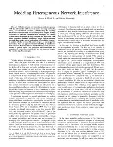
1.2 Overview of The Software Architecture The UML static structure diagram for the DE kernel package is shown in figure 1.4. For model builders, the important class is DEDirector. At the heart of DEDirector is a global event queue that sorts events according to their time stamps, microsteps, and depths (priorities). The DEDirector uses an efficient implementation of the global event queue, a calendar queue data structure [21]. In theory, the time complexity for this particular implementation is O(1) in both enqueue and dequeue operations. This means that the time complexity for enqueue and dequeue operations is independent of the number of pending events in the global event queue. However, to realize this performance, it is necessary for the distribution of events to match certain assumptions. Our calen-


5

DE Domain

DEDirector

Director

+binCountFactor : Parameter(IntToken) +isCQAdaptive : Parameter(BooleanToken) +minBinCount : Parameter(IntToken) +startTime : Parameter(DoubleToken) +stopTime : Parameter(DoubleToken) +stopWhenQueueIsEmpty : Parameter(BooleanToken) +synchronizeToRealTime : Parameter(BooleanToken) #_eventQueue : DEEventQueue #_noMoreActorsToFire : boolean #_stopRequested : boolean -_disabledActors : Set -_microstep : int +DEDirector() +DEDirector(w : Workspace) +DEDirector(c : CompositeEntity, name : String) +fireAtRelativeTime(actor : Actor, time : double) +getEventQueue() : DEEventQueue +getRealStartTimeMillis() : long +getStartTime() : double +getStopTime() : double #_dequeueEvents() : Actor #_disableActor(actor : Actor) #_enqueueEvent(actor : Actor, time : double) #_enqueueEvent(rcv : DEReceiver, tk : Token, time : double) #_enqueueEvent(rcv : DEReceiver, tk : Token) #_getDepth(actor : Actor) : int

AbstractReceiver

1..1

0..n DEReceiver «Interface» Debuggable

-_delay : double -_tokens : LinkedList +DEReceiver() +DEReceiver(container : IOPort) +getDirector() : DEDirector +put(token : Token, time : double) +setDelay(delay : double) #_triggerEvent(token : Token)

«Interface» DEEventQueue

+clear() +get() : DEEvent +isEmpty() : boolean +put(event : DEEvent) +take() : DEEvent

«Interface» Comparable

DEEDirector DECQEventQueue «Interface» CQComparator

-_cQueue : CalendarQueue +DECQEventQueue() +DECQEventQueue(minBinCount : int, binCountFactor : int, isAdaptive : boolean) inner class DEEvent

DECQEventQueue.DECQComparator -_binWidth : DEEvent -_zeroReference : DEEvent +compare(o1 : Object, o2 : Object) : int «Interface» TimedActor

«Interface» SequenceActor

TypedAtomicActor

DEActor

-_actor : Actor -_microstep : int -_receiver : DEReceiver -_receiverDepth : int -_timeStamp : double -_token : Token +DEEvent(rc : DEReceiver, tk : Token, tStamp : double, microstep : int, depth : int) +DEEvent(actor : Actor, timeStamp : double, microstep : int, depth : int) +actor() : Actor +compareTo(event : DEEvent) : final int +depth() : int +isSimultaneousWith(event : DEEvent) : boolean +microstep() : int +receiver() : DEReceiver +timeStamp() : double +token() : Token

+DEActor(container : CompositeEntity, name : String)

TypedIOPort

DEIOPort

+DEIOPort() +DEIOPort(c : ComponentEntity, name : String, isInput : boolean, isOutput : boolean) +DEIOPort(container : ComponentEntity, name : String) +DEIOPort(workspace : Workspace) +broadcast(token : Token, delay : double) +send(channelIndex : int, token : Token, delay : double) : void

FIGURE 1.4. UML static structure diagram for the DE kernel package.

6

Ptolemy II

DE Domain

dar queue implementation observes events as they are dequeued and adapts the structure of the queue according to their statistical properties. Nonetheless, the calendar queue structure will not prove optimal for all models. For extensibility, alternative implementations of the global event queue can be realized by implementing the DEEventQueue interface and specifying the event queue using the appropriate constructor for DEDirector. The DEEvent class carries tokens through the event queue. It contains their time stamp, their microstep, and the depth of the destination actor, as well as a reference to the destination actor. It implements the java.lang.Comparable interface, meaning that any two instances of DEEvent can be compared. The private inner class DECQEventQueue.DECQComparator, which is provided to the calendar queue at the time of its construction, performs the requisite comparisons of events.

1.3 The DE Actor Library The DE domain has a small library of actors in the ptolemy.domains.de.lib package, shown in figure 1.5. The DETransformer base class for actors provides an input and output port. The TimedDelay and Server actors influence the firing priorities as explained below by specifying function dependencies. The Merge actor merges events sequences in chronological order.

1.4 Mutations The DE director tolerates changes to the model during execution. The change should be queued using requestChange(). While invoking those changes, the method invalidateSchedule() is expected to be called, notifying the director that the topology it used to calculate the priorities of the actors is no longer valid. This will result in the priorities being recalculated the next time prefire() is invoked. An example of a mutation is shown in figures 1.6. Figure 1.7 defines a class that constructs a simple model in its constructor. The model consists of a clock connected to a recorder. The method insertClock() creates an anonymous inner class that extends ChangeRequest1. Its execute() method disconnects the two existing actors, creates a new clock and a merge actor, and reconnects the actors as shown in figure 1.6. When the insertClock() method is called, a change request is queued with the top-level composite actor, which delegates the request to the manager. The manager executes the request after the current iteration completes. Thus, the change will always be executed between non-equal time stamps, since an iteration consists of processing all events at the current time stamp. Actors that are added in the change request are automatically initialized. Note, however, one subtlety. The next to last line of the insertClock() method is: _rec.input.createReceivers();

This method call is necessary because the connections of the recorder actor have changed, but since the actor is not new, it will not be reinitialized. Recall that the preinitialize() and initialize() methods are 1. Often a more convenient way to generate mutations is to construct a MoML description of the mutation and issue a MoMLChangeRequest. We are describing here a more direct, low-level mechanism. Note that if you are using actor-oriented classes, you may need to modify this example to propagate the changes from a class definition to instances and/or subclasses, if the changes are made to a class definition. If you use MoML, the propagation is handled for you by the MoML parser.


7

DE Domain

«Interface» Placeable

«Interface» TimedActor

TypedAtomicActor

«Interface» SequenceActor

SingleEvent

Source

Transformer

+trigger : TypedIOPort +output : TypedIOPort

+input : TypedIOPort +output : TypedIOPort

EventButton

Previous

+text : StringAttribute

+initialValue : Parameter

EventFilter

+output : TypedIOPort +time : Parameter(DoubleToken) +value : Parameter

DEActor

DETransformer

WaitingTime

+input : DEIOPort +output : DEIOPort

+output : TypedIOPort(DoubleToken) +waitee : TypedIOPort(Token) +waiter : TypedIOPort(Token) -_waiting : Vector

Queue

Sampler

VariableDelay

+trigger : TypedIOPort(Token) -_queue : FIFOQueue

+trigger : TypedIOPort(Token) -_lastInputs : Token[]

+defaultDelay : Parameter(DoubleToken) +delay : DEIOPort -_delay : double

SamplerWithDefault

TimedDelay

+initialValue : Parameter +trigger : TypedIOPort(Token) -_lastInputs : Token[]

+delay : Parameter(DoubleToken)

Inhibit

QueueWithNextOut

+inhibit : TypedIOPort

+nextOut : TypedIOPort(Token) +trigger : TypedIOPort(Token) -_queue : FIFOQueue

PreemptableTask

Merge

TimeGap

+executionTime : Parameter(DoubleToken) +interrupt : TypedIOPort(Boolean)

Server +newServiceTime : DEIOPort(DoubleToken) +serviceTime : Parameter(DoubleToken) -_nextTimeFree : double

-_previousTime : double

Timer +value : Parameter

FIGURE 1.5. The library of DE-specific actors.

8

Ptolemy II

DE Domain

guaranteed to be called only once, and one of the responsibilities of the preinitialize() method is to create the receivers in all the input ports of an actor. Thus, whenever connections to an input port change during a mutation, the mutation code itself must call createReceivers() to reconstruct the receivers. Note that this will result in the loss of any tokens that might already be queued in the preexisting receivers of the ports. It is because of this possible loss of data that the creation of receivers is not done automatically. The designer of the mutation should be aware of the possible loss of data. There is an additional subtlety about mutations. If an actor locks a resource, such as an I/O port or DatagramSocket, it typically releases this resource in its wrapup() method. However, when the actor is removed while the model is executing, wrapup() never gets called. This case can be handled by overriding the setContainer() method with the following code: public void setContainer(CompositeEntity container) throws IllegalActionException, NameDuplicationException { if (container != getContainer()) { wrapup(); } super.setContainer(container); }

When overriding setContainer() in this way, it is best to make wrapup() idem potent because future implementations of the director might automatically unlock resources of removed actors.

1.5 Writing DE Actors It is very common in DE modeling to include custom-built actors. No pre-defined actor library seems to prove sufficient for all applications. For the most part, writing actors for the DE domain is no different than writing actors for any other domain. Some actors, however, need to exercise particular control over time stamps and actor priorities. The first section below gives general guidelines for writing DE actors and domain-polymorphic actors that work in DE. The second section explains in detail the priorities, and in particular, how to write actors that implement delays. The final section discusses actors that operate as a Java thread.

1.5.1 General Guidelines The points to keep in mind are:

clock merge clock

recorder

recorder clock2 before

after

FIGURE 1.6. Topology before and after mutation for the example in figure 1.7.


9

DE Domain

package ptolemy.domains.de.lib.test; import import import import import import

ptolemy.kernel.util.*; ptolemy.kernel.*; ptolemy.actor.*; ptolemy.actor.lib.*; ptolemy.domains.de.kernel.*; ptolemy.domains.de.lib.*;

public class Mutate { public Manager manager; private private private private

Recorder _rec; Clock _clock; TypedCompositeActor _top; DEDirector _director;

public Mutate() throws IllegalActionException, NameDuplicationException { _top = new TypedCompositeActor(); _top.setName("top"); manager = new Manager(); _director = new DEDirector(); _top.setDirector(_director); _top.setManager(manager); _clock = new Clock(_top, "clock"); _clock.values.setExpression("[1.0]"); _clock.offsets.setExpression("[0.0]"); _clock.period.setExpression("1.0"); _rec = new Recorder(_top, "recorder"); _top.connect(_clock.output, _rec.input); } public void insertClock() { // Create an anonymous inner class ChangeRequest change = new ChangeRequest(_top, "test2") { public void _execute() throws IllegalActionException, NameDuplicationException { _clock.output.unlinkAll(); _rec.input.unlinkAll(); Clock clock2 = new Clock(_top, "clock2"); clock2.values.setExpression("[2.0]"); clock2.offsets.setExpression("[0.5]"); clock2.period.setExpression("2.0"); Merge merge = new Merge(_top, "merge"); _top.connect(_clock.output, merge.input); _top.connect(clock2.output, merge.input); _top.connect(merge.output, _rec.input); // Any pre-existing input port whose connections // are modified needs to have this method called. _rec.input.createReceivers(); _director.invalidateSchedule(); } }; _top.requestChange(change); } }

FIGURE 1.7. An example of a class that constructs a model and then mutates it.

10

Ptolemy II

DE Domain

•

•

• •

•

•

When an actor fires, not all ports have tokens, and some ports may have more than one token. The time stamps of the events that contained these tokens are no longer explicitly available. The current model time (obtained by the getModelTime() method of the director) is assumed to be the time stamp of the events. If the actor leaves unconsumed tokens on its input ports, then it will be iterated again before model time is advanced. This ensures that the current model time is in fact the time stamp of the input events. However, occasionally, an actor will want to leave unconsumed tokens on its input ports, and not be fired again until there is some other new event to be processed. To get this behavior, it should return false from prefire(). This indicates to the DE director that it does not wish to be iterated. If an actor’s output depends on the time stamp of a token with earlier time stamp, it should not leave unconsumed tokens. Instead, it should consume them and store the event and time stamp as a state for future firings. If the actor returns false from postfire(), then the director will not fire that actor again. Events that are destined for that actor are discarded. When an actor produces an output token, the time stamp for the output event is taken to be the current model time. If the actor wishes to produce an event at a future model time, it needs to call the director’s fireAt() method to schedule a future firing, and then to produce the token at that time. If an actor contains a callback method or a private thread and this callback or thread wishes to produce an event now or at a future model time, then a reliable way to achieve this is to call either the fireAtCurrentTime() method or the fireAtRelativeTime() method. These methods may safely be called asynchronously, yielding real-time liveness. By contrast, fireAt() must be called from within the director thread that calls standard actor methods such as prefire(), fire(), and postfire(). By convention in Ptolemy II, actors update their state only in the postfire() method. In DE, the fire() method is only invoked once per iteration, so it may be tempting to ignore this convention and update state in the fire() method. DE actors are often useful in hybrid systems models, where this assumption no longer holds, so we recommend that you only update state in the postfire() method. The simplest way to ensure this is follow the following pattern. For each state variable, such as a private variable named _count, private int _count;

create a shadow variable private int _countShadow;

Then write the methods as follows: public void fire() { _countShadow = _count; ... perform some computation that may modify _countShadow ... } public boolean postfire() { _count = _countShadow; return super.postfire(); }


11

DE Domain

This ensures that the state is updated only in postfire(). In a similar fashion, delayed outputs (produced by either mechanism) should be produced in the postfire() method, since delayed outputs are persistent state. Thus, fireAt() should be called in postfire() only.

1.5.2 Examples TimedDelay Actor. A portion of a domain-specific actor for DE is shown in figure 1.8. This actor delays input events by some amount specified by a parameter. The domain-specific features of the actor are shown in bold. They are: • It overrides the pruneDependencies() method to issue the following statement: removeDependency(input, output);

•

This statement declares to the director that this actor implements a delay from input to output. The director uses this to break the precedences when constructing the DAG to find priorities. In postfire() method, there is an internal calendar queue _delayedOutputTokens to store events that are going to be produced in the future. This actor calls fireAt() method to request future firings to produce those outputs.

Server Actor. The Server actor in the DE library (see figure 1.5) uses a rich set of behavioral properties of the DE domain. A server is a process that takes some amount of time to serve “customers.” While it is serving a customer, other arriving customers have to wait. This actor can have a fixed service time or a variable service time, depending on whether the ParameterPort delay is connected or not. A typical use would be to supply random numbers to the delay port to generate random service times. These times can be provided at the same time as arriving customers to get an effect where each customer experiences a different, randomly selected service time. The (compacted) code is shown in figure 1.9. This actor extends the VariableDelay actor, which extends the TimedDelay actor. The VariableDelay actor overrides the pruneDependencies() method to remove dependencies between the delay port and the output port. package ptolemy.domains.de.lib; public class TimedDelay extends DETransformer { ... ... public boolean postfire() throws IllegalActionException { ... ... if (_currentInput != null) { _delayedOutputTokens.put(new TimedEvent(delayToTime, _currentInput)); getDirector().fireAt(this, delayToTime); } ... ... } public void pruneDependencies() { super.pruneDependencies(); removeDependency(input, output); } ... ... }

FIGURE 1.8. A domain-specific actor, TimedDelay actor, in DE.

12

Ptolemy II

DE Domain

The fire() method first reads and updates the _delay amount. Then it reads the input tokens and store them into the local event queue that stores the delayed input tokens for future processing in the postfire() method. In the end, it checks whether there is some output event scheduled to be produced at the current tag. If there is one, output that event. Otherwise, do nothing. The postfire() method first removes the output token being produced from the local event queue that stores delayed output tokens. If the server is free at the current time, then this actor schedules a future firing to handle the remaining inputs. This is done in the postfire() method rather than the fire() method in keeping with the policy in Ptolemy II that persistent state is not updated in the fire() method. Note that if an actor does not consume input tokens that are available in the fire() method, it is essential that prefire() returns false. Otherwise, the DE scheduler will keep firing the actor until the inputs are all consumed, which will never happen if the actor is not consuming inputs! package ptolemy.domains.de.lib; public class Server extends VariableDelay { public PortParameter delay; public void fire() throws IllegalActionException { delay.update(); _delay = ((DoubleToken) delay.getToken()).doubleValue(); Time currentTime = getDirector().getModelTime(); if (input.hasToken(0)) { _currentInput = input.get(0); _delayedInputTokensList.addLast(_currentInput); } else { _currentInput = null; } _currentOutput = null; if (_delayedOutputTokens.size() > 0) { if (currentTime.compareTo(_nextTimeFree) == 0) { TimedEvent earliestEvent = (TimedEvent) _delayedOutputTokens.get(); Time eventTime = earliestEvent.timeStamp; if (!eventTime.equals(currentTime)) { throw new InternalErrorException("Service time is " + "reached, but output is not available."); } _currentOutput = (Token) earliestEvent.contents; output.send(0, _currentOutput); } } } public void initialize() throws IllegalActionException { super.initialize(); _nextTimeFree = Time.NEGATIVE_INFINITY; _delayedInputTokensList = new LinkedList(); } public boolean postfire() throws IllegalActionException { Time currentTime = getDirector().getModelTime(); if (_currentOutput != null) { _delayedOutputTokens.take(); } if ((_delayedInputTokensList.size() != 0) && _delayedOutputTokens.isEmpty()) { _nextTimeFree = currentTime.add(_delay); _delayedOutputTokens.put(new TimedEvent(_nextTimeFree, _delayedInputTokensList.removeFirst())); getDirector().fireAt(this, _nextTimeFree); } return !_stopRequested; } }

FIGURE 1.9. Code for the Server actor. For more details, see the source code.


13

DE Domain

1.5.3 Thread Actors1 In some cases, it is useful to describe an actor as a thread that waits for input tokens on its input ports. The thread suspends while waiting for input tokens and is resumed when some or all of its input ports have input tokens. While this description is functionally equivalent to the standard description explained above, it leverages on the Java multi-threading infrastructure to save the state information. Consider the code for the ABRecognizer actor shown in figure 1.10. The two code listings implement two actors with equivalent behavior. The left one implements it as a threaded actor, while the right one implements it as a standard actor. We will from now on refer to the left one as the threaded description and the right one as the standard description. In both descriptions, the actor has two input ports, inportA and inportB, and one output port, outport. The behavior is as follows. Produce an output event at outport as soon as events at inportA and inportB occurs in that particular order, and repeat this behavior. Note that the standard description needs a state variable state, unlike the case in the threaded description. In general the threaded description encodes the state information in the position of the code, while the standard description encodes it explicitly using state variables. While it is true that the context switching overhead associated with multi-threading application reduces the performance, we argue that the simplicity and clarity of writing actors in the threaded fashion is well worth the cost in some applications. To write an actor in the threaded fashion, one simply derives from the DEThreadActor class and implements the run() method. In many cases, the content of the run() method is enclosed in the infinite ‘while(true)’ loop since many useful threaded actors do not terminate. The waitForNewInputs() method is overloaded and has two flavors, one that takes no arguments public class ABRecognizer extends DEThreadActor { StringToken msg = new StringToken("Seen AB");

public class ABRecognizer extends DEActor { StringToken msg = new StringToken("Seen AB");

// the run method is invoked when the thread // is started. public void run() { while (true) { waitForNewInputs(); if (inportA.hasToken(0)) { IOPort[] nextInport = {inportB}; waitForNewInputs(nextInport); outport.broadcast(msg); } } }

// We need an explicit state variable in // this case. int state = 0; public void fire() { switch (state) { case 0: if (inportA.hasToken(0)) { state = 1; break; } case 1: if (inportB.hasToken(0)) { state = 0; outport.broadcast(msg); } } } }

FIGURE 1.10. Code listings for two style of writing the ABRecognizer actor.

1. This section describes techniques that have not been widely used, and are not extensively tested.

14

Ptolemy II

DE Domain

and another that takes an IOPort array as argument. The first suspends the thread until there is at least one input token in at least one of the input ports, while the second suspends until there is at least one input token in any one of the specified input ports, ignoring all other tokens. In the current implementation, both versions of waitForNewInputs() clear all input ports before the thread suspends. This guarantees that when the thread resumes, all tokens available are new, in the sense that they were not available before the waitForNewInput() method call. The implementation also guarantees that between calls to the waitForNewInputs() method, the rest of the DE model is suspended. This is equivalent to saying that the section of code between calls to the waitForNewInput() method is a critical section. One immediate implication is that the result of the method calls that check the configuration of the model (e.g. hasToken() to check the receiver) will not be invalidated during execution in the critical section. It also means that this should not be viewed as a way to get parallel execution in DE. For that, consider the DDE domain. It is important to note that the implementation serializes the execution of threads, meaning that at any given time there is only one thread running. When a threaded actor is running (i.e. executing inside its run() method), all other threaded actors and the director are suspended. It will keep running until a waitForNewInputs() statement is reached, where the flow of execution will be transferred back to the director. Note that the director thread executes all non-threaded actors. This serialization is needed because the DE domain has a notion of global time, which makes parallelism much more difficult to achieve. The serialization is accomplished by the use of monitor in the DEThreadActor class. Basically, the fire() method of the DEThreadActor class suspends the calling thread (i.e. the director thread) until the threaded actor suspends itself (by calling waitForNewInputs()). One key point of this implementation is that the threaded actors appear just like an ordinary DE actor to the DE director. The DEThreadActor base class encapsulates the threaded execution and provides the regular interfaces to the DE director. Therefore the threaded description can be used whenever an ordinary actor can, which is everywhere. The code shown in figure 1.11 implements the run method of a slightly more elaborate actor with the following behavior: Emit an output O as soon as two inputs A and B have occurred. Reset this behavior each time the input R occurs. Recent work has extended the DE Director to support parallel execution in the form of actors containing private threads and callbacks. Future work in this area may involve extending the infrastructure to support additional concurrency constructs, such as preemption, other forms of parallel execution, etc. It might also be interesting to explore new concurrency semantics similar to the threaded DE, but without the ‘forced’ serialization.

1.6 Composing DE with Other Domains One of the major concepts in Ptolemy II is modeling heterogeneous systems through the use of hierarchical heterogeneity. Actors on the same level of hierarchy obey the same set of semantics rules. Inside some of these actors may be another domain with a different model of computation. This mechanism is supported through the use of opaque composite actors. An example is shown in figure 1.12. The outermost domain is DE and it contains seven actors, two of them are opaque and composite. The opaque composite actors contain subsystems, which in this case are in the DE and CT domains.


15

DE Domain

1.6.1 DE inside Another Domain The DE subsystem completes one iteration whenever the opaque composite actor is fired by the outer domain. One of the complications in mixing domains is in the synchronization of time. Denote the current time of the DE subsystem by tinner and the current time of the outer domain by touter. An iteration of the DE subsystem is similar to an iteration of a top-level DE model, except that prior to the iteration tokens are transferred from the ports of the opaque composite actors into the ports of the contained DE subsystem, and after the end of the iteration, the director requests a refire at the smallest time stamp in the event queue of the DE subsystem. This presumes that the DE subsystem knows at what time stamp the it, or one of its contained actors, will wish to be refired. Future work may remove this limitation, allowing real-time events (such as from I/O) to propagate out of a DE subsystem. Currently the DE domain can handle such asynchronous events only if it is not inside another domain. public void run() { try { while (true) { // In initial state.. waitForNewInputs(); if (R.hasToken(0)) { // Resetting.. continue; } if (A.hasToken(0)) { // Seen A.. IOPort[] ports = {B,R}; waitForNewInputs(ports); if (!R.hasToken(0)) { // Seen A then B.. O.broadcast(new DoubleToken(1.0)); IOPort[] ports2 = {R}; waitForNewInputs(ports2); } else { // Resetting continue; } } else if (B.hasToken(0)) { // Seen B.. IOPort[] ports = {A,R}; waitForNewInputs(ports); if (!R.hasToken(0)) { // Seen B then A.. O.broadcast(new DoubleToken(1.0)); IOPort[] ports2 = {R}; waitForNewInputs(ports2); } else { // Resetting continue; } } // while (true) } catch (IllegalActionException e) { getManager().notifyListenersOfException(e); } }

FIGURE 1.11. The run() method of the ABRO actor.

16

Ptolemy II

DE Domain

The transfer of tokens from the ports of the opaque composite actor into the ports of the contained DE subsystem actors is done in the transferInputs() method of the DE director. This method is extended from its default implementation in the Director class. The implementation in the DEDirector class advances the current time of the DE subsystem to the current time of the outer domain, then calls super.transferInputs(). It is done in order to correctly associate tokens seen at the input ports of the opaque composite actor, if any, with events at the current time of the outer domain, touter, and put these events into the global event queue. This mechanism is, in fact, how the DE subsystem synchronize its current time, tinner, with the current time of the outer domain, touter.(Recall that the DE director advances time by looking at the smallest time stamp in the event queue of the DE subsystem). Specifically, before the advancement of the current time of the DE subsystem tinner is less than or equal to the touter, and after the advancement tinner is equal to the touter. Requesting a refiring is done in the postfire() method of the (inner) DE director by calling the fireAt() method of the executive (outer) director. Its purpose is to ensure that events in the DE subsystem are processed on time with respect to the current time of the outer domain, touter. Note that if the DE subsystem is fired due to the outer domain processing a refire request, then there may not be any tokens in the input port of the opaque composite actor at the beginning of the DE subsystem iteration. In that case, no new events with time stamps equal to touter will be put into the global event queue. Interestingly, in this case, the time synchronization will still work because tinner will be advanced to the smallest time stamp in the global event queue which, in turn, has to equal touter because we always request a refire according to that time stamp.

Discrete Event

Discrete Event

Interruptible Server

DEPoisson

Sin

+

1/s

Process Delay

1/s

K(z)

ZOH

Continuous Time

FIGURE 1.12. An example of heterogeneous and hierarchical composition. The CT subsystem and DE subsystem are inside an outermost DE system. This example is developed by Jie Liu [100].


17

DE Domain

1.6.2 Another Domain inside DE Due to its nature, any opaque composite actor inside DE is opaque and therefore, as far as the DE Director is concerned, behaves exactly like a domain polymorphic actor. Recall that domain polymorphic actors are treated as functions with zero delay in computation time. To produce events in the future, domain polymorphic actors request a refire from the DE director and then produce the events when it is refired.

18

Ptolemy II

CT Domain Author:

Jie Liu Haiyang Zheng

2.1 Introduction The continuous-time (CT) domain in Ptolemy II aims to help the design and simulation of systems that can be modeled using ordinary differential equations (ODEs). ODEs are often used to model analog circuits, plant dynamics in control systems, lumped-parameter mechanical systems, lumpedparameter heat flows and many other physical systems. Let’s start with an example. Consider a second order differential system, mz··( t ) + bz· ( t ) + kz ( t ) = u ( t ) y(t) = c ⋅ z(t ) z ( 0 ) = 10, z· ( 0 ) = 0.

(1)

The equations could be a model for an analog circuit as shown in figure 2.1(a), where z is the voltage u proof-mass

1

R1

2

R2

3

I1 u

+

+ -

C1

C2

z

m

z

R3 + R4

-

Fk

y

k

b

Fb

Substrate

(a) A circuit implementation.

(b) A mechanical implementation.

FIGURE 2.1. Possible implementations of the system equations.


19

CT Domain

of node 3, and m = R1 ⋅ R2 ⋅ C1 ⋅ C2 k = R1 ⋅ C1 + R2 ⋅ C2 b = 1 c = R4 ⁄ ( R3 + R4 ) .

(2)

Or it could be a lumped-parameter spring-mass mechanical model for the system shown in figure 2.1(b), where z is the position of the mass, m is the mass, k is the spring constant, b is the damping parameter, and c = 1. In general, an ODE-based continuous-time system has the following form: (3) x· = f ( x, u, t ) y = g ( x , u, t ) x ( t0 ) = x0 ,

(4) (5) n

where, t ∈ ℜ , t ≥ t 0 , a real number, is continuous time. At any time t, x ∈ ℜ , an n-tuple of real numm l bers, is the state of the system; u ∈ ℜ is the m-dimensional input of the system; y ∈ ℜ is the ln dimensional output of the system; x· ∈ ℜ is the derivative of x with respect to time t , i.e. ------ . x· = dx dt

(6)

Equations (3), (4), and (5) are called the system dynamics, the output map, and the initial condition of the system, respectively. For example, for the mechanical system above, if we define a vector x(t) = z(t ) , z· ( t )

(7)

then system (1) can be written in form of (3)-(5), like 1 x· ( t ) = ---- 0 1 x ( t ) + 0 u ( t ) m –k –b 1⁄m

(8)

y(t) = c 0 x(t) x ( 0 ) = 10 . 0 The solution, x(t), of the set of ODE (3)-(5), is a continuous function of time, also called a waveform, which satisfies the equation (3) and initial condition (5). The output of the system is then defined as a function of x(t) and u(t), which satisfies (4). The precise solution of a set of ODEs is usually impossible to be found using digital computers. Numerical solutions are approximations of the precise solution. A numerical solution of ODEs are usually done by integrating the right-hand side of (3) on a discrete set of time points. Using digital computers to simulate continuous-time systems has been studied for more than three decades. One of the most well-known tools is Spice [112]. The CT domain differs from Spice-like continuous-time simulators in two ways — the system specification is somewhat different, and it is designed to interact with other models of computation.

20

Ptolemy II

CT Domain

2.1.1 System Specification There are usually two ways to specify a continuous-time system, the conservation-law model and the signal-flow model [63]. The conservation-law models, like the nodal analysis in circuit simulation [60] and bond graphs [128] in mechanical models, define systems by their physical components, which specify relations of cross and through variables, and conservation laws are used to compile the component relations into global system equations. For example, in circuit simulation, the cross variables are voltages, the through variables are currents, and the conservation laws are Kirchhoff’s laws. This model directly reflects the physical components of a system, thus is easy to construct from a potential implementation. The actual mathematical representation of the system is hidden. In signal-flow models, entities in a system are maps that define the mathematical relation between their input and output signals. Entities communicate by passing signals. This kind of models directly reflects the mathematical relations among signals, and is more convenient for specifying systems that do not have an explicit physical implementation yet. In the CT domain of Ptolemy II, the signal-flow model is chosen as the interaction semantics. The conservation-law semantics may be used within an entity to define its I/O relation. There are four major reasons for this decision: 1. The signal-flow model is more abstract. Ptolemy II focuses on system-level design and behavior simulation. It is usually the case that, at this stage of a design, users are working with abstract mathematical models of a system, and the implementation details are unknown or not cared about. 2. The signal flow model is more flexible and extensible, in the sense that it is easy to embed components that are designed using other models. For example, a discrete controller can be modeled as a component that internally follows a discrete event model of computation but exposes a continuous-time interface. 3. The signal flow model is consistent with other models of computation in Ptolemy II. Most models of computation in Ptolemy use message-passing as the interaction semantics. Choosing the signalflow model for CT makes it consistent with other domains, so the interaction of heterogeneous systems is easy to study and implement. This also allows domain polymorphic actors to be used in the CT domain. 4. The signal flow model is compatible with the conservation law model. For physical systems that are based on conservation laws, it is usually possible to wrap them into an entity in the signal flow model. The inputs of the entity are the excitations, like the current on ideal current sources, and the outputs are the variables that the rest of the system may be interested in. The signal flow block diagram of the system (3) - (5) is shown in figure 2.2. The system dynamics (3) is built using integrators with feedback. In this figure, u, x· , x, and y, are continuous signals flowing from one block to the next. Notice that this diagram is only conceptual, most models may involve mul-

u f( )

. x

x

g( )

y

FIGURE 2.2. A conceptual block diagram for continuous time systems.


21

CT Domain

tiple integrators1. Time is shared by all components, so it is not considered as an input. At any fixed time t, if the “snapshot” values x(t) and u(t) are given, then x· ( t ) and y(t) can be found by evaluating f and g, which can be achieved by firing the respective blocks. The “snapshot” of all the signals at t is called the behavior of the system at time t . The signal-flow model for the example system (1) is shown in figure 2.3. For comparison purpose, the conservation-law model (modified nodal analysis) of the system shown in figure 2.1(a) is shown in (9). 1 ------R1

1– -----0 0 R1 d 1- -----1- + -----1- + C1 ---1– -----– -----0 dt R1 R1 R2 R2 d 11- + -----1- + C2 ---1- – -----0 – ----------dt R2 R2 R3 R3 11- + -----10 0 – ----------R3 R3 R4 1

0

0

0

–1 0

v1 v2

0

v3

0

y I1

0 0 = 0 0 u

(9)

0

By doing some math, we can see that (9) and (8) are in fact equivalent. Equation (9) can be easily assembled from the circuit, but it is more complicated than (8). Notice that in (9) d/dt is the derivative operator, which is replaced by an integration algorithm at each time step, and the system equations reduce to a set of algebraic equations. Spice software is known to have a very good simulation engine for models in form of (9).

2.1.2 Time One distinct characterization of the CT model is the continuity of time. This implies that a continuous-time system have a behavior at any time instance. The simulation engine of the CT model should be able to compute the behavior of the system at any time point, although it may march discretely in time. In order to achieve an accurate simulation, time should be carefully discretized. The discretization of time, which appears as integration step sizes, may be determined by time points of interest (e.g. U

u

G1 1/m

A

S1

S2

+

G4

Y

C

y

G2 -b/m

G3 -k/m

FIGURE 2.3. The block diagram for the example system.

1. Ptolemy II does not support vectorization in the CT domain yet.

22

Ptolemy II

CT Domain

discontinuities), by the numerical error of integration, and by the convergence in solving algebraic equations. Time is also global, which means that all components in the system share the same notion of time.

2.2 Solving ODEs numerically We outline some basic terminologies on numerical ODE solving techniques that are used in this chapter. This is not a summary of numerical ODE solving theory. For a detailed treatment for ODEs and their numerical solutions, please refer to books on numerical solutions for ODEs, e.g. [45]. Not all ODEs have a solution, and some ODEs have more than one solution. In such situations, we say that the solution is not well defined. This is usually a result of errors in the system modeling. We restrict our discussion to systems that have unique solutions. Theorem 1 in Appendix A states the conditions for the existence and uniqueness of solutions of ODEs. Roughly speaking, we denote by D a set in ℜ which contains at most a finite number of points per unit interval, and let u be piecewise-continuous on ℜ – D . Then, for any fixed u(t), if f is also piecewise-continuous on ℜ – D , and f satisfies the Lipschitz condition (see e.g. [45]), then the ODE (3) with the initial condition (5) has a unique solution. The solution is called the state trajectory of the system. The key of simulating a continuous-time system numerically is to find an accurate numerical approximation of the state trajectory.

2.2.1 Basic Notations Usually, only the solution on a finite time interval [t 0,t f] is needed. A simulation of the system is performed on discrete time points in this interval. We denote by Tc = { t 0, t 1, t 2, …t n, …t f }, Tc ⊂ [ t 0, t f ] ,

(10)

t0 < t1 < t2 < … < tn < … < tf ,

(11)

where

the set of the discrete time points of interest. To explicitly illustrate the discretization of time and the difference between the precise solution and the numerical solution, we use the following notation in the rest of the chapter: • t n : the n-th time point, to explicitly show the discretization of time. However, we write t, if the index n is not important. • x [ t i, t j ] : the precise (continuous) state trajectory from time t i to t j ; • x ( tn ) : the precise solution of (3) at time t n ; •

x t : the numerical solution of (3) at time t n ;

•

h n = t n – t n – 1 : step size of numerical integration. We also write h if the index n in the sequence

n

is not important. For accuracy reason, h may not be uniform. •

x ( t n ) – x tn : the 2-normed difference between the precise solution and the numerical solution at step n is called the (global) error at step n; the difference, when we assume x t …x t 0

n–1

are precise,

is called the local error at step n. Local errors are usually easy to estimate and the estimation can be used for controlling the accuracy of numerical solutions.


23

CT Domain

A general way of numerically simulating a continuous-time system is to compute the state and the output of the system in an increasing order of t n . Such algorithms are called the time-marching algorithms, and, in this chapter, we only consider these algorithms. There are variety of time marching algorithms that differ on how x t is computed given x t …x t . The choice of algorithms is applican 0 n–1 tion dependent, and usually reflects the speed, accuracy, and numerical stability trade-offs.

2.2.2 Fixed-Point Behavior Numerical ODE solving algorithms approximate the derivative operator in (3) using the history and the current knowledge on the state trajectory. That is, at time t n , the derivative of x is approximated by a function of x t , …, x t , x t , i.e. 0

n–1

n

x· t = p ( x t , …, x t n

0

n–1

, xt ) . n

(12)

Plugging (3) in this, we get p ( x t …x t 0

, x t ) = f ( x t , u ( t n ), t n )

n–1

n

n

(13)

Depending on whether x tn explicitly appears in (13), the algorithms are called explicit integration algorithms or implicit integration algorithms. That is, we end up solving a set of algebraic equations in one of the two forms: x tn = F E ( x t0, …, x t

)

(14)

n–1

or F I ( x t , …, x t ) = 0 , 0

(15)

n

where F E and F I are derived from the time t n , the input u ( t n ) , the function f, and the history of x and x· . Solving (14) or (15) at a particular time t n is called an iteration of the CT simulation at t n . Equation (14) can be solved simply by a function evaluation and an assignment. But the solution of (15) is the fixed point of FI, which may not exist, may not be unique, or may not be able to be found. The contraction mapping theorem [21] shows the existence and uniqueness of the fixed-point solution, and provides one way to find it. Given the map FI that is a local contraction map (generally true for small enough step sizes) and let an initial guess σ 0 be in the contraction radius, then a unique fixed point exists and can be found by iteratively computing: σ 1 = F E ( σ 0 ), σ 2 = F E ( σ 1 ), σ 3 = F E ( σ 2 ), …

(16)

Solving both (14) and (15) should be thought of as finding the fixed-point behavior of the system at a particular time. This means both functions F E and F I should be smooth w.r.t. time, during one iteration of the simulation. This further implies that the topology of the system, all the parameters, and all the internal states that the firing functions depend on should be kept unchanged. We require that domain polymorphic actors to update internal states only in the postfire() method exactly for this reason.

2.2.3 ODE Solvers Implemented The following solvers has been implemented in the CT domain.

24

Ptolemy II

CT Domain

1. Forward Euler solver: x tn + 1 = x tn + h n + 1 ⋅ x· tn = x tn + h n + 1 ⋅ f ( x t n, u tn, t n )

(17)

2. 2(3)-order Explicit Runge-Kutta solver K 0 = h n + 1 ⋅ f ( x tn, u tn, t n )

(18)

K 1 = h n + 1 ⋅ f ( x t + K 0 ⁄ 2, u t n

n

+ h n + 1 ⁄ 2, t n

K 2 = h n + 1 ⋅ f ( x t + 3K 1 ⁄ 4, u t n

x˜ t

n

+ hn + 1 ⁄ 2 )

+ 3h n + 1 ⁄ 4, t n

+ 3h n + 1 ⁄ 4 )

2 1 4 = x t + --- K 0 + --- K 1 + --- K 2 n 9 3 9

n+1

with error control: K 3 = h n + 1 ⋅ f ( x˜ tn + 1, u tn + 1, t n + 1 )

(19)

1 1 1 5 LTE = – ------ K 0 + ------ K 1 + --- K 2 – --- K 3 12 9 8 72 if LTE < ErrorTolerance , x t = x˜ t , otherwise, fail. If this step is successful, the next n+1 n+1 integration step size is predicted by: h n + 2 = h n + 1 ⋅ max ( 0.5, 0.8 ⋅ 3 ( ErrorTolerance ) ⁄ LTE )

(20)

3. 4(5)-order Explicit Runge-Kutta solver1 K0 = hn + 1 ⋅ f ( xt , ut , tn ) n

K 1 = h n + 1 ⋅ f ( x t + K 0 ⁄ 5, u t n

(21)

n

n

+ h n + 1 ⁄ 5, t n

+ hn + 1 ⁄ 5 )

K 2 = h n + 1 ⋅ f ( x t + 3K 0 ⁄ 40 + 9K 1 ⁄ 40, u t n

n

+ 3h n + 1 ⁄ 10, t n

K 3 = h n + 1 ⋅ f ( x t + 3K 0 ⁄ 10 – 9K 1 ⁄ 10 + 6K 2 ⁄ 5, u t n

n

+ 3h n + 1 ⁄ 10 )

+ 3h n + 1 ⁄ 5, t n

+ 3h n + 1 ⁄ 5 )

K 4 = h n + 1 ⋅ f ( x t – 11K 0 ⁄ 54 + 5K 1 ⁄ 2 – 70K 2 ⁄ 27 + 35K 3 ⁄ 27, u t n

n

+ h n + 1, t n

+ hn + 1 )

K 5 = h n + 1 ⋅ f ( x tn + 1631K 0 ⁄ 55296 + 175K 1 ⁄ 512 + 575K 2 ⁄ 13824 + 44275K 3 ⁄ 110592 + 253K 4 ⁄ 4096, u t n + 7h n + 1 ⁄ 8, t n + 7h n + 1 ⁄ 8 ) 37 250 125 512 x˜ tn + 1 = x tn + --------- K 0 + --------- K 1 + --------- K 2 + ------------ K 5 378 621 594 1771

1. This algorithm is based on "A Variable Order Runge-Kutta Method for Initial Value Problems with Rapidly Varying Right-Hand Sides" by J. R. Cash and A. H. Karp, ACM Transactions on Mathematical Software, 16(3), 201-222 (1990).


25

CT Domain

with error control: K 6 = h n + 1 ⋅ f ( x˜ t

n+1

, ut

, tn + 1 )

(22)

n+1

277 37- – -------------2825-⎞ K + ⎛ 250 --------- – 18575 ---------------⎞ K + ⎛ 125 --------- – 13525 ---------------⎞ K – --------------- K LTE = ⎛ -------⎝ 378 27648⎠ 0 ⎝ 621 48384⎠ 2 ⎝ 594 55296⎠ 3 14336 4 512 1 + ⎛ ------------ – ---⎞ K 5 ⎝ 1771 4⎠ = x˜ t , otherwise, fail. If this step is successful, the next if LTE < ErrorTolerance , x t n+1 n+1 integration step size is predicted by: h n + 2 = h n + 1 ⋅ 5 ( ErrorTolerance ) ⁄ LTE

(23)

4. Backward Euler solver: x tn + 1 = x tn + h n + 1 ⋅ x· tn + 1 = xt + hn + 1 ⋅ f ( xt , ut n

n+1

(24) , tn + 1 )

n+1

5. Trapezoidal Rule solver: hn + 1 x tn + 1 = x tn + ------------ ( x· tn + x· tn + 1 ) 2 hn + 1 = x t + ------------ ( x· t + f ( x t , u t , t n + 1 ) ) n n n+1 n+1 2

.

(25)

Among these solvers, 1), 2) and 3) are explicit; 4) and 5) are implicit. Also, 1) and 4) do not perform step size control, so are called fixed-step-size solvers; 2), 3), and 5) change step sizes according to error estimation, so are called variable-step-size solvers. Variable-step-size solvers adapt the step sizes according to changes of the system flow, thus are “smarter” than fixed-step-size solvers.

2.2.4 Discontinuity The existence and uniqueness of the solution of an ODE (Theorem 1 in Appendix A) allows the right-hand side of (3) to be discontinuous at a discrete set D1, and the elements in this discrete set are called the breakpoints (also called the discontinuous points in some literature). These breakpoints may be caused by the discontinuity of input signal u, or by the intrinsic flow of f. At these points, the solutions are defined based on a discrete-event semantics and achieved by performing discrete phase of executions. Discrete phase of executions solve the final values at breakpoints, which are the solutions defined on the right limits. The left limits of the solutions, which are called initial values at breakpoints, are solved with the normal continuous-time equations based on the ODE. One impact of breakpoints on ODE solvers is that history solutions are useless when approximating the derivative of x after the breakpoints. The solver should resolve the new initial conditions and start the solving process as if it is at a starting point. So, the discretization of time should step exactly on breakpoints for the left limit, and start at the breakpoint again after finding the right limit. A breakpoint may be known beforehand, in which case it is called a predictable breakpoint. For 1. A discrete set is an ordered set for which there exists an order embedding to the natural numbers.

26

Ptolemy II

CT Domain

example, a square wave source actor knows its next flip time. This information can be used to control the discretization of time. A breakpoint can also be unpredictable, which means it is unknown until the time it occurs is passed. For example, an actor that varies its functionality when the input signal crosses a threshold can only report a “missed” breakpoint after an integration step is finished. How to handle breakpoints correctly is a big challenge for integrating continuous-time models with discrete models like DE and FSM.

2.2.5 Breakpoint ODE Solvers Breakpoints in the CT domain are handled by adjusting integration steps. We use a table to handle predictable breakpoints, and use the step size control mechanism to handle unpredictable breakpoints. The breakpoint handling are transparent to users, and the implementation details (provided in section 2.8.4) are only needed when developing new directors, solvers, or event generators. Since the history information is useless at breakpoints, a special ODE solver is designed to restart the numerical integration process. In particular, we have implemented the DerivativeResolver, which calculates the derivative of the current state, i.e. ( dx ) ⁄ ( dt ) . This is simply done by evaluation the right-hand side of (3). At breakpoints, this solver is used for the first step to generate history information for explicit methods or one step methods. Notice that this solver does not advance time and it can only be used at breakpoints.

2.3 Signal Types The CT domain of Ptolemy II supports continuous time mixed-signal modeling. As a consequence, there could be two types of signals in a CT model: continuous signals and discrete events. Note that for both types of signals, time is continuous. These two types of signals directly affect the behavior of a receiver that contains them. A continuous CTReceiver contains a sample of a continuous signal at the current time. Reading a token from that receiver will not consume the token. A discrete CTReceiver may or may not contain a discrete event. Reading from a discrete CTReceiver with an event will consume the event, so that events are processed exactly once1. Reading from an empty discrete CTReceiver is not allowed. Note that some actors can be used to compute on both continuous and discrete signals. For example, an adder can add two continuous signals, as well as two sets of discrete events. Whether a particular link among actors is continuous or discrete is resolved by a signal type system. The signal type system understands signal types on specific actors (indicated by the interfaces they implement or the parameters specified on their ports), and try to resolve signal types on the ports of domain polymorphic actors. The signal type system in the CT domain works on a simple lattice of signal types, shown in Figure 2.4. A type lower in the lattice is more specific than a type higher in the lattice. A CT model is well-defined and executable, if and only if all ports are resolved to either CONTINUOUS or DISCRETE. Some actors have their signal types fixed. For example, an Integrator has a CONTINUOUS input and a CONTINUOUS output; a PeriodicSampler has a CONTINUOUS input and a DISCRETE output; a TriggeredSampler has one CONTINUOUS input (the input), one DISCRETE input (the trigger), and a DISCRETE output; and a ZeroOrderHold has a DISCRETE input and a CONTINUOUS output. For domain polymorphic actors that implement the SequenceActor 1. This distinction of receivers is also called state and event semantics in some literatures [70].


27

CT Domain

interface, i.e. they operate solely on sequences of tokens, their inputs and outputs are treated as DISCRETE. For other domain polymorphic actors that can operate on both continuous and discrete signals, the signal type on their ports are initially UNRESOLVED. The signal type system will resolve and check signal types of ports according to the following two rules: • If a port p is connected to another port q with a more specific type, then the type of p is resolved to that of the port q. If p is CONTINUOUS but q is DISCRETE, then both of them are resolved to NOT-A-TYPE. • Unless otherwise specified, the types of the input ports and output ports of an actor are the same. At the end of the signal-type resolution, if any port is of type UNRESOLVED or NOT-A-TYPE, then the topology of the system is illegal, and the execution is denied. The signal type of a port can also be forced by adding an parameter “signalType” to the port. The signal type system will recognize this parameter and resolve other types accordingly. To add this parameter, right click on the port, select Configure, then add a parameter with the name signalType and the value of a string of either “CONTINUOUS” or “DISCRETE”, noting the quotation marks. Signal types may be more trickier at the boundaries of opaque composite actors than within a CT model. Because of the information hiding, it may not be obvious which port of another level of hierarchy is continuous and which port is discrete. In the CT domain, we follow these rules to resolve signal types for composite ports: • A TypedCompositeActor within a CT model is always treated as entirely discrete. Within a CT model, for any opaque composite actor that may contain continuous dynamics at a deeper level, use the CTCompositeActor (listed in the actor library as “continuous time composite actor” in domain specific actors) or the modal model composite actor. • For a CTCompositeActor or a modal model within a CT model, all its ports are treated as continuous by default. To allow a discrete event going through the composite actor boundary, manually set the signal type of that port by adding the signalType parameter. • For a TypedCompositeActor containing a CT model, all the ports of the TypedCompositeActor are treated as discrete, and the CT director to use is the CTMixedSignalDirector (listed as CTDirector in the vergil director library). • For a CTCompositeActor or a modal model containing a CT model, all the signal types of the ports of the container are treated as continuous, and can be set by adding the signalType parameter. The CTDirector to use in this situation is the CTEmbeddedDirector.

UNRESOLVED

CONTINUOUS

DISCRETE

NOT-A-TYPE FIGURE 2.4. A signal type lattice.

28

Ptolemy II

CT Domain

2.4 CT Actors A CT system can be built up using actors in the ptolemy.domains.ct.lib package and domain polymorphic actors that have continuous behaviors (i.e. all actors that do not implement the SequenceActor interface). The key actor in CT is the integrator. It serves the unique role of wiring up ODEs. Other actors in a CT system are usually stateless. A general understanding is that, in a pure continuous-time model, all the information — the state of the system— is stored in the integrators.

2.4.1 CT Actor Interfaces In order to schedule the execution of actors in a CT model and to support the interaction between CT and other domains (which are usually discrete), we provide the following interfaces. • CTDynamicActor. Dynamic actors are actors that contains continuous dynamics in their I/O path. An integrator is a dynamic actor, and so are all actors that have integration relations from their inputs to their outputs. • CTEventGenerator. Event generators are actors that convert continuous time input signals to discrete output signals. • CTStatefulActor. Stateful actors are actors that have internal states. The reason to classify this kind of actor is to support rollback, which may happen when a CT model is embedded in a discrete event model. • CTStepSizeControlActor. Step size control actors influence the integration step size by telling the director whether the current step is accurate. The accuracy is in the sense of both tolerable numerical errors and absence of unpredictable breakpoints. It may also provide information about refining a step size for an inaccurate step and suggesting the next step size for an accurate step. • CTWaveformGenerator. Waveform generators are actors that convert discrete input signals to continuous-time output signals. Strictly speaking, event generators and waveform generators do not belong to any domain, but the CT domain is design to handle them intrinsically. When building systems, CT parts always provide discrete interface to other domains. A loop containing only dynamic actors or a loop containing only non-dynamic actors are not allowed in a CT model. They introduce problems about the order that actors are executed. A loop only containing dynamic actors can be easily broken by a Scale actor with scale 1. A loop of non-dynamic actors builds an algebraic equation. The CT domain does not support modeling algebraic equations, yet.

2.4.2 Actor Library ContinuousClock. This clock actor generates a periodic continuous-time signal with regularly spaced intervals. The time interval is specified by the period and offset parameters, where the offset parameter contains an array of strictly increasing values that do not exceed the period value. The values of the signal are specified by the values parameter. The values parameter also contains an array and the length of this array should be the same as the array length of the offset parameter. This clock actor is different from the normal clock actor (called DiscreteClock) in the actor.lib directory in two ways. First, this actor has a value at any time point. Second, at each offset, this actor produces two values, where the first one is the left limit and second value is the right limit.


29

CT Domain

ContinuousTransferFunction. A transfer function in the continuous time domain. This actor implements a transfer function where the single input (u) and single output (y) can be expressed in (Laplace) transfer function form as the following equation: m–1

m–2

+ b2 s + … + bm Y ( s ) = b-----------------------------------------------------------------1s ----------n–1 n–2 U(s) a1 s + a2 s + … + an

(26)

where m and n are the number of numerator and denominator coefficients, respectively. This actors has two parameters − numerator and denominator − containing the coefficients of the numerator and denominator in descending powers of s. The parameters are double arrays. The order of the denominator (n) must be greater than or equal to the order of the numerator (m). CTPeriodicalSampler. This event generator periodically samples the input signal and generates events with the value of the input signal at these time points. The values are always the initial values of the input signal. The sampling rate is given by the samplePeriod parameter, which has default value 0.1. The sampling time points, which are known beforehand, are examples of predictable breakpoints. CTRateLimiter. This actor limits the first derivative of the input signal so that the output signal does not change faster than the specified limit. CTTriggeredSampler. This actor samples the continuous input signal when there is a discrete event present at the trigger input. Note that this sampler can generate values other than initial values of the input signal. DifferentialSystem. The differential system model implements a system whose behavior is defined by: x· = f ( x, u, t ) y = g ( x, u, t ) x ( t0 ) = x0

(27)

where x is the state vector, u is the input vector, and y is the output vector, t is the time. Users must give the name of the variables by filling in the parameter and add ports with proper names. The actor, upon creation, has no inputs and no outputs. After creating proper ports, their names can be used in the expressions of state equations and output equations. The name of the state variables are manually added by filling in the stateVariableNames parameter. The state equations and output maps must be manually created by users as parameters. If there are n state variables x 1 …x n then users need to create n additional parameters, one for each state equation. And the parameters must be named as x1_dot, ..., xn_dot, respectively. Similarly, if the output ports have names y 1 …y r , then users must create additional r parameters for output maps. These parameters should be named y1, ..., yr, respectively. EventSource. This actor outputs a set of events at a discrete set of time points. It can be used to generate impulses in CT models. FirstOrderHold. This actor converts discrete events at the input to a continuous-time signal at the output by projecting the value with the derivative.

30

Ptolemy II

CT Domain

Integrator: The integrator for continuous-time simulation. An integrator has one input port and one output port. Conceptually, the input is the derivative of the output, and an ordinary differential equation is modeled as an integrator with feedback.

• • •

An integrator is a dynamic, step-size-control, and stateful actor. To help resolve new states from previous states, a set of variables are used: state and its derivative: These are the new state and its derivative at a time point, which have been confirmed by all the step size control actors. tentative state and tentative derivative: These are the state and derivative which have not been confirmed. It is a starting point for other actors to estimate the accuracy of this integration step. history: The previous states and derivatives. An integrator remembers the history states and their derivatives for the past several steps. The history is used by multistep methods. An integrator has one parameter: initialState. At the initialization stage of the simulation, the state of the integrator is set to the initial state. Changes of initialState will be ignored after the simulation starts, unless the initialize() method of the integrator is called again. The default value of this parameter is 0.0. An integrator can possibly have several auxiliary variables. These auxiliary variables are used by ODE solvers to store intermediate states for individual integrators. The CTBaseIntegrator class, which is the super class of Integrator overrides the pruneDependencies() method of the AtomicActor class to issue the following statement: removeDependency(input, output);

This statement declares that the output from an integrator from a firing does not depend on its input. The CT scheduler does not use this information to construct an execution schedule. However, when a CT model works as a subsystem in a DE model, this dependency information is used to help the DE director to construct a DE schedule and assign priorities (execution orders). LevelCorssingDetector. This actor converts a continuous-time signal to discrete events when the continuous-time signal crosses a level threshold. It has a parameter, errorTolerance, which controls how accurately the level crossing is determined. The direction parameter can constrain the actor to detect rising crossing only, or falling crossing only, or both. It has three possible values, "rising", "falling", and "both", where "both" is the default. This actor controls the step size such that level crossings never occur during an integration. So, this actor is only used in the continuous-time domain. . LinearStateSpace. The State-Space model implements a system whose behavior is defined by: x· = Ax + Bu y = Cx + Du x ( t0 ) = x0

(28)

where x is the state vector, u is the input vector, and y is the output vector. The matrix coefficients must have the following characteristics: • A must be an n-by-n matrix, where n is the number of states. • B must be an n-by-m matrix, where m is the number of inputs. • C must be an r-by-n matrix, where r is the number of outputs. • D must be an r-by-m matrix.


31

CT Domain

The actor accepts m inputs and generates r outputs through a multiple input port and a multiple output port. The widths of the ports must match the number of rows and columns in corresponding matrices, otherwise, an exception will be thrown. ThresholdMonitor. This actor controls the integration steps so that the given threshold (on the input) is not crossed in one step. This actor has one input port and one output port. It has two parameters thresholdWidth and thresholdCenter, which have default value 1e-2 and 0, respectively. If the input is within the range defined by the threshold center and threshold width, then a true token is emitted from the output. TriggeredContinuousClock. This actor is an extension of the ContinuousClock with a start and stop input ports. It can only be used in CT models. A token at the start input port will start the clock. A token at the stop input port will stop the clock, if it is running. If both start and stop ports receive tokens simultaneously, then the clock will be stopped. ZeroCrossingDetector. This is an extension of the LevelCrossingDetector actor with the threshold as 0. ZeroOrderHold. This is a waveform generator that converts discrete events into continuous signals. This actor acts as a zero-order hold. It consumes the token when the consumeCurrentEvent() is called. This value will be held and emitted every time it is fired, until the next time consumeCurrentEvent() is called. This actor has one single input port, one single output port, and no parameters.

2.4.3 Domain Polymorphic Actors Not all domain polymorphic actors can be used in the CT domain. Whether an actor can be used depends on how the internal states of the actor evolve when executing. • Stateless actors: All stateless actors can be used in CT. In fact, most CT systems are built by integrators and stateless actors. • Timed actors: Timed actors change their states according to the notion of time in the model. All actors that implement the TimedActor interface can be used in CT, as long as they do not also implement SequenceActor. Timed actors that can be used in CT include plotters that are designed to plot timed signals. • Sequence actors: Sequence actors change their states according to the number of input tokens received by the actor and the number of times that the actor is postfired. Since CT is a time driven model, rather than a data driven model, the number of received tokens and the number of postfires do not have a significant semantic meaning. So, none of the sequence actors can be used in the CT domain. For example, the Ramp actor in Ptolemy II changes its state −− the next token to emit −− corresponding to the number of times that the actor is postfired. In CT, the number of times that the actor is postfired depends on the discretization of time, which further depend on the choice of ODE solvers and setting of parameters. As a result, the slope of the ramp may not be a constant, and this may lead to very counterintuitive models. The same functionality is replaced by a CurrentTime actor and a Scale actor. If sequence behaviors are indeed required, event generators and waveform generators may be helpful to convert continuous and discrete signals.

32

Ptolemy II

CT Domain

2.5 CT Directors There are two CT directors −− CTMixedSignalDirector and CTEmbeddedDirector. A CTMixedSignalDirector can be used both at the top-level or inside a composite actor, and a CTEmbeddedDirector can only be contained in a CTCompositeActor. In terms of mixing models of computation, both directors can execute composite actors that implement other models of computation, as long as the composite actors are properly connected (see section 2.6). Both CTMixedSignalDirector and CTEmbeddedDirector can be contained by other domains. The outside domain of a composite actor with CTMixedSignalDirector can be any discrete domain, such as DE, DT, etc. The outside domain of a composite actor with CTEmbeddedDirector must also be CT or FSM, if the outside domain of the FSM model is CT. (See also the HSDirector in the FSM domain.)

2.5.1 ODE Solvers There are six ODE solvers implemented in the ptolemy.domains.ct.kernel.solver package. These solvers are ForwardEulerSolver, BackwardEulerSolver, ExplicitRK23Solver, ExplicitRK45Solver, TrapezoidalRuleSolver, and DerivativeResolver. The DerivativeResolver is specific for handling breakpoints. They implement the ODE solving algorithms in section 2.2.3 and section 2.2.5, respectively.

2.5.2 CT Director Parameters The CTDirector base class maintains a set of parameters which controls the execution. These parameters, shared by all CT directors, are listed in Table 13 on page 33. Individual directors may have their own (additional) parameters, which will be discussed in the appropriate sections. Table 13: CTDirector Parameters Name

Description

Type

Default Value

errorTolerance

The upper bound of local errors. Actors that perform integration error control (usually integrators in variable step size ODE solving methods) will compare the estimated local error to this value. If the local error estimation is greater than this value, then the integration step is considered inaccurate, and should be restarted with a smaller step sizes.

double

1e-4

initStepSize

This is the step size that users specify as the desired step size. For fixed step size solvers, this step size will be used in all non-breakpoint steps. For variable step size solvers, this is only a suggestion.

double

0.1

maxIterations

This is used to avoid the infinite loops in (implicit) fixed-point iterations. If the number of fixed-point iterations exceeds this value, but the fixed point is still not found, then the fixed-point procedure is considered failed. The step size will be reduced by half and the integration step will be restarted.

int

20

maxStepSize

The maximum step size used in a simulation. This is the upper bound for adjusting step sizes in variable step-size methods. This value can be used to avoid sparse time points when the system dynamic is simple.

double

1.0

minStepSize

The minimum step size used in a simulation. This is the lower bound for adjusting step sizes. If this step size is used and the errors are still not tolerable, the simulation aborts. This step size is also used for the first step after breakpoints.

double

1e-5


33

CT Domain

Table 13: CTDirector Parameters Name

Description

Type

Default Value

startTime

The start time of the simulation. This is only applicable when CT is the top level domain. Otherwise, the CT director follows the time of its executive director.

double

0.0

stopTime

The stop time of the simulation. This is only applicable when CT is the top level domain. Otherwise, the CT director follows the time of its executive director.

double

Double. MAX_ VALUE

synchronizeToRealTime

Indicate whether the execution of the model is synchronized to real time at best effort.

boolean

false

timeResolution

This controls the comparison of time. Since time in the CT domain is a double precision real number, it is sometimes impossible to reach or step at a specific time point. If two time points are within this resolution, then they are considered identical.

double

1e-10

valueResolution

This is used in (implicit) fixed-point iterations. If in two successive iterations the difference of the states is within this resolution, then the integration step is called converged, and the fixed point is considered reached.

double

1e-6

2.5.3 CTMultiSolverDirector A CTMultiSolverDirector has two ODE solvers — one for ordinary use and one specifically for breakpoints. Thus, besides the parameters in the CTDirector base class, this class adds two more parameters as shown in Table 14 on page 34. Table 14: Additional Parameter for CTMultiSolverDirector Name

Description

Type

Default Value

ODESolver

The fully qualified class name for the ODE solver class.

string

“ptolemy.domains.ct.kernel.solver.ForwardEulerSolver”

breakpointODESolver

The fully qualified class name for the breakpoint ODE solver class.

string

“ptolemy.domains.ct.kernel.solver.DerivativeResolver”

A CTMultiSolverDirector can direct a model that has composite actors implementing other models of computation. One simulation iteration is done in two phases: the continuous phase and the discrete phase. Let the current iteration be n. In the continuous phase, the differential equations are integrated from time t n – 1 to t n . After that, in the discrete phase, all (discrete) events which happen at t n are processed. The step size control mechanism will assure that no events will happen between t n – 1 and t n .

2.5.4 CTMixedSignalDirector This director is designed to be the director when a CT subsystem is contained in an event-based system, like DE or DT. As proved in [97], when a CT subsystem is contained in the DE domain, the CT subsystem should run ahead of the global time, and be ready for rollback. This director implements this optimistic execution. Since the outside domain is event-based, each time the embedded CT subsystem is fired, the input data are events. In order to convert the events to continuous signals, breakpoints have to be introduced. So this director extends CTMultiSolverDirector, which always has two ODE solvers. There is one

34

Ptolemy II

CT Domain

more parameter used by this director — the runAheadLength, as shown in Table 15 on page 35. Table 15: Additional Parameter for CTMixedSignalDirector Name runAheadLength

Description The maximum length of time for the CT subsystem to run ahead of the global time.

Default Value

Type double

1.0

When the CT subsystem is fired, the CTMixedSignalDirector will get the current time τ and the next iteration time τ′ from the outer domain, and take the min( τ – τ′ , l ) as the fire end time, where l is the value of the parameter maxRunAheadLength. The execution lasts as long as the fire end time is not reached or an output event is not detected. This director supports rollback; that is when the state of the continuous subsystem is confirmed (by knowing that no events with a time earlier than the CT current time will be present), the state of the system is marked. If an optimistic execution is known to be wrong, the state of the CT subsystem will roll back to the latest marked state. This director can also be used at the top level of a model, which works just as a CTMultipleSolverDirector.

2.5.5 CTEmbeddedDirector This director is used when a CT subsystem is embedded in another continuous time system, either directly or through a hierarchy of finite state machines, like in the hybrid system scenario [99]. This director can pass step size control information up to its executive director. To achieve this, the director must be contained in a CTCompositeActor, which implements the CTStepSizeControlActor interface and can pass the step size control information from the inner domain to the outer domain. This director extends CTMultiSolverDirector, with no additional parameters. A major difference between this director and the CTMixedSignalDirector is that this director does not support rollback. In fact, when a CT subsystem is embedded in a continuous-time environment, rollback is not necessary.

2.6 Interacting with Other Domains The CT domain can interact with other domains in Ptolemy II. In particular, we consider interaction among the CT domain, the discrete event (DE) domain and the finite state machine (FSM) domain. Following circuit design communities, we call a composition of CT and DE a mixed-signal model; following control and computation communities, we call a composition of CT and FSM a hybrid system model. There are two ways to put CT and DE models together, depending on the containment relation. In either case, event generators and waveform generators are used to convert the two types of signals. Figure 2.5 shows a DE component wrapped by an event generator and a waveform generator. From the input/output point of view, it is a continuous time component. Figure 2.6 shows a CT subsystem wrapped by a waveform generator and an event generator. From the input/output point of view, it is a discrete event component. Notice that event generators and waveform generators always stay in the CT domain. A hierarchical composition of FSM and CT is shown in figure 2.7. A CT component, by adopting the event generation technique, can have both continuous and discrete signals as its output. The FSM


35

CT Domain

can use predicates on these signals, as well as its own input signals, to build trigger conditions. The actions associated with transitions are usually setting parameters in the destination state, including the initial conditions of integrators.

2.7 CT Domain Demos Here are some demos in the CT domain showing how this domain works and the interaction with other domains.

2.7.1 Lorenz System The Lorenz System (see, for example, pp. 213-214 in [40]) is a famous nonlinear dynamic system that shows chaotic attractors. The system is given by:

any CT director Event Generator

Waveform Generator

DE

FIGURE 2.5. Embedding a DE component in a CT system.

CTMixedSignalDirector Waveform u Generator

f(x,u)

. x

∫

x

g(x,u)

y

DEDirector

Event Generator

FIGURE 2.6. Embedding a CT component in a DE system.

CTMultisolverDirector HSDirector

A

q1

q2

C

B CTEmbeddedDirector

CTEmbeddedDirector

B1

B2

FIGURE 2.7. Hybrid system modeling.

36

Ptolemy II

CT Domain

x· 1 = σ ( x 2 – x 1 ) x· 2 = ( λ – x 3 )x 1 – x 2 x· 3 = x 1 ⋅ x 2 – b ⋅ x 3

(29)

The system is built by integrators and stateless domain polymorphic actors, as shown in figure 2.8. The result of the state trajectory projecting onto the ( x 1, x 2 ) plane is shown in figure 2.9. The initial conditions of the state variables are all 1.0. The default value of the parameters are: σ = 1, λ = 25, b = 2.0 .

x1

σ

±

x2

±

±

λ

X

±

X x3

b

FIGURE 2.8. Block diagram for the Lorenz system.

FIGURE 2.9. The simulation result of the Lorenz system.


37

CT Domain

2.7.2 Microaccelerometer with Digital Feedback. Microaccelerometers are MEMS devices that use beams, gaps, and electrostatics to measure acceleration. Beams and anchors, separated by gaps, form parallel plate capacitors. When the device is accelerated in the sensing direction, the displacement of the beams causes a change of the gap size, which further causes a change of the capacitance. By measuring the change of capacitance (using a capacitor bridge), the acceleration can be obtained accurately. Feedback can be applied to the beams by charging the capacitors. This feedback can reduce the sensitivity to process variations, eliminate mechanical resonances, and increase sensor bandwidth, selectivity, and dynamic range. Sigma-delta modulation [25], also called pulse density modulation or a bang-bang control, is a digital feedback technique, which also provides the A/D conversion functionality. Figure 2.10 shows the conceptual diagram of system. The central part of the digital feedback is a one-bit quantizer. We implemented the system as Mark Alan Lemkin designed [88]. As shown in the figure 2.11, the second order CT subsystem is used to model the beam. The voltage on the beam-gap capacitor is sampled every T seconds (much faster than the required output of the digital signal), then filtered by a lead compensator (FIR filter), and fed to an one-bit quantizer. The outputs of the quantizer are converted to force and fed back to the beams. The outputs are also counted and averaged every NT seconds to produce the digital output. In our example, the external acceleration is a sine wave. The execution result of the microaccelerometer system is shown in figure 2.12. The upper plot in the figure plots the continuous signals, where the low frequency (blue) sine wave is the acceleration V/F

Digital

T

+ -

FIGURE 2.10. Micro-accelerator with digital feedback DEDirector

CTMixedSignalDirector Sin

Gain

+

CTPlot

Source 1/s

Integrator

K(z)

1/s

Integrator

Sampler FIRFilter

Quantizer

text

Gain

Gain ZOH

Gain

ZeroOrderHold accumulator

DEPlot

FIGURE 2.11. Block diagram for the micro-accelerator system.

38

Ptolemy II

CT Domain

input, the high frequency waveform (red) is the capacitance measurement, and the squarewave (green) is the zero-order hold of the feedback from the digital part. In the lower plot, the dense events (blue) are the quantized samples of the capacitance measurements, which has value +1 or -1, and the sparse events (red) are the accumulation and average of the previous 64 quantized samples. The sparse events are the digital output, and as expected, they have a sinsoidal shape.

2.7.3 Sticky Point Masses System This sticky point mass demo shows a simple hybrid system. As shown in figure 2.13, there are two point masses on a frictionless table with two springs attaching them to fixed walls. Given initial positions other than the equilibrium points, the point masses oscillate. The distance between the two walls are close enough that the two point masses may collide. The point masses are sticky, in the way so that when they collide, they will sticky together and become one point mass with two springs attached to it. We also assume that the stickiness decays exponentially after the collision, such that eventually the

FIGURE 2.12. Execution result of the microaccelerometer system.

FIGURE 2.13. Sticky point masses system


39

CT Domain

pulling force between the two springs is big enough to pull the point masses apart. This separation gives the two point masses a new set of initial positions, and they oscillate freely until they collide again. The system model, as shown in figure 2.14, has three levels of hierarchy −− CT, FSM, and CT. The top level is a continuous time model with two actors, a CTCompositeActor that outputs the position of the two point masses, and a plotter that simply plots the trajectories. The composite actor is a finite state machine with two modes, separated and together. In the separated state, there are two differential equations modeling two independently oscillating point masses. There is also an event detection mechanism, implemented by subtracting one position from another and comparing the result to zero. If the positions are equal, within a certain accuracy, then the two point masses collide, and a collision event is generated. This event will trigger a transition from the separated state to the together state. And the actions on the transition set the velocity of the stuck point mass based on Law of Conservation of Momentum. In the together state, there is one differential equation modeling the stuck point masses, and another first order differential equation modeling the exponentially decaying stickiness. There is another expression computing the pulling force between the two springs. The guard condition from the together state to the separated state compares the pulling force to the stickiness. If the pulling force is bigger than the stickiness, then the transition is taken. The velocities of the two separated point masses equal to their velocities before the separation. The simulation result is shown in figure 2.15, where the position of the two point masses are plotted.

2.8 Implementation The CT domain consists of the following packages, ct.kernel, ct.kernel.util, ct.kernel.solver, and ct.lib, as shown in figure 2.16.

2.8.1 ct.kernel.util package The ct.kernel.util package provides a basic data structure — TotallyOrderedSet, which is used to store breakpoints. The UML for this package is shown in figure 2.17. A totally ordered set is a set (i.e. no duplicated elements) in which the elements are totally comparable. This data structure is used to store breakpoints since breakpoints are processed in their chronological order. CTMultiSolverDirector HSDirector C

CTEmbeddedDirector

P:=P1 V:=(V1*m1+V2*m2)/(m1+m2) s:=5

k1*(y1 - in)/m1

=?

CTEmbeddedDirector (k1*y1+ k2*y2 - in)/(m1+m2)

P1

P1

V1

P2

C

Fs

k1*(y1-in) - k2*(y2 - in)

V2

V

P2 -s k2*(y2 - in)/m2

P1

Plot

P2

St

|Fs|>St P1:=P P2:=P V1:=V V2:=V

FIGURE 2.14. Modeling sticky point masses.

40

Ptolemy II

CT Domain

2.8.2 ct.kernel package The ct.kernel package is the key package of the CT domain. It provides interfaces to classify actors, scheduler, director, and a base class for ODE solvers. The interfaces are used by the scheduler to generate schedules. The classes, including the CTBaseIntegrator class and the ODESolver class, are shown in figure 2.18. Here, we use the delegation and the strategy design patterns [50][44] in the CTBaseIntegrator and the ODESolver classes to support seamlessly changing ODE solvers without reconstructing integrators. The execution methods of the CTBaseIntegrator class are delegated to the ODESolver class, and subclasses of ODESolver provide the concrete implementations of these methods, depending on the ODE solving algorithms. CT directors implement the semantics of the continuous time execution. As shown in figure 2.19, directors that are used in different scenarios derive from the CTDirector base class. The CTScheduler class provides schedules for the directors. The ct.kernel.solver package provides a set of ODE solvers. The classes are shown in figure 2.20.

FIGURE 2.15. The simulation result of the sticky point masses system.

ct.kernel

ct.lib ContinuousTransferFunction CTPeriodicSampler CTRateLimiter CTTriggeredSampler DifferentialSystem EventSource FirstOrderHold Integrator LevelCrossingDetector LinearStateSpace ThresholdMonitor ZeroCrossingDetector ZeroOrderHold

BreakpointODESolver CTBaseIntegrator CTCompositeActor CTDirector CTDynamicActor CTEmbeddedDirector CTEventGenerator CTMixedSignalDirector CTMultiSolverDirector CTReceiver CTSchedule CTScheduler CTStatefulActor CTStepSizeControlActor CTTransparentDirector CTWaveformGenerator NumericalNonconvergeException ODESolver

ct.kernel.util FuzzyDoubleComparator TotallyOrderedSet

ct.kernel.solver BackwardEulerSolver DerivativeResolver ExplicitRK23Solver FixedStepSolver ForwardEulerSolver ImpulseBESolver TrapezoidalRulSolver

FIGURE 2.16. The packages in the CT domain.


41

CT Domain

In order for the directors to choose among ODE solvers freely during the execution, the strategy design pattern is used again. A director class talks to the abstract ODESolver base class and individual ODE solver classes extend the ODESolver to provide concrete strategies.

«Interface» Comparator

TotallyOrderedSet

CTDirector

-_comparator : Comparator -_set : LinkedList +TotallyOrderedSet(comp : Comparator) +at(index : int) +clear() +contains(obj : Object) : boolean +elementList() : List +first() : Object +getComparator() : Comparator +indexOf(obj : Object) : int +insert(obj : Object) +isEmpty() : boolean +removeAllLessThan(o : Object) +removeAt(index : int) +removeFirst() +size() : int

+compare(first : Object, second : Object) : boolean

FuzzyDoubleComparator -_threshold : double +FuzzyDoubleComparator() +FuzzyDoubleComparator(th : double) +getThreshold() : double +setThreshold(threshold : double)

FIGURE 2.17. UML for ct.kernel.util package.

CTDirector

ODESolver

FixedStepSizeSolver

ExplicitRK23Solver

+FixedStepSolver() +FixedStepSolver(n : String)

-_B : double -_E : double -_order : int +ExplicitRK23Solver() +ExplicitRK23Solver(ws : Workspace)

BackwardEulerSolver

TrapezoidalRuleSolver

+TrapezoidalRuleSolver() +TrapezoidalRuleSolver(ws : Workspace) #_isConverged() : boolean #_setConvergence(value : boolean) : void #_voteForConvergence(vote : boolean) : void

«Interface» BreakpointODESolver

ForwardEulerSolver

+ForwardEulerSolver() +ForwardEulerSolver(ws : Workspace)

+BackwardEulerSolver() +BackwardEulerSolver(ws : Workspace) #_isConverged() : boolean #_setConvergence(value : boolean) : void #_voteForConvergence(vote : boolean) : void

ImpulseBESolver

DerivativeResolver

+ImpulseBESolver() +ImpulseBESolver(ws : Workspace)

+DerivativeResolver() +DerivativeResolver(w : Workspace)

FIGURE 2.20. UML for ct.kernel.solver package.

42

Ptolemy II

CT Domain

«Interface» ptolemy.actor.Actor

ptolemy.actor.TypedAtomicActor

«Interface» CTStatefulActor

«Interface» CTEventGenerator

+goToMarkedState() +markStates()

+hasCurrentEvent() : boolean

«Interface» CTDynamicActor

«Interface» CTStepSizeControlActor

+emitTentativeOutput()

+isThisStepAccurate() : boolean +predictedStepSize() : double +refinedStepSize() : double

ptolemy.actor.Mailbox

CTReceiver +CONTINUOUS : CTReceiver.SignalType +DISCRETE : CTReceiver.SignalType +UNKNOWN : CTReceiver.SignalType +CTReceiver() +CTReceiver(container : IOPort)

«Interface» CTWaveformGenerator

CTBaseIntegrator

ptolemy.actor.TypedCompositeActor

CTCompositeActor

+initialState : Parameter +input : TypedIOPort +output : TypedIOPort #_history : CTBaseIntegrator.History -_auxVariables : double[] -_initState : double -_state : double -_tentativeDerivative : double -_tentativeState : double +CTBaseIntegrator(ca : TypedCompositeActor, name : String) +clearHistory() +getAuxVariables() : double[] +getDerivative() : double +getHistory(index : int) : double[] +getHistoryCapacity() : int +getState() : double +getTentativeState() : double +getValidHistoryCount() : int +setAuxVariables(index : int, value : double) +setHistoryCapacity(cap : int) +setTentativeDerivative(value : double) +setTentativeState(value : double)

delegate

«throws» InvalidStateException

+CTCompositeActor() +CTCompositeActor(ws : Workspace) +CTCompositeActor(ca : TypedCompositeActor, nm : String)

NamedObj

CTDirector

ODESolver -_container : Director -_round : int +ODESolver() +ODESolver(w : Workspace) +ODESolver(w : Workspace, name : String) +getRound() +getHistoryCapacityRequirement() : int +getIntegratorAuxVariableCount() : int +incrementRound() +integratorFire(integ : CTBaseIntegrator) +integratorIsAccurate(integ : CTBaseIntegrator) : boolean +integratorPredictedStepSize(integ : CTBaseIntegrator) : double +resetRound() +resolveStates() : boolean

NumericalNonconvergeException

+NumericalNonconvergeException(detail : String) +NumericalNonconvergeException(obj : NamedObj, detail : String) +NumericalNonconvergeException(obj1 : NamedObj, obj2 : NamedObj, detail : String)

FIGURE 2.18. UML for ct.kernel package, actor related classes.


43

CT Domain

StaticSchedulingDirector

Scheduler

container containee

1..1

CTDirector CTScheduler +errorTolerance : Parameter +initStepSize : Parameter +maxIteration : Parameter +maxStepSize : Parameter +minStepSize : Parameter +startTime : Parameter +stopTime : Parameter +synchronizeToRealTime : Parameter +timeResolution : Parameter +valueResolution : Parameter #_refireActors : LinkedList -_breakPoints : TotallyOrderedSet -_currentSolver : ODESolver -_currentStepSize : double -_suggestedNextStepSize : double +CTDirector() +CTDirector(ws : Workspace) +CTDirector(ce : CompositeEntity, nm : String) +canBeInsideDirector() : boolean +canBeTopLevelDirector() : boolean +getBreakPoints() : TotallyOrderedSet +getCurrentODESolver() : ODESolver +getCurrentStepSize() : double +getInitialStepSize() : double +getIterationBeginTime() : double +getErrorTolerance() : double +getMaxIterations() : int +getMaxStepSize() : double +getMinStepSize() : double +getNextIterationTime() : double +getStartTime() : double +getStopTime() : double +getSuggestedNextStepSize() : double +getTimeResolution() : double +getValueResolution() : double +isBreakpointIteration() : boolean +isDiscretePhase() : boolean +produceOutput() : void +setCurrentStepSize(step : double) +setSuggestedNextStepSize(nextstep : double) +updateContinuousStates() : void

ODESolver

+CONTINUOUS : CTReceiver.SignalTYpe +DISCRETE : CTReceiver.SignalType +UNKNOWN : CTReceiver.SignalType +CTScheduler() +CTScheduler(w : Workspace) +CTScheduler(container : Director, nm : String) +isDiscrete(actor : Actor) : boolean +isContinuous(actor : Actor) : boolean +predecessorList(actor : Actor) : List +successorList(actor : Actor) : List +signalTypeToString(signal : CTReceiver.SignalType) : String #_toArithmeticGraph(list : List) : DirectectedAcyclicGraph

CTSchedule +CONTINUOUS_ACTORS : int +DISCRETE_ACTORS : int +DYNAMIC_ACTORS : int +EVENT_GENERATORS : int +OUTPUT_ACTORS : int +OUTPUT_STEP_SIZE_CONTROL_ACTORS : int +STATE_STEP_SIZE_CONTROL_ACTORS : int +STATE_TRANSITION_ACTORS : int +WAVEFORM_GENERATORS : int +CTSchedule()

CTMultiSolverDirector +breakpointODESolver : Parameter +ODESolver : Parameter +CTMultiSolverDirector() +CTMultiSolverDirector(ws : Workspace) +CTMultiSolverDirector(ce : CompositeEntity, nm : String) +getBreakpointSolver() : ODESolver +getODESolver() : ODESolver

«Interface» CTTransparentDirector CTMixedSignalDirector

CTCompositeActor

+isThisStepAccurate() : boolean +predictedStepSize() : double +refinedStepSize() : double

CTEmbeddedDirector -_outsideStepSize : double -_outsideTime : double +CTEmbeddedDirector() +CTEmbeddedDirector(ws : Workspace) +CTEmbeddedDirector(ce : CompositeEntity, nm : String)

+runAheadLength : Parameter -_inEventPhase : boolean -_iterationEndTime : double -_knownGoodTime : double -_outsideTime : double +CTMixedSignalDirector() +CTMixedSignalDirector(ws : Workspace) +CTMixedSignalDirector(ce : CompositeEntity, nm : String) +getIterationEndTime() : double +getOutsideTime() : double #_catchup() #_markStates() #_rollback()

FIGURE 2.19. UML for ct.kernel package, director related classes.

44

Ptolemy II

CT Domain

2.8.3 Scheduling This section and the following three sections provide technical details and design decisions made in the implementation of the CT domain. These details are only necessary if the readers want to implement new directors or ODE solvers. In general, simulating a continuous-time system (3)-(5) by a time-marching ODE solver involves the following execution steps: 1. Given the state of the system x t …x t at time points t 0 …t n – 1 , if the current integration step size 0 n–1 is h , i.e. t n = t n – 1 + h , compute the new state x t using the numerical integration algorithms. n During the application of an integration algorithm, each evaluation of the f(a, b, t) function is achieved by the following sequence: • Integrators emit tokens corresponding to a; • Source actors emit tokens corresponding to b; • The current time is set to t; • The tokens are passed through the topology (in a data-driven way) until they reach the integrators again. The returned tokens are x· x = a = f ( a, b, t ) . 2. After the new state x tn is computed, test whether this step is successful. Local truncation error and unpredictable breakpoints are the issues to be concerned with, since those could lead to an unsuccessful step. 3. If the step is successful, predict the next step size. Otherwise, reduce the step size and try again. Due to the signal-flow representation of the system, the numerical ODE solving algorithms are implemented as actor firings and token passings under proper scheduling. The scheduler partitions a CT system into two clusters: the state transition cluster and the output cluster. In a particular system, these clusters may overlap. The state transition cluster includes all the actors that are in the signal flow path for evaluating the f function in (3). It starts from the source actors and the outputs of the integrators, and ends at the inputs of the integrators. In other words, integrators, and in general dynamic actors, are used to break causality loops in the model. A topological sort of the cluster provides an enumeration of actors in the order of their firings. This enumeration is called the state transition schedule. After the integrators produce tokens representing x t , one iteration of the state transition schedule gives the tokens representing x· t = f ( x t, u ( t ), t ) back to the integrators. The output cluster consists of actors that are involved in the evaluation of the output map g in (4). It is also similarly sorted in topological order. The output schedule starts from the source actors and the integrators, and ends at the sink actors. For example, for the system shown in figure 2.3, the state transition schedule is U-G1-G2-G3-A

where the order of G1, G2, and G3 are interchangeable. The output schedule is G4-Y

The event generating schedule is empty. A special situation that must be taken care of is the firing order of a chain of integrators, as shown in figure 2.21. For the implicit integration algorithms, the order of firings determines two distinct kinds of fixed point iterations. If the integrators are fired in the topological order, namely x 1 → x 2 in our example, the iteration is called the Gauss-Seidel iteration. That is, x 2 always uses the new guess from


45

CT Domain

x 1 in this iteration for its new guess. On the other hand, if they are fired in the reverse topological order, the iteration is called the Gauss-Jacobi iteration, where x 2 uses the tentative output from x 1 in the last iteration for its new estimation. The two iterations both have their pros and cons, which are thoroughly discussed in [115]. Gauss-Seidel iteration is considered faster in the speed of convergence than Gauss-Jacobi. For explicit integration algorithms, where the new states x tn are calculated solely from the history inputs up to x· t , the integrators must be fired in their reverse topological order. For n–1 simplicity, the scheduler of the CT domain, at this time, always returns the reversed topological order of a chain of integrators. This order is considered safe for all integration algorithms.

2.8.4 Controlling Step Sizes Choosing the right time points to approximate a continuous time system behavior is one of the major tasks of simulation. There are three factors that may impact the choice of the step size. • Error control. For all integration algorithms, the local error at time t n is defined as a vector norm (say, the 2-norm) of the difference between the actual solution x ( t n ) and the approximation x t n calculated by the integration method, given that the last step is accurate. That is, assuming x tn – 1 = x ( t n – 1 ) then Et = xt – x ( tn ) . n

•

•

(30)

n

It can be shown that by carefully choosing the parameters in the integration algorithms, the local error is approximately of the p-th order of the step size, where p, an integer closely related to the number of f function evaluations in one integration step, is called the order of the integration algop rithm, i.e. E t ∼ O ( ( t n – t n – 1 ) ) . Therefore, in order to achieve an accurate solution, the step size n should be chosen to be small. But on the other hand, small step sizes means long simulation time. In general, the choice of step size reflects the trade-off between speed and accuracy of a simulation. Convergence. The local contraction mapping theorem (Theorem 2 in Appendix A) shows that for implicit ODE solvers, in order to find the fixed point at t n , the map F I ( ) in (15) must be a (local) contraction map, and the initial guess must be within an ε ball (the contraction radius) of the solution. It can be shown that F I ( ) can be made contractive if the step size is small enough. (The choice of the step size is closely related to the Lipschitz constant). So the general approach for resolving the fixed point is that if the iterating function F I ( ) does not converge at one step size, then reduce the step size by half and try again. Discontinuity. At discontinuous points, the derivatives of the signals are not continuous, so the integration formula is not applicable. That means the discontinuous points can not be crossed by one integration step. In particular, suppose the current time is t and the intended next time point is t+h. If there is a discontinuous point at t + δ , where δ < h , then the next step size should be reduced to t + δ . For a predictable breakpoint, the director can adjust the step size accordingly before starting an integration step. However for an unpredictable breakpoint, which is reported “missed” after an integration step, the director should be able to discard its last step and restart · x1

∫

x1 dt

· x2

∫

x2 dt

FIGURE 2.21. A chain of integrators.

46

Ptolemy II

CT Domain

with a smaller step size to locate the actual discontinuous point. Notice that convergence and accuracy concerns only apply to some ODE solvers. For example, explicit algorithms do not have the convergence problem, and fixed step size algorithms do not have the error control capability. On the other hand, discontinuity control is a generic feature that is independent on the choice of ODE solvers.

2.8.5 Mixed-Signal Execution DE inside CT. Since time advances monotonically in CT and events are generated chronologically, the DE component receives input events monotonically in time. In addition, a composition of causal DE components is causal [82], so the time stamps of the output events from a DE component are always greater than or equal to the global time. From the view point of the CT system, the events produced by a DE component are predictable breakpoints. Note that in the CT model, finding the numerical solution of the ODE at a particular time is semantically an instantaneous behavior. During this process, the behavior of all components, including those implemented in a DE model, should keep unchanged. This implies that the DE components should not be executed during one integration step of CT, but only between two successive CT integration steps. CT inside DE. When a CT component is contained in a DE system, the CT component is required to be causal, like all other components in the DE system. Let the CT component have local time t , when it receives an input event with time stamp τ . Since time is continuous in the CT model, it will execute from its local time t , and may generate events at any time greater or equal to t . Thus we need t≥τ

(31)

to ensure causality. This means that the local time of the CT component should always be greater than or equal to the global time whenever it is executed. This ahead-of-time execution implies that the CT component should be able to remember its past states and be ready to rollback if the input event time is smaller than its current local time. The state it needs to remember is the state of the component after it has processed an input event. Consequently, the CT component should not emit detected events to the outside DE system before the global time reaches the event time. Instead, it should send a pure event to the DE system at the event time, and wait until it is safe to emit it.

2.8.6 Hybrid System Execution Although FSM is an untimed model, its composition with a timed model requires it to transfer the notion of time from its external model to its internal model. During continuous evolution, the system is simulated as a CT system where the FSM is replaced by the continuous component refining the current FSM state. After each time point of CT simulation, the triggers on the transitions starting from the current FSM state are evaluated. If a trigger is enabled, the FSM makes the corresponding transition. The continuous dynamics of the destination state is initialized by the actions on the transition. The simulation continues with the transition time treated as a breakpoint.


47

CT Domain

Appendix A: Brief Mathematical Background Theorem 1. [Existence and uniqueness of the solution of an ODE] Consider the initial value ODE problem x· = f ( x, t ) x ( t0 ) = x0

.

(32)

If f satisfies the conditions: 1. [Continuity Condition] Let D be the set of possible discontinuity points; it may be empty. For each n

m

n

fixed x ∈ ℜ and u ∈ ℜ , the function f:ℜ\ D → ℜ in (32) is continuous. And ∀τ ∈ D , the -

+

left-hand and right-hand limit f ( x, u, τ ) and f ( x, u, τ ) are finite. 2. [Lipschitz Condition] There is a piecewise continuous bounded function k : ℜ → ℜ n m is the set of non-negative real numbers, such that ∀t ∈ ℜ, ∀ζ, ξ ∈ ℜ , ∀u ∈ ℜ f ( ξ , u, t ) – f ( ζ, u, t ) ≤ k ( t ) ξ – ζ . Then, for each initial condition ( t 0, x 0 ) ⊆ ℜ × ℜ

n

+

, where ℜ

+

(33)

there exists a unique continuous function

n

ψ: ℜ → ℜ such that, ψ ( t0 ) = x0

(34)

and · ψ ( t ) = f ( ψ ( t ) , u ( t ), t )

∀t ∈ ℜ\D .

(35)

This function ψ ( t ) is called the solution through ( t 0, x 0 ) of the ODE (32).

n

n

Theorem 2. [Contraction Mapping Theorem.] If F:ℜ → ℜ is a local contraction map at x with contraction radius ε , then there exists a unique fixed point of F within the ε ball centered at x. n

n

I.e. there exists a unique σ ∈ ℜ , σ – x ≤ ε , such that σ = F ( σ ) . And ∀σ 0 ∈ ℜ , σ 0 – x ≤ ε , the sequence σ 1 = F ( σ 0 ), σ 2 = F ( σ 1 ), σ 3 = F ( σ 2 ), …

(36)

converges to σ .

48

Ptolemy II

SDF Domain Author: Contributors:

Steve Neuendorffer Teale Fristoe Brian Vogel

3.1 Purpose of the Domain The synchronous dataflow (SDF) domain is useful for modeling simple dataflow systems without complicated flow of control, such as signal processing systems. Under the SDF domain, the execution order of actors is statically determined prior to execution. This results in execution with minimal overhead, as well as bounded memory usage and a guarantee that deadlock will never occur. This domain is specialized, and may not always be suitable. Applications that require dynamic scheduling could use the process networks (PN) domain instead, for example.

3.2 Using SDF There are four main issues that must be addressed when using the SDF domain: • Deadlock • Consistency of data rates • The value of the iterations parameter • The granularity of execution This section will present a short description of these issues. For a more complete description, see section 3.3.

3.2.1 Deadlock Consider the SDF model shown in figure 3.1. This actor has a feedback loop from the output of the AddSubtract actor back to its own input. Attempting to run the model results in the exception shown at the right in the figure. The director is unable to schedule the model because the input of the AddSub-


49

SDF Domain

tract actor depends on data from its own output. In general, feedback loops can result in such conditions. The fix for such deadlock conditions is to use the SampleDelay actor, shown highlighted in figure 3.2. This actor injects into the feedback loop an initial token, the value of which is given by the initialOutputs parameter of the actor. In the figure, this parameter has the value {0}. This is an array with a single token, an integer with value 0. A double delay with initial values 0 and 1 can be specified using a two element array, such as {0, 1}. It is important to note that it is occasionally necessary to add a delay that is not in a feedback loop to match the delay of an input with the delay around a feedback loop. It can sometimes be tricky to see exactly where such delays should be placed without fully considering the flow of the initial tokens described above.

FIGURE 3.1. An SDF model that deadlocks.

FIGURE 3.2. The model of figure 3.1 corrected with an instance of SampleDelay in the feedback loop.

50

Ptolemy II

SDF Domain

3.2.2 Consistency of data rates Consider the SDF model shown in figure 3.3. The model is attempting to plot a sinewave and its downsampled counterpart. However, there is an error because the number of tokens on each channel of the input port of the plotter can never be made the same. The DownSample actor declares that it consumes 2 tokens using the tokenConsumptionRate parameter of its input port. Its output port similarly declares that it produces only one token, so there will only be half as many tokens being plotted from the DownSample actor as from the Sinewave. The fixed model is shown in figure 3.4, which uses two separate plotters. When the model is executed, the plotter on the bottom will fire twice as often as the plotter on the top, since it must consume twice as many tokens. Notice that the problem appears because one of the actors (in this case, the DownSample actor) produces or consumes more than one token on one of its ports. One easy way to ensure rate consistency is to use actors that only produce and consume one token at a time. This special case is known as homogeneous SDF. Note that actors like the SequencePlotter which do not specify rate parameters are assumed to be homogeneous. For more specific information about the rate parame-

FIGURE 3.3. An SDF model with inconsistent rates.

FIGURE 3.4. Figure 3.3 modified to have consistent rates.


51

SDF Domain

ters and how they are used for scheduling, see section 3.3.1.

3.2.3 How many iterations? Another issue when using the SDF domain concerns the value of the iterations parameter of the SDF director. In homogeneous models one token is usually produced for every iteration. However, when token rates other than one are used, more than one interesting output value may be created for each iteration. For example, consider figure 3.5 which contains a model that plots the Fast Fourier Transform of the input signal. The important thing to realize about this model is that the FFT actor declares that it consumes 256 tokens from its input port and produces 256 tokens from its output port, corresponding to an order 8 FFT. This means that only one iteration is necessary to produce all 256 values of the FFT. Contrast this with the model in figure 3.6. This model plots the individual values of the signal. Here 256 iterations are necessary to see the entire input signal, since only one output value is plotted in each iteration.

3.2.4 Granularity The granularity of execution of an SDF model is determined by solving a set of equations determined by declared data rates of actors, and the connections between actors. As mentioned in the previous section, this schedule may involve a small or large number of firings of each actor, depending on the relative data rates of the actors. Generally, the smallest possible valid schedule, corresponding to the smallest granularity of execution, is the most interesting. However, there are some instances when

FIGURE 3.5. A model that plots the Fast Fourier Transform of a signal. Only one iteration must be executed to plot all 256 values of the FFT, since the FFT actor produces and consumes 256 tokens each firing.

FIGURE 3.6. A model that plots the values of a signal. 256 iterations must be executed to plot the entire signal.

52

Ptolemy II

SDF Domain

this is not the case. In such cases the vectorizationFactor parameter of the SDF director can be used to scale up the granularity of the schedule. A vectorizationFactor of 2 implies that each actor is fired twice as many times as in the normal schedule. One example when this might be useful is when modeling block data processing. For instance, we might want to build a model of a signal processing system that filters blocks of 40 samples at a time using an FIR filter. Such an actor could be written in Java, or it could be built as a hierarchical SDF model, using a single sample FIR filter, as shown in Figure 3.7. The vectorizationFactor parameter of the director is set to 40. Here, each firing of the SDF model corresponds to 40 firings of the single sample FIR filter. Another useful time to increase the level of granularity is to allow vectorized execution of actors. Some actors override the iterate() method to allow optimized execution of several consecutive firings. Increasing the granularity of an SDF model can provide more opportunities for the SDF director to perform this optimization, especially in models that do not have fine-grained feedback.

3.3 Properties of the SDF domain SDF is an untimed model of computation. All actors under SDF consume input tokens, perform their computation and produce outputs in one atomic operation. If an SDF model is embedded within a timed model, then the SDF model will behave as a zero-delay actor. In addition, SDF is a statically scheduled domain. The firing of a composite actor corresponds to a single iteration of the contained model (See “Scheduling” on page 54). An SDF iteration consists of one execution of the precalculated SDF schedule. The schedule is calculated so that the number of tokens on each relation is the same at the end of an iteration as at the beginning. Thus, an infinite number of iterations can be executed, without deadlock or infinite accumulation of tokens on each relation. Execution in SDF is extremely efficient because of the scheduled execution. However, in order to execute so efficiently, some extra information must be given to the scheduler. Most importantly, the data rates on each port must be declared prior to execution. The data rate represents the number of tokens produced or consumed on a port during every firing1. In addition, explicit data delays must be added to feedback loops to prevent deadlock. At the beginning of execution, and any time these data rates change, the schedule must be recomputed. If this happens often, then the advantages of scheduled execution can quickly be lost.

FIGURE 3.7. A model that implements a block FIR filter. The vectorizationFactor parameter of the director is set to the size of the block. 1. This is known as multirate SDF, where arbitrary rates are allowed. Not to be confused with homogeneous SDF, where the data rates are fixed to be one.


53

SDF Domain

3.3.1 Scheduling The first step in constructing the schedule is to solve the balance equations [87]. These equations determine the number of times each actor will fire during an iteration. For example, consider the model in figure 3.8. This model implies the following system of equations, where ProductionRate and ConsumptionRate are declared properties of each port, and Firings is a property of each actor that will be solved for: Firings(A) × ProductionRate(A1) = Firings(B) × ConsumptionRate(B1) Firings(A) × ProductionRate(A2) = Firings(C) × ConsumptionRate(C1) Firings(C) × ProductionRate(C2) = Firings(B) × ConsumptionRate(B2) These equations express constraints that the number of tokens created on a relation during an iteration is equal to the number of tokens consumed. These equations usually have an infinite number of linearly dependent solutions, and the least positive integer solution for Firings is chosen as the firing vector, or the repetitions vector. The second step in constructing an SDF schedule is dataflow analysis. Dataflow analysis orders the firing of actors, based on the relations between them. Since each relation represents the flow of data, the actor producing data must fire before the consuming actor. Converting these data dependencies to a sequential list of properly scheduled actors is equivalent to topologically sorting the SDF graph, if the graph is acyclic1. Dataflow graphs with cycles cause somewhat of a problem, since such graphs cannot be topologically sorted. In order to determine which actor of the loop to fire first, a data delay must be explicitly inserted somewhere in the cycle. This delay is represented by an initial token created by one of the output ports in the cycle during initialization of the model. The presence of the delay allows the scheduler to break the dependency cycle and determine which actor in the cycle to fire first. In Ptolemy II, the initial token (or tokens) can be sent from any port, as long as the port declares an tokenInitProduction property. However, because this is such a common operation in SDF, the SampleDelay actor (see section 3.5) is provided that can be inserted in a feedback loop to break the cycle. Cyclic graphs not properly annotated with delays cannot be executed under SDF. An example of a cyclic graph properly annotated with a delay is shown in figure 3.9. E0 D1: SDF director A1

B1

A2

B2

A

B C C1

C2

FIGURE 3.8. An example SDF model. The model has a toplevel named E0, an SDF Director named D1 and three actors named A, B and C.

1. Note that the topological sort does not correspond to a unique total ordering over the actors. Furthermore, especially in multirate models it may be possible to interleave the firings of actors that fire more than once. This can result in many possible schedules that represent different performance trade-offs. We anticipate that future schedulers will be implemented to take advantage of these trade-offs. For more information about these tradeoffs see [47].

54

Ptolemy II

SDF Domain

In some cases, a non-zero solution to the balance equations does not exist. Such models are said to be inconsistent, and cannot be executed under SDF. Inconsistent graphs inevitably result in either deadlock or unbounded memory usage for any schedule. As such, inconsistent graphs usually indicate bugs in the design of a model. However, inconsistent graphs can still be executed using the PN domain, if the behavior is truly necessary. Examples of consistent and inconsistent graphs are shown in figure 3.10.

3.3.2 Hierarchical Scheduling So far, we have assumed that the SDF graph is not hierarchical. The simplest way to schedule a E4 D1: SDF director

1

2

2

A

B 2

1

1

C

FIGURE 3.9. A consistent cyclic graph, properly annotated with delays. A one token delay is represented by a black circle. Actor C is responsible for setting the tokenInitProduction parameter on its output port, and creating the two tokens during initialization. This graph can be executed using the schedule A, A, B, C, C.

E1 D1: SDF director A1

A

1

1

1

1

A2 2

B B2

C C1

B1

C2

2


A

1

1

1

1

A2 1

B B2

C C1

B1

C2

2

FIGURE 3.10. Two models, with each port annotated with the appropriate rate properties. The model on the top is consistent, and can be executed using the schedule A, A, C, B, B. The model on the bottom is inconsistent because tokens will accumulate between ports C2 and B2.


55

SDF Domain

hierarchical SDF model is to flatten the model to remove the hierarchy, and then schedule the model as usual. This technique allows the most efficient schedule to be constructed for a model, and avoids certain composability problems when creating hierarchical models. In Ptolemy II, a model created using a transparent composite actor to define the hierarchy is scheduled in exactly this way. Ptolemy II also supports a stronger version of hierarchy, in the form of opaque composite actors. In this case, the hierarchical actor appears to be no different from the outside than an atomic actor with no hierarchy. The SDF domain does not have any information about the contained model, other than the rate parameters that may be specified on the ports of the composite actor. The SDF domain is designed so that it automatically sets the rates of external ports when the schedule is computed. Most other domains are designed (conveniently enough) so that their models are compatible with default rate properties assumed by the SDF domain. For a complete description of these defaults, see the description of the SDFScheduler class in section 3.4.2.

3.3.3 Hierarchically Heterogeneous Models An SDF model can generally be embedded in any other domain. However, SDF models are unlike most other hierarchical models in that they often require multiple inputs to be present. When building one SDF model inside another SDF model, this is ensured by the containing SDF model because of the way the data rate parameters are set as described in the previous section. For most other domains, the SDF director will check how many tokens are available on its input ports and will refuse firing (by returning false in prefire()) until enough data is present for an entire iteration to complete.

3.4 Software Architecture The SDF kernel package implements the SDF model of computation. The structure of the classes in this package is shown in figure 3.11.

3.4.1 SDF Director The SDFDirector class extends the StaticSchedulingDirector class. When an SDF director is created, it is automatically associated with an instance of the default scheduler class, SDFScheduler. This scheduler is intended to be relatively fast, but not designed to optimize for any particular performance goal. The SDF director does not currently restrict the schedulers that may be used with it. For more information about SDF schedulers, see section 3.4.2. The director has a parameter, iterations, which determines a limit on the number of times the director wishes to be fired1. After the director has been fired the given number of times, it will always return false in its postfire() method, indicating that it does not wish to be fired again. The iterations parameter must contain an integer value. The default value is an IntToken with value 0. A non-positive integer indicates that there is no preset limit for the number of times the director will fire. Users will likely specify a positive value in the director of the toplevel composite actor as the number of toplevel iterations of the model. The SDF director also has a vectorizationFactor parameter that can be used to request vectorized execution of a model. This parameter increases the granularity of the executed schedule so that the director fires each actor vectorizationFactor times of the normal. The vectorizationFactor parameter must contain a positive integer value. The default value is an IntToken with value one, indicating that 1. This parameter acts similarly to the Time-to-Stop parameter in Ptolemy Classic.

56

Ptolemy II

SDF Domain

no vectorization should be done. Changing this parameter changes the meaning of an embedded SDF model and may cause deadlock in a model that uses it. On the other hand, increasing the vectorizationFactor may increase the efficiency of a model, both by reducing the number of times the SDF model needs to be executed, and by allowing the SDF model to combine multiple firings of contained actors using the iterate() method. The newReceiver() method in SDF directors is overloaded to return instances of the SDFReceiver class. This receiver contains optimized method for reading and writing blocks of tokens. For more information about SDF receivers, see section 3.4.3.

3.4.2 SDF Scheduler The basic SDFScheduler derives directly from the Scheduler class. This scheduler provides


Scheduler

Ports may have these parameters, but are not required to. If the parameters are not present, then appropriate default values are assumed.

TypedAtomicActor

1..1 1..1 +getSchedule() : Schedule +schedule() : Enumeration

1..1

0..n

SDFDirector iterations : int vectorizationFactor : int +SDFDirector() +SDFDirector(w : Workspace) +SDFDirector(c : CompositeEntity, name : String)

creates uses parameters to schedule

SDFIOPort

SDFScheduler ArrayFIFOQueue +INFINITE_CAPACITY : int +DEFAULT_CAPACITY : int +STARTING_ARRAYSIZE : int +DEFAULT_HISTORY_CAPACITY : int -_container : Nameable -_queuearray : Object[] -_historyList : LinkedList +ArrayFIFOQueue() +ArrayFIFOQueue(size : int) +ArrayFIFOQueue(container : Nameable) +ArrayFIFOQueue(container : Nameable, size : int) +ArrayFIFOQueue(model : ArrayFIFOQueue) +elementList() : Llist +elements() : Enumeration +get(offset : int) +getCapacity() : int +getContainer() : Nameable +getHistoryCapacity() : int +historyElements() : Enumeration +historySize() : int +isEmpty() : boolean +isFull() : boolean +put(o : Object) +putArray(o : Object[]) +putArray(array : object[], count : int) +setCapacity(capacity : int) +setContainer(container : Nameable) +setHistoryCapacity(capacity : int) +size() : int +take() : Object +takeArray(o : Object[]) +takeArray(o : object [], count : int)

TypedIOPort

+SDFScheduler() +SDFScheduler(container : Director, name : String) +SDFScheduler(w : Workspace) +getFiringCount(entity : Entity) : int +getTokenConsumptionRate(p : IOPort) : int +getTokenInitProduction(p : IOPort) : int creates +getTokenProductionRate(p : IOPort)

+tokenConsumptionRate : int +tokenInitProduction : int +tokenProductionRate : int +SDFIOPort(c : ComponentEntity, name : String) +getTokenConsumptionRate() : int +getTokenInitProduction() : int +getTokenProductionRate() : int +setTokenConsumptionRate(rate : int) +setTokenInitProduction(rate : int) +setTokenProductionRate(rate : int)

actor.AbstractReceiver

1..1

0..n

1..1

1..1

SDFReceiver

Receiver

+SDFReceiver() +SDFReceiver(size : int) +SDFReceiver(container : IOPort) +SDFReceiver(container : IOPort, size : int) +get(offset : int) : Token +getCapacity() : int +getHistoryCapacity() : int +historyElements() : Enumeration +historySize() : int +setCapacity(capacity : int) +setHistoryCapacity(capacity : int) +size() : int

+get() : Token +getArray(length : int) : Token[] +getContainer() : IOPort +hasRoom() : boolean +hasRoom(count : int) : boolean +hasToken() : boolean +hasToken(count : int) : boolean +put(t : Token) +putArray(tokens : Token [], length : int) +setContainer(port : IOPort)

FIGURE 3.11. The static structure of the SDF kernel classes.


57

SDF Domain

unlooped, sequential schedules suitable for use on a single processor. No attempt is made to optimize the schedule by minimizing data buffer sizes, minimizing the size of the schedule, or detecting parallelism to allow execution on multiple processors. We anticipate that more elaborate schedulers capable of these optimizations will be added in the future. The scheduling algorithm is based on the simple multirate algorithm in [87]. Currently, only single processor schedules are supported. The multirate scheduling algorithm relies on the actors in the system to declare the data rates of each port. The data rates of ports are specified using three parameters on each port named tokenConsumptionRate, tokenProductionRate, and tokenInitProduction. The production parameters are valid only for output ports, while the consumption parameter is valid only for input ports. If a parameter exists that is not valid for a given port, then the value of the parameter must be zero, or the scheduler will throw an exception. If a valid parameter is not specified when the scheduler runs, then default values of the parameters will be assumed, however the parameters are not then created1. After scheduling, the SDF scheduler will set the rate parameters on any external ports of the composite actor. This allows a containing actor, which may represent an SDF model, to properly schedule the contained model, as long as the contained model is scheduled first. To ensure this, the SDF director forces the creation of the schedule after initializing all the actors in the model. The SDF scheduler also sets attributes on each relation that give the maximum buffer size of the relation. This can be useful feedback for analyzing deadlocks, or for visualization. This mechanism is illustrated in the sequence diagram in figure 3.12. SDF graphs should generally be connected. If an SDF graph is not connected, then there is some concurrency between the disconnected parts that is not captured by the SDF rate parameters. In such cases, another model of computation (such as process networks) should be used to explicitly specify the concurrency. As such, the SDF scheduler by default disallows disconnected graphs, and will throw an exception if you attempt to schedule such a graph. However, sometimes it is useful to avoid introducing another model of computation, or to allow dynamic modifications to an executing model. By setting the allowDisconnectedGraphs parameter of the SDF director to true, the scheduler will assume a default notion of concurrency between different parts of a model. Each disconnected ‘island’ will be scheduled independently, and an overall schedule created that includes one execution of the schedule for each island. Multiports. Notice that it is impossible to set a rate parameter on individual channels of a port. This is intentional, and all the channels of a given port of an actor are assumed to have the same rate. For example, when the AddSubtract actor fires under SDF, it will consume exactly one token from each channel of its input plus port, consume one token from each channel of its minus port, and produce one token to the single channel of its output port. Notice that although the domain-polymorphic adder is written to be more general than this (it will consume up to one token on each channel of the input port), the SDF scheduler will ensure that there is always at least one token on each input port before the actor fires. Dangling ports. All channels of a port are required to be connected to a remote port under the SDF domain. A regular port that is not connected will always result in an exception being thrown by the scheduler. However, the SDF scheduler detects multiports that are not connected to anything (and thus 1. The assumed values correspond to a homogeneous actor with no data delay. Input ports are assumed to have a consumption rate of one, output ports are assumed to have a production rate of one, and no tokens are produced during initialization.

58

Ptolemy II

SDF Domain

have zero width). Such ports are interpreted to have no channels, and will be ignored by the SDF scheduler.

3.4.3 SDF ports and receivers Unlike most domains, multirate SDF systems tend to produce and consume large blocks of tokens during each firing. Since there can be significant overhead in data transport for these large blocks, SDF receivers are optimized for sending and receiving a block of tokens en masse. The SDFReceiver class implements the Receiver interface. Instead of using the FIFOQueue class to store data, which is based on a linked list structure, SDF receivers use the ArrayFIFOQueue class, which is based on a circular buffer. This choice is much more appropriate for SDF, since the size of the buffer is bounded, and can be determined statically1. The SDFIOPort class extends the TypedIOPort class. It exists mainly for convenience when creata:CompositeActor a.d:SDFDirector

a.p:IOPort

s1:SDFScheduler

a.b:CompositeActor a.b.p:IOPort

a.b.d:SDFDirector s2:SDFScheduler

initialize()

initialize()

initialize()

getSchedule()

setRates sc1: Schedule

getSchedule()

getRates

setRates sc2: Schedule

FIGURE 3.12. The sequence of method calls during scheduling of a hierarchical model.

1. Although the buffer sizes can be statically determined, the current mechanism for creating receivers does not easily support it. The SDF domain currently relies on the buffer expanding algorithm that the ArrayFIFOQueue uses to implement circular buffers of unbounded size. Although there is some overhead during the first iteration, the overhead is minimal during subsequent iterations (since the buffer is guaranteed never to grow larger).


59

SDF Domain

ing actors in the SDF domain. It provides convenience methods for setting and accessing the rate parameters used by the SDF scheduler.

3.4.4 ArrayFIFOQueue The ArrayFIFOQueue class implements a first in, first out (FIFO) queue by means of a circular array buffer1. Functionally it is very similar to the FIFOQueue class, although with different enqueue and dequeue performance. It provides a token history and an adjustable, possibly unspecified, bound on the number of tokens it contains. If the bound on the size is specified, then the array is exactly the size of the bound. In other words, the queue is full when the array becomes full. However, if the bound is unspecified, then the circular buffer is given a small starting size and allowed to grow. Whenever the circular buffer fills up, it is copied into a new buffer that is twice the original size.

3.5 Actors Most domain-polymorphic actors can be used under the SDF domain. However, actors that depend on a notion of time may not work as expected. For example, in the case of a TimedPlotter actor, all data will be plotted at time zero when used in SDF. In general, domain-polymorphic actors (such as AddSubtract) are written to consume at most one token from each input port and produce exactly one token on each output port during each firing. Under SDF, such an actor will be assumed to have a rate of one on each port, and the actor will consume exactly one token from each input port during each firing. There is one actor that is normally only used in SDF: the SampleDelay actor. This actor is provided to make it simple to build models with feedback, by automatically handling the tokenInitProduction parameter and providing a way to specify the tokens that are created. SampleDelay Ports: input (Token), output (Token). Parameters: initialOutputs (ArrayToken). During initialization, create a token on the output for each token in the initialOutputs array. During each firing, consume one token on the input and produce the same token on the output.

1. Adding an array of objects to an ArrayFIFOQueue is implemented using the java.lang.system.arraycopy method. This method is capable of safely removing certain checks required by the Java language. On most Java implementations, this is significantly faster than a hand coded loop for large arrays. However, depending on the Java implementation it could actually be slower for small arrays. The cost is usually negligible, but can be avoided when the size of the array is small and known when the actor is written.

60

Ptolemy II

FSM Domain Authors:

Xiaojun Liu Edward A. Lee Haiyang Zheng

4.1 Introduction Finite state machines (FSMs) have been used extensively in designing sequential control logic. There are two major reasons behind their use. First, FSMs are a very intuitive way to capture control logic and make it easier to communicate a design. Second, FSMs have been the subject of a long history of research work. Many formal analysis and verification methods have been developed for them. In their simple flat form, FSM models have a key weakness: the number of states in an FSM model can get quite large even for a moderately complex system. Such models quickly become chaotic and incomprehensible when one tries to model a system having many concurrent activities. The problem can be solved by introducing hierarchical organization into FSM models and using them in combination with concurrency models. David Harel first used this approach when he introduced the Statecharts formalism [52]. The Statecharts formalism extends the conventional FSM model in three aspects: hierarchical decomposition of states, concurrent composition of FSMs in a synchronous-reactive fashion, and a broadcast communication mechanism between concurrent components. While how these extensions fit together was not completely specified in [52], Harel’s work stimulated a lot of interest in the approach. Consequently, there is a proliferation of variants of the Statecharts formalism [12], each proposing a different way to make the extensions fit into a monolithic model. Unfortunately, in all these variants FSM is combined with a particular concurrency model. The applicability of the resulting models is often limited. Based on the Ptolemy philosophy of hierarchical composition of heterogeneous models of computation, the *charts1 formalism [47] allows embedding hierarchical FSMs within a variety of concurrency models. If tight synchronization is possible and desirable, then FSMs can be composed by the synchronous-reactive model. If the system has a global notion of time and components communicate


61

FSM Domain

by time-stamped events, then FSMs can be composed by the discrete-event model. The rest of this chapter focuses on how the FSM domain in Ptolemy II supports the *charts formalism.

4.2 Building FSMs in Vergil An FSM model is contained by an instance of FSMActor. The FSM model reacts to inputs to the FSM actor by making state transitions. Actions such as sending tokens to the output ports of the FSM actor can be associated with state transitions. In this section, we show how to construct and run a model with an FSM actor in Vergil.

4.2.1 Alternate Mark Inversion Coder Alternate Mark Inversion (AMI) is a simple digital transmission technique that encodes a bit stream on a signal line as shown below: 1 0 1 0 0 1 0 1 1 1 0 1 0 +V 0 -V The 0 bits are transmitted with voltage zero. The 1 bits are transmitted alternately with positive and negative voltages. On average, the resulting waveform will have no DC component. We can model an AMI coder with a two-state FSM shown in figure 4.2. To construct a Ptolemy II model containing this coder, follow these steps: 1. Start Vergil, open a graph editor by selecting File -> New -> Graph Editor. 2. From MoreLibraries/Automata in the palette on the left, drag an FSM actor to the graph. Rename the FSM actor AMICoder. 3. Right click on AMICoder, select Customize -> Ports. Add an input port with name in and an output port with name out to AMICoder. 4. Right click on AMICoder, select Open Actor. This will open an FSM editor for AMICoder. Note that the ports of AMICoder are placed at the upper left corner of the graph panel. Reposition these ports to the left and right sides of the graph by clicking and dragging. 5. From the palette on the left, drag a state to the graph, rename it Positive. Drag another state to the graph, rename it Negative. Note that because the Positive state was placed first, it has a thicker border, this indicates that the Positive state is the initial state. To select a different state as the initialState, double click on the state and check the isInitialState box. 6. Control-drag from the Positive state to the Negative state to create a transition. 7. Double click on the transition. This will bring up the dialog box shown in figure 4.1 for editing the parameters of the transition. 8. Set guardExpression to in == 1, and outputActions to out = 1 and hit the Commit button.

1. Pronounced “starcharts.” The star represents a wildcard that can be interpreted as matching multiple concurrency models.

62

Ptolemy II

FSM Domain

FIGURE 4.1. The dialog box for editing parameters of a transition.

9. Create a transition from the Positive state back to itself with guard expression in == 0 and output action out = 0. 10. Create a transition from the Negative state back to itself with guard expression in == 0 and output action out = 0. 11. Create a transition from the Negative state to the Positive state with guard expression in == 1 and output action out = -1. 12. The construction of AMICoder is complete. It will look like what is shown in figure 4.2. 13. Return to the graph editor opened in step 1. 14. Drag a Pulse actor (from Actors/Sources/SequenceSources), a SequencePlotter (from Actors/ Sinks/SequenceSinks), and an SDF director (from Directors) to the graph. 15. Connect the actors as shown in figure 4.3.

FIGURE 4.2. Vergil FSM editor showing the AMICoder.


63

FSM Domain

FIGURE 4.3. An SDF model with the AMICoder.

16. Edit parameters of the Pulse actor: set indexes to {0, 1, 2, 3, 4, 5}; set values to {0, 1, 1, 1, 0, 1}. 17. The model construction is complete. 18. Select View -> Run Window from the menu. Set director iterations to 6 and execute the model. For a better display of the result, open the set plot format dialog box, unselect connect and use various marks.

4.3 The Implementation of FSMActor The FSMActor-related classes in the FSM kernel package are shown in figure 4.4. The FSMActor class extends the CompositeEntity class and implements the TypedActor interface. An FSM actor contains states and transitions. The State class is a subclass of ComponentEntity. A state has two ports: incomingPort, which links to incoming transitions to the state, and outgoingPort, which links to transitions going out from the state. The Transition class is a subclass of ComponentRelation. A transition links to exactly two ports: the outgoing port of its source state, and the incoming port of its destination state.

4.3.1 Guard Expressions The guard of a transition is specified by its guardExpression string attribute. Guard expressions are parsed and evaluated using the Ptolemy II expression language (see the Expressions chapter and the Data chapter for details). Guard expressions should evaluate to a boolean value. A transition is enabled if its guard expression evaluates to true. Parameters of the FSM actor and input variables (defined below) can be used in guard expressions. Input variables represent the status and input value for each input port of the FSM actor. If the input port is a single port, two variables are used: a status variable named portName_isPresent, and a value variable named portName. If the input port is a multiport of width n, 2n variables are used, two for each channel: a status variable named portName_channelIndex_isPresent, and a value variable named portName_channelIndex. A status variable will have boolean value true if there is a token at the corresponding input, or false otherwise. A value variable has the same type as the corresponding input, and contains the token received from the input, or null if there is no token. All input variables are contained by the FSM actor. In the following examples (and the examples in the next section), we assume that the FSM actor has two input ports: a single port in1 and a multiport in2 of width 2; an output port out that is a multi-

64

Ptolemy II

FSM Domain

port of width 2; and a parameter param. • Guard expression: in2_0 + in2_1 > 10. If the inputs from the two channels of port in2 have a total greater than 10, the transition is enabled. Note that if one or both channels of port in2 do not have a token when this expression is evaluated, an exception will be thrown. • Guard expression: in1_isPresent && in1 > param. If there is input from port in1 and the value of the input is greater than param, the transition is enabled.

ComponentEntity «Interface» TypedActor

CompositeEntity State

FSMActor

0..1

+initialStateName : StringAttribute #_currentState : State #_inputVariableMap : Map #_lastChosenTransition : Transition +FSMActor() +FSMActor(workspace : Workspace) +FSMActor(container : CompositeEntity, name : String) +currentState() : State +getInitialState() : State +reset() #_chooseTransition(transitionList : List) : Transition #_commitLastChosenTransition() #_createInputVariables(port : TypedIOPort) #_isRefinementOutput(port : TypedIOPort, channel : int) : boolean #_removeInputVariables(port : TypedIOPort) #_setCurrentConnectionMap() #_setInputVariables(port : TypedIOPort, channel : int) #_setInputsFromRefinement() controller 1..1

+incomingPort : ComponentPort +outgoingPort : ComponentPort +refinementName : StringAttribute +State(container : CompositeEntity, name : String) +getRefinement() : TypedActor +nonpreemptiveTransitionList() : List +preemptiveTransitionList() : List

0..n

0..1 Transition

0..n 0..1

1..1

Director

0..1

refinement

0..1

+exitAngle : Parameter +gamma : Parameter +guardExpression : StringAttribute +outputActions : OutputActionsAttribute +preemptive : Parameter (BooleanToken) +reset : Parameter (BooleanToken) +setActions : CommitActionsAttribute +triggerExpression : StringAttribute +Transition(container : FSMActor, name : String) +choiceActionList() : List +commitActionList() : List +destinationState() : State +getGuardExpression() : String +getLabel() : String +getTriggerExpression() : String +isEnabled() : boolean +isPreemptive() : boolean +isTriggered() : boolean +setGuardExpression(expression : String) +setTriggerExpression(expression : String) +sourceState() : State

«Interface» TypedActor

FSMDirector +controllerName : StringAttribute +FSMDirector() +FSMDirector(workspace : Workspace) +FSMDirector(container : CompositeEntity, name : String) +getController() : FSMActor #_currentLocalReceivers(port : IOPort) : Receiver[][] 1..1

ComponentRelation

StringAttribute

0..1 0..n

Action «Interface» CommitAction

0..n +Action(transition : Transition, name : String) +execute() «Interface» ChoiceAction AbstractActionsAttribute

1 1 CompositeActor

0..1

+AbstractActionsAttribute(transition : Transition, name : String) +execute() #_getDestination(name : String) : NamedObj

OutputActionsAttribute

CommitActionsAttribute

+OutputActionsAttribute(transition : Transition, name : String)

+CommitActionsAttribute(transition : Transition, name : String)

FIGURE 4.4. The UML static structure diagram of FSMActor-related classes.


65

FSM Domain

4.3.2 Actions A transition can have a set of actions that produce output tokens or set parameters of the FSM actor. To make FSM actors domain polymorphic (see section 4.4), especially for them to be operational in domains having fixed-point semantics, two kinds of actions are defined: choice actions and commit actions. Choice actions do not modify the extended state1 of the FSM actor. They are executed when the FSM actor is fired and the containing transition is enabled. Commit actions may modify the extended state of the FSM actor. They are executed in postfire() if the containing transition was enabled in the last firing of the FSM actor. Two marker interfaces are defined in the FSM kernel package: ChoiceAction, which is implemented by all choice action classes, and CommitAction, implemented by all commit action classes. A transition has an outputActions attribute which is an instance of OutputActionsAttribute. The OutputActionsAttribute class allows the user to specify a list of semicolon separated output actions of the form destination = expression. The expression can use parameters and input variables of the FSM actor. The destination is either a port name, in which case the result token from evaluating the expression is broadcast to all channels of the port, or of the form portName(channelIndex), in which case the result token is sent to the specified channel. Output actions are choice actions. • outputActions: out = in1_isPresent ? in1 : 0. Broadcast the input from port in1, or 0 if there is no input from in1, to the two channels of out. • outputActions: out(0) = param; out(1) = param + 1. Send the value of param to the first channel of out, and the value of param plus 1 to the second channel. A transition has a setActions attribute which is an instance of CommitActionsAttribute. The CommitActionsAttribute class allows the user to specify a list of semicolon separated commit actions of the form destination = expression. The expression can use parameters and input variables of the FSM actor. The destination is a parameter name. • setActions: param = param + (in1_isPresent ? in1 : 0). The input values from port in1 are accumulated in param. It is worth noting that parameter values are persistent. If not properly initialized, the parameter param in the above example will retain its accumulated value from previous model executions. A useful approach is to build the FSM model such that the initial state has an outgoing transition with guard expression true, and use the set actions of this transition for parameter initialization.

4.3.3 Execution • • • • •

The methods that define the execution of an FSM actor are implemented as follows: preinitialize(): create receivers and input variables for each input port; set current state to the initial state as specified by the initialStateName attribute. initialize(): perform domain-specific initialization by calling the initialize(Actor) method of the director. Note that in the example given in section 4.2.1, the director will be the SDF director. prefire(): always return true. An FSM actor is always ready to fire. fire(): set the values of input variables; choose the enabled transition among the outgoing transitions of the current state; execute the choice actions of the chosen transition. postfire(): execute the commit actions of the last chosen transition; change state to the destina1. The extended state of an FSM actor is the current state of the state machine it contains plus the set of current values of its parameters.

66

Ptolemy II

FSM Domain

Top-level Domain M A

Refinement A

B

Refinement B

FIGURE 4.5. A modal model example.

tion state of that transition. If the destination state is a final state as specified by the finalStateNames attribute, then return false to inform the director not to fire this actor again. Non-deterministic FSMs are also supported. A nondeterministic transition can be specified by setting the nondeterministic parameter to true. The fire() method checks whether there is more than one enabled transition from the current state. If there is and all enabled transitions are nondeterministic, the FSM actor randomly chooses one. If at least one of the multiple enabled transitions is deterministic, an exception is thrown. In the case when there is no enabled transition, the FSM will stay in its current state.

4.4 Modal Models The FSM domain supports the *charts formalism with modal models. The concept of modal model is illustrated in figure 4.5. M is a modal model with two operation modes. The modes are represented by states of an FSM that controls mode switching. Each mode has a refinement that specifies the behavior of the mode. In Ptolemy II, a modal model is constructed in a modal model actor having the FSM director as local director. The modal model actor contains a mode controller (an FSM actor) and a set of actors that model the refinements. The FSM director mediates the interaction with the outside domain, and coordinates the execution of the refinements with the mode controller.

4.4.1 A Schmidtt Trigger Example In this section, we will illustrate how to build a modal model in Ptolemy II with a simple Schmidtt trigger example. The output from the Schmidtt trigger will move from -1.0 to 1.0 when its input becomes greater than 0.3, and will move back to -1.0 once its input becomes less than -0.3. 1. Open a Vergil graph editor. From Actors/HigherOrderActors, drag a ModalModel actor to the graph, rename it SchmidttTrigger. Add an input port named in and an output port named out to it. 2. Look inside SchmidttTrigger. This will open an FSM editor for the mode controller. Construct a two-state FSM as shown in figure 4.6. Set the reset parameter of both transitions to true. Set initial state name of the mode controller to N. 3. Right click on the state named P, select Add Refinement. Specify the name of the refinement as RefinementP. A Vergil graph editor will be opened for the refinement. Build a model for it as shown in figure 4.7. Set the value of Const to 1.0. Edit parameters of Pulse: set indexes to


67

FSM Domain

FIGURE 4.6. The mode controller for SchmidttTrigger.

FIGURE 4.7. Model for the refinements in SchmidttTrigger. RefinementP has Const set to 1.0, RefinementN has Const set to -1.0.

{0, 1, 2, 3, 4}, and values to {-2.0, -1.6, -1.2, -0.8, -0.4}.

4. Add a refinement named RefinementN to state N. Build a model for it similar to the one shown in figure 4.7. Set the value of Const to -1.0. Edit parameters of Pulse: set indexes to {0, 1, 2, 3, 4}, and values to {2.0, 1.6, 1.2, 0.8, 0.4}. 5. Back to the graph editor opened in step 1. Build the model as shown in figure 4.8. The model generates an input signal (a sinusoid plus Gaussian noise) for the SchmidttTrigger and plots its output. Edit parameters of Ramp: set init to -PI/2, and step to PI/20. Edit parameters of Gaussian: set standardDeviation to 0.2. 6. Run the model for 200 iterations. A sample result is shown in figure 4.9.

FIGURE 4.8. The top-level model with the SchmidttTrigger.

FIGURE 4.9. Sample result of the model shown in figure 4.8.

68

Ptolemy II

FSM Domain

4.4.2 Implementation The classes in the FSM kernel package that support modal models are shown in figure 4.10. The execution of a modal model is summarized below. When a modal model is fired: 1. The FSM director transfers the input tokens from the outside domain to the mode controller and to the refinement of its current state. 2. The preemptive transitions from the current state of the mode controller are examined. If there is an enabled transition, execute the choice actions of the transition, go to step 5. 3. Fire the refinement of the current state. 4. The non-preemptive transitions from the current state of the mode controller are examined. If there is an enabled transition, execute the choice actions of the transition. 5. Any output token produced by the mode controller or the refinement is transferred to the outside domain. To make a transition preemptive, set its preemptive parameter to true. The mode controller does not change state during successive firings in one iteration in order to support outside domains that iterate to a fixed point. In postfire(), if there is an enabled transition in the latest firing: 1. Execute the commit actions of the transition. 2. Set the current state of the mode controller to the destination state of the transition. 3. If the value of the reset parameter of the transition is true, the refinement of the destination state is initialized.

4.4.3 Applications Hybrid System Modeling. An HSDirector class that extends the FSMDirector class is created for modeling hybrid systems with FSMs and continuous-time (CT) models. An example is presented in section Director

FSMActor

0..1

State 0..n

controller 1..1

1..1

0..1

0..1

FSMDirector refinement 0..1

1 +controllerName : StringAttribute +FSMDirector() +FSMDirector(workspace : Workspace) +FSMDirector(container : CompositeEntity, name : String) +getController() : FSMActor #_currentLocalReceivers(port : IOPort) : Receiver[][]

1..1

1

CompositeActor

«Interface» TypedActor

0..1 0..n

FIGURE 4.10. FSM kernel classes that support modal models.


69

FSM Domain

2.7.3. Execution control is discussed in section 2.8.6. Multirate System Modeling. A MultirateFSMDirector class and an HDFFSMDirector class are created for modeling FSMs with multirate dataflow models. The MultirateFSMDirector extends the FSMDirector by supporting production and consumption of multiple tokens on a port in a firing. The HDFFSMDirector further extends the MultirateFSMDirector by restricting that state transitions could only occur between global iterations. More details can be found in Chapter 12. Communication Protocol Modeling. Hierarchical FSMs are used to model protocol control logic. The timing characteristics of the communication channel are captured by discrete-event (DE) models. We have applied this approach to the alternating bit protocol. The detailed models can be found in the FSM domain demo directory ($PTII/ptolemy/domains/fsm/demo/ABP).

70

Ptolemy II

Giotto Domain Authors:

Contributor:

Haiyang Zheng Edward Lee Christoph Kirsch Slobodan Matic

5.1 Introduction The Giotto model is a semantic model that describes the communication between periodic time triggered components. It was developed by Thomas Henzinger and his group. It was designed for deterministic and safety critical applications. The main points about the Giotto model are: 1. A Giotto model is composed of one or more modes and each mode is composed of several tasks. 2. For every task, the design specifies theworst case execution time (WCET) which constrains the execution time of that task in the model. 3. Tasks are concurrent and preemptable. 4. Each task may consume some tokens and produce some tokens for other actors or itself, the produced tokens are not available until the end of the task’s deadline. 5. Mode switching includes invoking or terminating some tasks. 6. There are constraints on mode switching, e.g., the the states of tasks have to be preserved. More details of the Giotto model may be found at http://embedded.eecs.berkeley.edu/giotto.

5.2 Using Giotto The execution time of an actor in the Giotto model is defined as the period (a parameter of the Giotto Director) divided by the frequency (a parameter associated with the actor). To configure the period of a Giotto model, modify the value of the period parameter. The default value of period is 0.1 sec. To configure the frequency of a task, add a parameter called frequency (the value has to be an inte-


71

Giotto Domain

FIGURE 5.1. A Simple Giotto model with only one mode.

ger). Without the explicit frequency parameter, the director assigns a default frequency 1 to the actor. There is also an iterations parameter associated with the director, which is used to control the number of iterations of the model, or the total execution time of the model. The default value is 0, which means that the model executes forever. There is one constraint when constructing models: each channel of an input port must have exactly one source. This ensures the determinacy of the model. Figure 5.1 is a simple Giotto model. The simulation result of this model is shown in Figure 5.2. The blue box in Figure 5.1 is GiottoCodeGenerator. It is used to generate Giotto code for the E-Compiler for schedulability analysis. To use the GiottoCodeGenerator, drag the CodeGenerator into the graph editor from the tools on the left side under the directory more libraries/experimental domains/ Giotto. Double clicking this icon will pop up a text window with the generated code. The generate code for Figure 5.1 is shown in Figure 5.3. To compile the generated code, save the file as Simple.giotto in $PTII/ptolemy/domains/giotto/ demo/Simple. Download and install the Giotto Development Kit (GDK) [132] from http://embedded.eecs.berkeley.edu/giotto/download.html. If necessary, edit the GIOTTO_DIR variable in $PTII/ ptolemy/domains/giotto/kernel/giotto.mk to reflect where you installed the GDK. In the $PTII/ ptolemy/domains/giotto/demo/Simple directory, run "make demo_gdk". This will create and compile the java files in the $PTII/ptolemy/domains/giotto/demo/Simple/Simple/ directory and then start up the GDK. In the GDK window, load Simple.giotto with File -> Open, change the package from "giotto.functionality.code.hovercraft" to "Simple" and hit the compile button.

72

Ptolemy II

Giotto Domain

FIGURE 5.2. Simulation results for the model in Figure 5.1

Run the E Code with E Code -> Run E Code. The methods names will appear on standard out.


73

Giotto Domain

sensor actuator output Token_port Ramp_output := CGinit_Ramp_output; task Ramp (Token_port Ramp_trigger,Token_port Ramp_step) output (Ramp_output) state () { schedule CGRamp_Task(Ramp_trigger,Ramp_step,Ramp_output) } task outputs (Token_port outputs_input) output () state () { schedule CGoutputs_Task(outputs_input,) } task outputs2 (Token_port outputs2_input) output () state () { schedule CGoutputs2_Task(outputs2_input,) } driver Ramp_driver () output (Token_port Ramp_trigger,Token_port Ramp_step) { } driver outputs_driver (Ramp_output) output (Token_port outputs_input) { if constant_true() then copy_Token_port( Ramp_output, outputs_input) } driver outputs2_driver (Ramp_output)

output (Token_port outputs2_input) { if constant_true() then copy_Token_port( Ramp_output, outputs2_input) } start SimpleGiotto { mode SimpleGiotto () period 100 { taskfreq 1 do Ramp(Ramp_driver); taskfreq 1 do outputs(outputs_driver); taskfreq 2 do outputs2(outputs2_driver); } }

FIGURE 5.3. Generated Giotto code for the model in Figure 5.1

5.3 Interacting with Other Domains During the design of real applications, complex models are often decomposed into simpler models, each having their own model of computation. So, it is important to study the interactions between Giotto models and other models. A few discussions and examples are given in the following paragraphs.

5.3.1 Giotto Embedded in DE and CT The interface between DE model and Giotto model is well defined. Embedded inside DE model, the Giotto model could easily be invoked to meet design requirements. The composite model gives a paradigm of asynchronous Giotto model triggered by discrete events compared with the normal Giotto model triggered by periodic time. Figure 5.4 shows a Giotto model composed inside a DE model, which can be found at $PTII/ ptolemy/domains/giotto/demo/Composite/Composite.xml. The details of the DE domain are in Chapter 14. The Giotto model runs with period 0.2 sec. and iterates twice each time it is invoked. There are

74

Ptolemy II

Giotto Domain

two triggering events: one happens at time 0.0 sec. and the other at time 1.0 sec. The result is shown in Figure 5.5. The results in the State plot have a delay of 0.2 sec. with respect to the triggering events in the Events plot.

FIGURE 5.4. Giotto model embedded in DE model.

There are a few important issues: i. The results in states plot have 0.2 sec. delay according to the Giotto semantics. ii. For each input to the Giotto model, two outputs are generated since the value of the iterations parameter is 2. When a Giotto model is composed inside a CT model, the Giotto model is always invoked. So, the


75

Giotto Domain

FIGURE 5.5. Simulation results of model of Figure 5.4

iterations parameter does not has effect.

5.3.2 FSM and SDF embedded inside Giotto A Giotto model may be composed of several modes. To realize mode switching, we employed the modal model. A modal model is basically a FSM with the states which may be refined into other models of computations. The details of the modal model is in Chapter 16. In our example, the states are refined into the SDF models. The details of the SDF domain is in Chapter 15. The model shown in Figure 5.6 can be found at $PTII/ptolemy/domains/giotto/demo/Multimode/ Multimode.xml. This model is a simple implementation of mode switching where each mode has only one task, (implemented as a SDF model). The modal model has three states, init, mode1 and mode2. The default state is init and it is never reached again after the execution starts. The states mode1 and mode2 are refined into the tasks doing addition and subtraction respectively.

76

Ptolemy II

Giotto Domain

FIGURE 5.6. Modal model embedded in Giotto model.

The simulation result is shown in Figure 5.7. The outputs plotter resides in the Giotto model. Mode1 plotter and mode2 plotter reside in states of mode1 and mode2. The outputs plot shows the results have 0.1 sec. delay according to the Giotto semantics. At time 0.4 sec., the mode1 plot shows a mode switching (from mode1 to mode2) happens. However, the mode switching does not show on the outputs plot until 0.5 sec. Note that in the mode2 plot, the last result at 0.7 sec. does not show up in the outputs plot. The reason is that although the result of mode2 is available at 0.7 sec., it is not transferred to the outputs actor until 0.8 sec. Thus, the outputs plotter could not show the result until 0.8 sec., which exceeds the iterations limit.

5.4 Software structure of the Giotto Domain and implementation The Giotto kernel package implements the Giotto model of computation. It's composed of three classes: GiottoScheduler, GiottoDirector and GiottoReceiver. Also, a code generation tool the E-compiler is provided as GiottoCodeGenerator. The structure of classes is shown in Figure 5.8.


77

Giotto Domain

FIGURE 5.7. Simulation results for model in Figure 5.6.

5.4.1 GiottoDirector GiottoDirector extends StaticSchedulingDirector class. It implements a model of computation according to the Giotto semantics with the help of the GiottoScheduler and the GiottoReceiver. GiottoScheduler provides a list of schedules and GiottoReceiver provides the buffered states. There are three parameters associated with the GiottoDirector: period, iterations and synchronizeToRealTime. The execution phases of GiottoDirector include initialize, prefire, fire and postfire. 1. In the initialize phase, the director resets all the receivers and properly initializes the output ports of actors. The director also gets the list of schedules. A schedule is a list of actors to be fired at the same time. It synchronizes to the cpu time if the parameter synchronizeToRealTime is true. 2. In the prefire phase, the director updates the current time from upper level director if necessary. It also decides to fire or not by checking whether the current time is less than the expected execution time. 3. In the fire phase, the director iterates the list of schedules via index indicator unitIndex. Each time, the unitIndex is incremented by 1 referring to the next schedule. When it exceeds the schedule list size, it rounds back to 0. The director does two things in sequence: invoking all the actors listed in the schedule and transferring outputs of the actors after their executions. The director needs to be synchronized to real time if the parameter synchronizeToRealTime is true. 4. In the postfire phase, if the Giotto model is embedded, the director does not advance time by itself. Its next firing is scheduled by the executive director (in the example in Figure 5.4, the DE direc-

78

Ptolemy II

Giotto Domain

tor). Note that the last transfer of outputs happens after the execution of all the actors and no actors are fired. A boolean variable transferOutputsOnly is introduced to indicate the transfer. When the iterations requirement is first met, the director sets transferOutputsOnly to true and prepares for the next iteration. The postfire() method returns true. Immediately following the postfire phase, transferOutputsOnly is set back to false. The postfire() method returns false to terminate the model execution.


1 .. 1

Scheduler

1 .. 1

GiottoDirector

creates

+iterations : Int +period : double +synchronizeToRealTime : boolean #_DEFAULT_GIOTTO_PERIOD: double +GiottoDirector() +GiottoDirector( container : CompositeEntity, name : String) +GiottoDirector(workspace : Workspace) +getIntPeriod() +getPeriod()

TypedAtomicActor

GiottoScheduler #DEFAULT_GIOTTO_FREQUENCY : int

uses

+GiottoScheduler() +GiottoScheduler(workspace : Workspace) +getFrequency(actor : Actor) +getMinTimeStep(period : double)

creates

GiottoReceiver

AbstractReceiver +GiottoReceiver() +GiottoReceiver(container : IOPort) +remove() +reset() +update()

Attribute GiottoCodeGenerator +generatedCode : String +GiottoCodeGenerator(_container : NamedObj, name : String) +generateCode()

FIGURE 5.8. The static structure of the Giotto package kernel classes.

When the Giotto model is embedded inside other models, for example, the model in Figure 5.4. The Giotto director asks GiottoReceiver to call remove() instead of get(), otherwise, the states plotter will always be fired because the _token is not cleared.

5.4.2 GiottoScheduler GiottoScheduler extends the Scheduler class. It is used to construct a list of schedules for the GiottoDirector. A schedule is a list of actors that will be fired by the GiottoDirector at the same time. Giot-


79

Giotto Domain

toScheduler provides two things for GiottoDirector: the minimum unit time increment for GiottoDirector to advance time and the list of schedules. To get schedule, use the getSchedule() method from GiottoDirector. GiottoScheduler first makes topology analysis to construct a list of the actors including the opaque composite actors and atomic actors. It also constructs an array frequencyArray, the elements are the frequency values associated with the actor list. With the frequencyArray, the greatest common divider (gcd) and the least common multiple (lcm) of all the frequency values are calculated. The minimum unit time increment is defined as period / lcm. With frequencyArray and lcm, another array: intervalArray is constructed to indicate when to add the actor into the schedule. In order to compute the schedule, a simple timer: giottoSchedulerTime is introduced, which iterates from 0 to lcm with tick increment of gcd. When constructing the list of schedules, there are two loops. The outer loop iterates the giottoSchedulerTime. The inner loop iterates the intervalArray. The inner loop constructs the fireAtSameTimeSchedule. The outer loop constructs a schedule, the list of the fireAtSameTimeSchedules. The Java code of schedule computation is shown in Figure 5.9.

Schedule schedule = new Schedule(); for (

_giottoSchedulerTime = 0; _giottoSchedulerTime < _lcm; ) {

Schedule fireAtSameTimeSchedule = new Schedule(); actorListIterator = actorList.listIterator(); for (i = 0; i < actorCount; i++ ) { Actor actor = (Actor) actorListIterator.next(); if ((_giottoSchedulerTime % intervalArray[i]) == 0) { Firing firing = new Firing(); firing.setActor(actor); fireAtSameTimeSchedule.add(firing); } } _giottoSchedulerTime += _gcd; schedule.add(fireAtSameTimeSchedule); }

FIGURE 5.9. Schedule computation of GiottoScheduler.

5.4.3 GiottoReceiver GiottoReceiver extends the AbstractReceiver class. The key point is that the GiottoReceiver has double buffers: _nextToken and _token. When the get() method is called, a copy of _token is consumed. When the put() method is called, only the _nextToken is updated. When the update() method is called, the _token is updated by _nextToken. When the remove() method is called, a copy of the _token is returned and the _token is cleared. It is the GiottoDirector that delays update calls to realize the Giotto semantics.

80

Ptolemy II

Giotto Domain

token get new token put

_nextToken update

null

null

_nextToken

null

reset

_token remove

FIGURE 5.10. Working mechanism of GiottoReceiver.

The GiottoReceiver also has a reset() method. Reset is used to clear all the tokens including _nextToken and _token but returns nothing. Remove is used to return the _token and clear it but keeps _nextToken. Reset is used for initialization and remove is used for transfer of outputs to outside environment when the Giotto model is embedded inside other models.

5.4.4 GiottoCodeGenerator GiottoCodeGenerator extends Attribute class. It is used to generate Giotto code for E-Compiler for schedulability analysis. The current GiottoCodeGenerator works for one mode only. It iterates all the entities and treats them as tasks. From the input ports of the entities, source ports and their containers are traced. The model inputs are treated as sensors and the model outputs are treated as actuators. The generated Giotto code usually has six parts: sensorCode, actuatorCode, outputCode, taskCode, driverCode and modeCode. The sensorCode and actuatorCode are the interfaces to the outside environment. The outputCode and driverCode describe the data dependencies. Note that for outputCode, it is illegal for an input port to have more than one source. TaskCode is the description of the computation of tasks (actors). ModeCode defines which tasks are in each mode, along with their parameters. The example code is in Figure 5.3.


81

Giotto Domain

82

Ptolemy II

Rendezvous Domain Author:

Contributors:

Thomas Huining Feng Neil Smyth Yang Zhao Elaine Cheong John S. Davis II Bilung Lee Steve Neuendorffer

6.1 Introduction The Rendezvous domain in Ptolemy II extends communicating sequential processes (CSP), which models a system as a network of sequential processes that communicate by passing messages synchronously through channels. If a process is ready to send a message, it blocks until the receiving process is ready to accept the message. Similarly if a process is ready to accept a message, it blocks until the sending process is ready to send the message. This model of computation is nondeterministic as a process can be blocked waiting to send or receive on any number of channels. It is also highly concurrent. The Rendezvous domain is based on the CSP model of computation (MoC) first proposed by Hoare [61][62] in 1978. In this MoC, a system is modeled as a network of processes communicate solely by passing messages through unidirectional channels. The transfer of messages between processes is via rendezvous, which means both the sending and receiving of messages from a channel are


83

Rendezvous Domain

blocking: i.e. the sending or receiving process stalls until the message is transferred. Some of the notation used here is borrowed from Gregory Andrews’ book on concurrent programming [7], which refers to rendezvous-based message passing as synchronous message passing. Applications for the Rendezvous domain include resource management and high level system modeling early in the design cycle.

6.2 Properties of the Rendezvous Domain At the core of CSP communication semantics are two fundamental ideas. First is the notion of atomic communication and second is the notion of nondeterministic choice. It is worth mentioning a related model of computation known as the calculus of communicating systems (CCS) that was independently developed by Robin Milner in 1980 [107]. The communication semantics of CSP are identical to those of CCS. The semantics of the Rendezvous domain is compatible with CSP. Extra communication primitives are provided in Rendezvous to improve expressiveness.

6.2.1 Atomic Communication Atomic communication is carried out via rendezvous and implies that the sending and receiving of a message occur simultaneously. During rendezvous both the sending and receiving processes block until the other side is ready to communicate; the acts of sending and receiving are indistinguishable activities since one can not happen without the other. A real world analogy to rendezvous can be found in telephone communications (without answering machines). Both the caller and callee must be simultaneously present for a phone conversation to occur. Figure 6.1 shows the case where one process is ready to send before the other process is ready to receive. The communication of information in this way can be viewed as a distributed assignment statement. It is possible for a sending process to send a message to multiple receiving processes simultaneously, in which case an atomic communication requires the sending process and all the receiving processes to be ready at the same time. Conversely, a receiving process may also perform an operation Process A

progress

Process B

send(B, msg) blocked receive(A, var) transfer of data

FIGURE 6.1. Illustrating how processes block waiting to rendezvous

84

Ptolemy II

Rendezvous Domain

to receive messages from multiple sending processes. Therefore, an atomic communication may have multiple sending and receiving processes involved in it.

6.2.2 Nondeterministic Choice of Possible Communications Nondeterministic choice provides processes with the ability to randomly select between a set of possible atomic communications. Because the processes are executed concurrently in the Rendezvous domain, they may reach the point of communication independently. When multiple communications are possible at the same time, the choice of the first communication to actually happen is nondeterministic. When the chosen communication is finished, the involved sending processes and receiving processes continue with their execution, and are no longer ready for sending or receiving.

6.2.3 Communication Primitives The Rendezvous domain provides several communication primitives. Some of them extends the semantics of CSP. As an example, instead of sending a message to all the receiving processes at a time, Rendezvous provides the put-to-any primitive, which allows to send a message to any of the receiving processes. If more than one receiving process is ready to receive, a nondeterministic choice is made on which one actually receives the message. The communication involves only the sending process and the receiving process chosen. Other receiving processes that are not chosen continues waiting until they receive messages later. Another example of the primitives is get-from-any, which causes the receiving process to nondeterministically receive message from any of the processes that are ready to send message to it. The put-to-any and get-from-any primitives allows for nondeterministically choice of sending and receiving processes in a communication. This nondeterminism is added to the nondeterministic choice between multiple possible communications in the CSP semantics, thereby improving its expressiveness.

6.2.4 Stop and Deadlock When all the processes in the system are blocked trying to communicate, the system deadlocks and cannot proceed any further. In Rendezvous, one cannot distinguish deadlock from intended stop of execution. In both cases, all the processes are blocked at communication operations, and no process is able to generate message any more. When a deadlock is detected, because the system cannot distinguish it from stop of execution, a message will be produce to inform the user of the deadlocking situation. To suppress this message and turn the deadlock into a stop of execution, a parameter named “SuppressDeadlockReporting” can be added to the model with value true.

6.3 Communication Primitives The Rendezvous domain provides operations for inter-process communication in the form of domain primitives.


85

Rendezvous Domain

6.3.1 Put-to-all and Get-from-all These two primitives define the operations to send the same message to all the channels in a receiver, and to receive an array of messages from all the channels in a receiver (where the message index in the array corresponds to the channel index). They are both atomic. Their semantics is the same as the semantics of send and receive in CSP. Like other communication primitives, put-to-all and get-from-all block the invoking process until the communication is actually finished on both sides.

6.3.2 Put-to-any and Get-from-any These are nondeterministic communication primitives. By invoking put-to-any, the process informs the system of its intention to send a message, but it lets the system to nondeterministically choose the receiving process from those that are connected to its output channels and are ready for communication at the same time. For a communication, only one receiving process will be chosen, and the other receiving processes will be blocked until new messages are sent, and they are chosen at a later time. Similarly, get-from-any allows the system to nondeterministically choose from the sending processes that are ready. Only the chosen sending process and the receiving process participate in the communication, and other sending processes keep blocking.

6.3.3 Get-from-any-put-to-all The get-from-any-put-to-all primitive implements the nondeterministic merge in the Rendezvous domain, which will be discussed in the next section. This primitive performs receive and send in one atomic step, and it provides the expressiveness that cannot be achieved by composing a get- primitive and a put- primitive. When a process reaches the point of invoking this primitive, it nondeterministically receives a message from one of the sending processes, and it also sends the received message to all the processes connected to its output channels. The communication will happen only when at least one sending process (from those connected to the input channels) is ready to send to the invoking process, and at the same time all the receiving processes (those connected to the output channels) are ready to receive. If the criterion is not satisfied, the invoking process will be blocked.

6.4 Barrier and Merge Barrier and Merge are two special actors in the Rendezvous domain. They do not perform meaningful computation on the input messages, but they help to create complex synchronization structures with both determinism and nondeterminism.

6.4.1 Barrier The Barrier actor, as depicted in Figure 6.2, has a single multi input port. In its execution, it keeps reading input from the input port with the get-from-all primitive. This requires all the sending processes connected to the input port to be ready for communication at the same time, thus enforcing the synchronization between them. Barrier is typically used to synchronize outputs. The same messages sent to the Barrier may as well be sent to other receiving processes if they are connected to the same relations that are used to

86

Ptolemy II

Rendezvous Domain

connect the sending processes and the Barrier.

6.4.2 Merge Figure 6.3 shows the Merge actor. The Merge actor uses the get-from-any-put-to-all primitive to nondeterministically receive a message from any of the sending processes connected to its input port, and atomically send the same message to all the receiving processes connected to its output port. This atomic operation will not complete until at least one of the sending processes and all of the receiving processes are ready for communication, and the message is actually received and sent. The Merge actor is typically used to merge the outputs from multiple sources nondeterministically, and send them to the downstream receiving processes.

6.4.3 Combining Barrier and Merge Barriers and Merges in combination can form complex synchronization logic for atomic communications. Barriers can be viewed as the “And” operator, while Merges can be viewed as the “Or” operator (for their nondeterministic choice of input channels). For example, a Barrier and a Merge is used in Figure 6.4 to rendezvous two possible communications: one that involves P1, P2, P4, P5, P6, and the other that involves P3, P6.

6.5 The Rendezvous Software Architecture 6.5.1 Class Structure In a Rendezvous model, the director is an instance of RendezvousDirector. All the receivers in the ports are RendezvousReceivers. The Rendezvous domain associates each channel with exactly one

FIGURE 6.2. The Barrier actor

FIGURE 6.3. The Merge actor


87

Rendezvous Domain

receiver, which is located at the receiving end of the channel. Figure 6.5 shows the static structure diagram of the main classes in the Rendezvous kernel. These are the classes that provide all the infrastructure needed for a Rendezvous model.

6.5.2 Starting the model The director creates a thread for each actor under its control in its initialize() method. It also invokes the initialize() method on each actor at this time. The director starts the threads in its prefire() method, and detects and responds to deadlocks in its fire() method. The thread for each actor is an instance of ProcessThread, which invokes the prefire(), fire() and postfire() methods for the actor until it finishes or is terminated. It then invokes the wrapup() method and the thread dies. Figure 6.6 shows the code executed by the ProcessThread class. Note that it makes no assumption P1

P4

P2

P5

P6

P3 FIGURE 6.4. Using a Barrier and a Merge to express complex synchronization logic

director.initialize() => create a thread for each actor update count of active processes with the director call initialize() on each actor director.prefire() => start the process threads => calls actor.prefire() calls actor.fire() calls actor.postfire() repeat. director.fire() => handle deadlocks until a real deadlock occurs. director.postfire() => return a boolean indicating if the execution of the model should continue for another iteration director.wrapup() => terminate all the processes => calls actor.wrapup() decrease the count of active processes with the director

FIGURE 6.6. Sequence of steps involved in setting up and controlling the model.

88

Ptolemy II

Rendezvous Domain

ProcessDirector

TypedAtomicActor CompositeProcessDirector 0..n

0..n

RendezvousDirector

ProcessThread

+RendezvousDirector() +RendezvousDirector(in workspace) +RendezvousDirector(in container, in name) #_areAllThreadsStopped() #_areThreadsDeadlocked() #_resolveInternalDeadlock()

ProcessReceiver

Thread

1..1

0..1 controls

AbstractReceiver

IOPort

RendezvousReceiver +RendezvousReceiver() +RendezvousReceiver(in container) +clear() +get() +getFromAll(in receivers : [][], in director : RendezvousDirector) +getFromAny(in receivers : [][], in director : RendezvousDirector) +getFromAnyPutToAll(in getReceivers : [][], in putReceivers : [][], in director : RendezvousDirector) +isReadBlocked() +isWriteBlocked() +put(in token) +putArrayToAll(in tokens : [], in numberOfTokens, in receivers : []) +putToAll(in token, in receivers : []) +putToAll(in token, in receivers : [], in director : RendezvousDirector) +putToAll(in token : [][], in receivers : [][], in director : RendezvousDirector) +putToAny(in token, in receivers : [][], in director : RendezvousDirector) +requestFinish() +reset() +waitForChange(in director : RendezvousDirector) #_commitRendezvous(in receivers, in director : RendezvousDirector) #_getDirector() #_receiversReadyToCommit(in receivers : [][], in isPut)

FIGURE 6.5. Static structure diagram for classes in the Rendezvous kernel.


89

Rendezvous Domain

about the actor it is executing, so it can execute any domain-polymorphic actor as well as Rendezvous domain-specific actors. In fact, an actor from any other domain that does not rely on the specifics of its parent domain can be executed in the Rendezvous domain by the ProcessThread.

6.5.3 Atomic Communication in Concurrent Execution The actors execute concurrently in system-level threads. They use the communication primitives to send and receive messages. Those primitives are blocking and will not return until the communication is finished. When an actor invokes a put- primitive on one of its receivers, say r1, it becomes blocked. r1 checks whether the communication can be completed immediately. This is done atomically by first acquiring a lock shared by all the actors. Then r1 marks itself as ready for sending a message. It then checks in the same locked session whether all the receivers connected to it are ready for receiving messages. For any such connected receiver, e.g., r2, if it is ready to receive but it require more input than just the one from r1 (possible because it previously invoked the get-from-all primitive on an array of receivers, which contains r1), the other receivers that are connected to r2 are also checked recursively. This depth-first-search algorithm tries to find a possible communication that can be completed immediately. If any of the involving receiver in a search path is not ready for send or receive, the search on that path terminates with failure, and the algorithm backtracks and searches alternative paths, if any. Alternative paths are created by the “Or” primitives such as get-from-any and put-to-any, which require not all but any of the connected receivers (and all the consequent receivers resulting from the choice) to get ready for the communication. If a communication is found which can be immediately completed, the set of receivers involved in it are returned by this depth-first-search algorithm. In this case, r1 goes ahead to actually commit the communication in the same locked session. Messages from the senders are directly put into the their connected receivers. The readiness status of the involved receivers are reset so that they become not ready for communication. The actors that own those receivers, which were blocked previous because the communication cannot finish, are notified. Finally, the lock is released, and the actors continue with their execution. Similarly, a get- primitive starts an atomic session, marks the receiver as being ready for receiving, and searches for more receivers in the communication. It also completes the communication if possible; otherwise, it blocks the invoking process.

6.5.4 Detecting Deadlocks: For deadlock detection, the director maintains two sets of processes: • The set of active processes, which are processes that have started but have not yet finished, and • The set of blocked processes, which are the processes that are blocked waiting to rendezvous. When the number of blocked processes equals the number of active processes, a deadlock has occurred and the fire method of the director returns.

6.6 Application to Resource Management 6.6.1 Resource Management Demo Rendezvous is naturally used in resource management models. An example resource management model can be found in $PTII/ptolemy/domains/rendezvous/demo/ResourcePool/ResourcePool.xml. It uses a ResourcePool actor, specific to the Rendezvous domain, to simulate a pool with only 1 resource

90

Ptolemy II

Rendezvous Domain

that can be use in two competing processes. The processes periodically tries to obtain the resource and perform operation with it. Only one can have access to the resource at a time, while the other keeps waiting until the resource is available again. When both of them requires the resource, the choice of the process to obtain the resource is nondeterministic. By design, fairness is not guaranteed.

6.6.2 ResourcePool The ResourcePool actor simulates a pool which initially has 0 or more resources. Its output port is ready to provide a resource if there is any. This is done with the put-to-any primitive, which nondeterministically chooses a connected receiver that is ready to accept the resource. When a resource is granted, the ResourcePool’s state changes by removing that resource from the set of available resources. The ResourcePool also has an input port that uses the get-from-any primitive to receive resources back from other actors. The received resource is added to the set of available resources, which can be granted again later.

6.7 Threads in an Actor Rendezvous allows an actor to have more than one thread. By default, each actor executing in the Rendezvous domain has a ProcessThread associated with it, where its prefire(), fire() and postfire() methods are called in turn. The actor designer may choose to create more threads for an actor. Each of the additional thread is an instance of the Java Thread class. Those threads are free to issue calls of the communication primitives, just like the ProcessThread automatically created by the director.

6.7.1 Creating Extra Threads in an Actor The Buffer actor in the Rendezvous domain is an example of multi-threaded actors. It simulates a buffer with fixed size. For a buffer with capacity n, it can store at most n elements. Its input port is used to receive elements when it is not full. Its output port can send out elements when it is not empty. The send and receive are independent operations. Since in Rendezvous, put- and get- primitives are all blocking, it is not possible to implement such a buffer with one thread: if it is blocked at sending, it cannot receive even if there are elements available from the input port; conversely, if it blocked at receiving, it cannot send if there is a need. Therefore, the ProcessThread is used to send out elements, but at the beginning of the fire() function, which is invoked by the ProcessThread, a new thread is created to receive from the input port. It is important that once a thread is created manually, it must be added to the director’s set of active processes. The director needs to know precisely how many threads there are in the executing model to detect deadlock.

6.7.2 Manually Blocking and Unblocking Threads The Buffer actor is also an interesting example on manually blocking and unblocking threads. When the buffer is full, namely, the number of elements stored in it equals its predefined capacity, its read thread (the one that is created manually) cannot receive any message until some elements is sent out by the write thread. In this case, the read thread needs to block itself. Similarly, the write thread may also want to block itself when the buffer becomes empty. In Rendezvous, to notify the director that a thread is (temporarily or permanently) blocked for exe-


91

Rendezvous Domain

cution, the director’s threadBlocked(Thread, ProcessReceiver) method can be used. The thread may then repeatedly wait for change of the director, using RendezvousReceiver.waitForChange(RendezvousDirector), and test for unblocking condition. When it is unblocked, it informs the director with threadUnblocked(Thread, ProcessReceiver).

92

Ptolemy II

CSP Domain Author: Contributors:

Neil Smyth Elaine Cheong John S. Davis II Bilung Lee Steve Neuendorffer

7.1 Introduction The communicating sequential processes (CSP) domain in Ptolemy II models a system as a network of sequential processes that communicate by passing messages synchronously through channels. If a process is ready to send a message, it blocks until the receiving process is ready to accept the message. Similarly if a process is ready to accept a message, it blocks until the sending process is ready to send the message. This model of computation is non-deterministic as a process can be blocked waiting to send or receive on any number of channels. It is also highly concurrent. The CSP domain is based on the model of computation (MoC) first proposed by Hoare [61][62] in 1978. In this MoC, a system is modeled as a network of processes communicate solely by passing messages through unidirectional channels. The transfer of messages between processes is via rendezvous, which means both the sending and receiving of messages from a channel are blocking: i.e. the sending or receiving process stalls until the message is transferred. Some of the notation used here is borrowed from Gregory Andrews’ book on concurrent programming [7], which refers to rendezvous-based message passing as synchronous message passing. Applications for the CSP domain include resource management and high level system modeling early in the design cycle. Resource management is often required when modeling embedded systems, and to further support this, a notion of time has been added to the model of computation used in the domain. This differentiates our CSP model from those more commonly encountered, which do not typically have any notion of time, although several versions of timed CSP have been proposed [59]. It might thus be more accurate to refer to the domain using our model of computation as the “Timed CSP” domain, but since it can be used with and without time, it is simply referred to as the CSP


93

CSP Domain

domain.

7.2 Properties of the CSP Domain At the core of CSP communication semantics are two fundamental ideas. First is the notion of atomic communication and second is the notion of nondeterministic choice. It is worth mentioning a related model of computation known as the calculus of communicating systems (CCS) that was independently developed by Robin Milner in 1980 [107]. The communication semantics of CSP are identical to those of CCS.

7.2.1 Atomic Communication: Rendezvous Atomic communication is carried out via rendezvous and implies that the sending and receiving of a message occur simultaneously. During rendezvous both the sending and receiving processes block until the other side is ready to communicate; the acts of sending and receiving are indistinguishable activities since one can not happen without the other. A real world analogy to rendezvous can be found in telephone communications (without answering machines). Both the caller and callee must be simultaneously present for a phone conversation to occur. Figure 7.1 shows the case where one process is ready to send before the other process is ready to receive. The communication of information in this way can be viewed as a distributed assignment statement. The sending process places some data in the message that it wants to send. The receiving process assigns the data in the message to a local variable. Of course, the receiving process may decide to ignore the contents of the message and only concern itself with the fact that a message arrived.

7.2.2 Choice: Nondeterministic Rendezvous Nondeterministic choice provides processes with the ability to randomly select between a set of possible atomic communications. We refer to this ability as nondeterministic rendezvous and herein lies much of the expressiveness of the CSP model of computation. The CSP domain implements nondeterministic rendezvous via guarded communication statements. A guarded communication stateProcess A

progress

Process B

send(B, msg) blocked receive(A, var) transfer of data

FIGURE 7.1. Illustrating how processes block waiting to rendezvous

94

Ptolemy II

CSP Domain

ment has the form guard; communication => statements;

The guard is only allowed to reference local variables, and its evaluation cannot change the state of the process. For example it is not allowed to assign to variables, only reference them. The communication must be a simple send or receive, i.e. another conditional communication statement cannot be placed here. Statements can contain any arbitrary sequence of statements, including more conditional communications. If the guard is false, then the communication is not attempted and the statements are not executed. If the guard is true, then the communication is attempted, and if it succeeds, the following statements are executed. The guard may be omitted, in which case it is assumed to be true. There are two conditional communication constructs built upon the guarded communication statements: CIF (conditional if) and CDO (conditional do). These are analogous to the if and while statements in most programming languages. Note that each guarded communication statement represents one branch of the CIF or CDO. The communication statement in each branch can be either a send or a receive, and they can be mixed freely. CIF: The form of a CIF is CIF { G1;C1 => S1; [] G2;C2 => S2; [] ... }

For each branch in the CIF, the guard (G1, G2,...) is evaluated. If it is true (or absent, which implies true), then the associated communication statement is enabled. If one or more branch is enabled, then the entire construct blocks until one of the communications succeeds. If more than one branch is enabled, the choice of which enabled branch succeeds with its communication is made nondeterministically. Once the succeeding communication is carried out, its associated statements are executed and the process continues. If all of the guards are false, then the process continues executing statements after the end of the CIF. It is important to note that, although this construct is analogous to the common if programming construct, its behavior is very different. In particular, all guards of the branches are evaluated concurrently, and the choice of which one succeeds does not depend on its position in the construct. The notation “[]” is used to hint at the parallelism in the evaluation of the guards. In a common if, the branches are evaluated sequentially and the first branch that is evaluated to true is executed. The CIF construct also depends on the semantics of the communication between processes, and can thus stall the progress of the thread if none of the enabled branches is able to rendezvous.


95

CSP Domain

CDO: The form of the CDO is CDO { G1;C1 => S1; [] G2;C2 => S2; [] ... }

The behavior of the CDO is similar to the CIF in that for each branch the guard is evaluated and the choice of which enabled communication to make is taken non-deterministically. However, the CDO repeats the process of evaluating and executing the branches until all the guards return false. When this happens the process continues executing statements after the CDO construct. An example use of a CDO is in a buffer process which can both accept and send messages, but has to be ready to do both at any stage. The code for this would look similar to that in figure 7.2. Note that in this case both guards can never be simultaneously false so this process will execute the CDO forever.

7.2.3 Deadlock A deadlock situation is one in which none of the processes can make progress: they are all either blocked trying to rendezvous or they are delayed (see the next section). Thus, two types of deadlock can be distinguished: real deadlock - all active processes are blocked trying to communicate. time deadlock - all active processes are either blocked trying to communicate or are delayed, and at least one processes is delayed.

7.2.4 Time In the CSP domain, time is centralized. That is, all processes in a model share the same time, referred to as the current model time. Each process can only choose to delay itself for some period relative to the current model time, or a process can wait for time deadlock to occur at the current model time. In both cases, a process is said to be delayed. When a process delays itself for some length of time from the current model time, it is suspended until time has sufficiently advanced, at which stage it wakes up and continues. If the process delays itself for zero time, this will have no effect and the process will continue executing. A process can also choose to delay its execution until the next occasion a time deadlock is reached. The process resumes execution at the model time at which it began its delay. This allows a model to several sequences of actions at the same model time. The next occasion time deadlock is reached, any

CDO { (room in buffer?); receive(input, beginningOfBuffer) => update pointer to beginning of buffer; [] (messages in buffer?); send(output, endOfBuffer) => update pointer to end of buffer; }

FIGURE 7.2. Example of how a CDO might be used in a buffer.

96

Ptolemy II

CSP Domain

processes delayed in this manner will continue, and time will not be advanced. An example of using time in this manner can be found in section 7.5.2. Time may be advanced when all the processes are delayed or are blocked trying to rendezvous, and at least one process is delayed. If one or more processes are delaying until a time deadlock occurs, these processes are woken up and time is not advanced. Otherwise, the current model time is advanced just enough to wake up at least one process. Note that there is a semantic difference between a process delaying for zero time, which will have no effect, and a process delaying until the next occasion a time deadlock is reached. Note also that time, as perceived by a single process, cannot change during its normal execution; time can only change at rendezvous points or when the process delays. A process can be aware of the centralized time, but it cannot influence the current model time except by delaying itself. The choice for modeling time was in part influenced by Pamela [46], a run time library that is used to model parallel programs.

7.2.5 Differences from Original CSP Model as Proposed by Hoare The model of computation used by the CSP domain differs from the original CSP [61] model in two ways. First, a notion of time has been added. The original proposal had no notion of time, although there have been several proposals for timed CSP [59]. Second, as mentioned in section 7.2.2, it is possible to use both send and receive in guarded communication statements. The original model only allowed receives to appear in these statements, though Hoare subsequently extended their scope to allow both communication primitives [62]. One final thing to note is that in much of the CSP literature, send is denoted using a “!”, pronounced “bang”, and receive is denoted using a “?”, pronounced “query”. This syntax was what was used in the original CSP paper by Hoare. For example, the languages Occam [24] and Lotos [38] both follow this syntax. In the CSP domain in Ptolemy II we use send and get, the choice of which is influenced by the desire to maintain uniformity of syntax across domains in Ptolemy II that use message passing. This supports the heterogeneity principle in Ptolemy II which enables the construction and inter-operability of executable models that are built under a variety of models of computation. Similarly, the notation used in the CSP domain for conditional communication constructs differs from that commonly found in the CSP literature.

7.3 Using CSP • •

There are two basic issues that must be addressed when using the CSP domain: Unconditional vs. conditional rendezvous Time

7.3.1 Unconditional vs. Conditional Rendezvous The basic communication statements send() and get() correspond to rendezvous communication in the CSP domain. The fact that a rendezvous is occurring on every communication is transparent to the actor code due to the domain framework. However, this rendezvous is unconditional (deterministic); an actor can only attempt to communicate on one port at a time. To realize the full power of the CSP domain, which allows non-deterministic rendezvous, it is necessary to write custom actors that use the conditional communication constructs in the CSPActor base class. There are three steps involved:


97

CSP Domain

1) Create a ConditionalReceive or ConditionalSend branch for each guarded communication statement, depending on the communication. Pass each branch a unique integer identifier, starting from zero, when creating it. 2) Pass the branches to the chooseBranch() method in CSPActor. This method evaluates the guards, decides which branch gets to rendezvous, performs the rendezvous, and returns the identification number of the branch that succeeded. If all of the guards were false, -1 is returned. 3) Execute the statements for the guarded communication that succeeded. A sample template for executing a conditional communication is shown in figure 7.3. This template corresponds to the CDO (conditional do) construct in CSP, described in section 7.2.2. In creating the ConditionalSend and ConditionalReceive branches, the first argument represents the guard. The second and third arguments represent the port and channel to send or receive the message on. The fourth argument is the identifier assigned to the branch. The fifth argument (for ConditionalSend) contains the token to be sent. The choice of placing the guard in the constructor was made to keep the syntax of using guarded communication statements to the minimum, and to have the branch classes resemble the guarded communication statements they represent as closely as possible. This can give rise to the case where the Token specified in a ConditionalSend branch may not yet exist, but this has no effect because once the guard is false, the token in a ConditionalSend is never referenced. The code for using a CIF (conditional if) is similar to that in figure 7.3 except that the surrounding while loop is omitted and the case when the identifier returned is -1 does nothing. At some stage the steps involved in using a CIF or a CDO may be automated using a pre-parser, but for now the user must follow the approach described above. Figure 7.4 shows some actual code based on the template above that implements a buffer process. This process repeatedly rendezvous on its input port and its output port, buffering the data if the reading process is not yet ready for the writing process. It is worth pointing out that if most channels in a

boolean continueCDO = true; while (continueCDO) { // step 1: ConditionalBranch[] branches = new ConditionalBranch[#branchesRequired]; // Create a ConditionalReceive or a ConditionalSend for each branch // e.g. branches[0] = new ConditionalReceive((guard), input, 0, 0); // step 2: int result = chooseBranch(branches); // step 3: if (result == 0) { // execute statements associated with first branch } else if (result == 1) { // execute statements associated with second branch. } else if ... // continue for each branch ID } else if (result == -1) { // all guards were false so exit CDO. continueCDO = false; } else { // error } }

FIGURE 7.3. Template for executing a CDO construct.

98

Ptolemy II

CSP Domain

model are buffered in this way, it may be easier to create the model in the PN domain, where every channel implicitly has an unbounded buffer.

7.3.2 Time The CSP domain does not currently use the fireAt() mechanism to model time. If an actor wishes be delayed a certain amount of time during execution of the model, it must derive from CSPActor. Each process in the CSP domain is able to delay itself, either for some period from the current model time or until the next occasion time deadlock is reached at the current model time. The two methods to call are delay() and waitForDeadlock(). If a process delays itself for zero time from the current time, the process will continue immediately. Thus delay(0.0) is not equivalent to waitForDeadlock() As far as each process is concerned, time can only increase while it is blocked waiting to rendezvous or when it is delayed. A process can be aware of the current model time, but it should only affect the model time by delaying its execution, thus forcing time to advance. The method setCurrentTime() should never be called from a process. However, if no processes are delayed, it is possible to set the model time by calling the setCurrentTime() method of the director. However, this method is present only for composing CSP with other domains. By default every model in the CSP domain is timed. To use CSP without a notion of time, simply do not use the delay() method. The infrastructure supporting time does not affect the model execution if this method is not used. For more information about the semantics of Timed CSP models, see section 7.2.4

boolean guard = false; boolean continueCDO = true; ConditionalBranch[] branches = new ConditionalBranch[2]; while (continueCDO) { // step 1 guard = (_size < depth); branches[0] = new ConditionalReceive(guard, input, 0, 0); guard = (_size > 0); branches[1] = new ConditionalSend(guard, output, 0, 1, _buffer[_readFrom]); // step 2 int successfulBranch = chooseBranch(branches); // step 3 if (successfulBranch == 0) { _size++; _buffer[_writeTo] = branches[0].getToken(); _writeTo = ++_writeTo % depth; } else if (successfulBranch == 1) { _size--; _readFrom = ++_readFrom % depth; } else if (successfulBranch == -1) { // all guards false so exit CDO // Note this cannot happen in this case continueCDO = false; } else { throw new TerminateProcessException(getName() + ": " + "branch id returned during execution of CDO."); } }

FIGURE 7.4. Code used to implement the buffer process described in figure 7.3.


99

CSP Domain

7.4 The CSP Software Architecture 7.4.1 Class Structure In a CSP model, the director is an instance of CSPDirector. Since the model is controlled by a CSPDirector, all the receivers in the ports are CSPReceivers. The combination of the CSPDirector and CSPReceivers in the ports gives CSP semantics to a model. The CSP domain associates each channel with exactly one receiver, which is located at the receiving end of the channel. Thus any process that sends or receives to any channel will rendezvous at a CSPReceiver. Figure 7.5 shows the static structure diagram of the five main classes in the CSP kernel, and a few of their associations. These are the classes that provide all the infrastructure needed for a CSP model. CSPDirector: This gives CSP semantics to a model. It takes care of starting all the processes and controls/responds to both real and time deadlocks. It also maintains and advances the model time when necessary. CSPReceiver: This ensures that communication of messages between processes is via rendezvous. CSPActor: This adds the notion of time and the ability to perform conditional communication. ConditionalReceive, ConditionalSend: This is used to construct the guarded communication statements necessary for the conditional communication constructs.

7.4.2 Starting the model The director creates a thread for each actor under its control in its initialize() method. It also invokes the initialize() method on each actor at this time. The director starts the threads in its prefire() method, and detects and responds to deadlocks in its fire() method. The thread for each actor is an instance of ProcessThread, which invokes the prefire(), fire() and postfire() methods for the actor until it finishes or is terminated. It then invokes the wrapup() method and the thread dies. Figure 7.6 shows the code executed by the ProcessThread class. Note that it makes no assumption

director.initialize() => create a thread for each actor update count of active processes with the director call initialize() on each actor director.prefire() => start the process threads => calls actor.prefire() calls actor.fire() calls actor.postfire() repeat. director.fire() => handle deadlocks until a real deadlock occurs. director.postfire() => return a boolean indicating if the execution of the model should continue for another iteration director.wrapup() => terminate all the processes => calls actor.wrapup() decrease the count of active processes with the director

FIGURE 7.6. Sequence of steps involved in setting up and controlling the model.

100

Ptolemy II

CSP Domain

CompositeProcessDirector

«Interface» ConditionalBranchActor

TypedAtomicActor

+getConditionalBranchController() : ConditionalBranchController

CSPActor

CSPDirector

+CSPDirector() +CSPDirector(workspace : Workspace) +CSPDirector(container : CompositeEntity, name : String) #_actorBlocked(receiver : CSPReceiver) #_actorDelayed(delta : double, actor : CSPActor) #_actorUnBlocked(receiver : CSPReceiver) #_areActorsDeadlocked() : boolean #_resolveInternalDeadlock() : boolean

0..1 controls

0..n

+CSPActor() +CSPActor(w : Workspace) +CSPActor(cont : CompositeActor, name : String) +chooseBranch(branches : ConditionalBranch[]) : int +delay(delta : double) #_cancelDelay() #_continue() #_waitForDeadlock() 1..1

ProcessReceiver

AbstractReceiver

IOPort ConditionalBranchController

CSPReceiver +CSPReceiver() +CSPReceiver(p : IOPort) +prepareToBlock() +wakeUpBlockedPartner() #_checkFlagsAndWait() #_getOtherController() : ConditionalBranchController #_isConditionalReceiveWaiting() : boolean #_isConditionalSendWaiting() : boolean #_isGetWaiting() : boolean #_isPutWaiting() : boolean #_setConditionalRecieve(v : boolean, parent : CSPActor) #_setConditionalSend(v : boolean, parent : CSPActor)

Runnable

+ConditionalBranchController(container : Actor) +chooseBranch(branches : ConditionalBranch[]) : int +getParent() : Actor +terminate() #_branchBlocked(receiver : CSPReceiver) #_branchFailed(branchNumber : int) #_branchSucceeded(branchNumber : int) #_branchUnblocked(receiver : CSPReceiver) #_isBranchFirst(branchNumber : int) : boolean #_releaseFirst(branchNumber : int) 0..n

ConditionalBranch #_guard : boolean +ConditionalBranch(guard : boolean, port : IOPort, branchID : int) +getController() : ConditionalBranchController +getID() : int +getGuard() : boolean +getParent() : CSPActor +getReceiver() : CSPReceiver +getToken() : Token +isAlive() : boolean

ConditionalReceive +ConditionalReceive(guard : boolean, port : IOPort, channel : int, id : int) +run() #_arriveAfterConditionalSend(receiver : CSPReceiver, controller : ConditionalBranchController) : boolean #_arriveAfterPut(receiver : CSPReceiver, controller : ConditionalBranchController) #_arriveFirst(receiver : CSPReceiver, controller : ConditionalBranchController)

ConditionalSend +ConditionalSend(guard : boolean, port : IOPort, channel : int, id : int, t : Token) +run() #_arriveAfterCondRec(Receiver : CSPReceiver, controller : ConditionalBranchController) : boolean #_arriveAfterGet(receiver : CSPReceiver, controller : ConditionalBranchController) #_arriveFirst(receiver : CSPReceiver, controller : ConditionalBranchController)

FIGURE 7.5. Static structure diagram for classes in the CSP kernel.


101

CSP Domain

about the actor it is executing, so it can execute any domain-polymorphic actor as well as CSP domainspecific actors. In fact, an actor from any other domain that does not rely on the specifics of its parent domain can be executed in the CSP domain by the ProcessThread.

7.4.3 Detecting deadlocks: For deadlock detection, the director maintains three counters: • The number of active processes which are threads that have started but have not yet finished • The number of blocked processes which is the number of processes that are blocked waiting to rendezvous, and • The number of delayed processes, which is the number of processes waiting for time to advance plus the number of processes waiting for time deadlock to occur at the current model time. When the number of blocked processes equals the number of active processes, then real deadlock has occurred and the fire method of the director returns. When the number of blocked plus the number of delayed processes equals the number of active processes, and at least one process is delayed, then time deadlock has occurred. If at least one process is delayed waiting for time deadlock to occur at the current model time, then the director wakes up all such processes and does not advance time. Otherwise the director looks at its list of processes waiting for time to advance, chooses the earliest one and advances time sufficiently to wake it up. It also wakes up any other processes due to be awakened at the new time. The director checks for deadlock each occasion a process blocks, delays or dies. For the director to work correctly, these three counts need to be accurate at all stages of the model execution, so when they are updated becomes important. Keeping the active count accurate is relatively simple; the director increases it when it starts the thread, and decreases it when the thread dies. Likewise the count of delayed processes is straightforward; when a process delays, it increases the count of delayed processes, and the director keeps track of when to wake it up. The count is decreased when a delayed process resumes. public void run() { try { boolean iterate = true; while (iterate) { // container is checked for null to detect the termination // of the actor. iterate = false; if ((Entity)_actor).getContainer() != null && _actor.prefire()) { _actor.fire(); iterate = _actor.postfire(); } } } catch (TerminateProcessException t) { // Process was terminated early } catch (IllegalActionException e) { _manager.fireExecutionError(e); } finally { try { _actor.wrapup(); } catch (IllegalActionExeption e) { _manager.fireExecutionError(e); } _director.decreaseActiveCount(); } }

FIGURE 7.7. Code executed by ProcessThread.run().

102

Ptolemy II

CSP Domain

However, due to the conditional communication constructs, keeping the blocked count accurate requires a little more effort. For a basic send or receive, a process is registered as being blocked when it arrives at the rendezvous point before the matching communication. The blocked count is then decreased by one when the corresponding communication arrives. However what happens when an actor is carrying out a conditional communication construct? In this case the process keeps track of all of the branches for which the guards were true, and when all of those are blocked trying to rendezvous, it registers the process as being blocked. When one of the branches succeeds with a rendezvous, the process is registered as being unblocked.

7.4.4 Terminating the model A process can finish in one of two ways: either by returning false in its prefire() or postfire() methods, in which case it is said to have finished normally, or by being terminated early by a TerminateProcessException. For example, if a source process is intended to send ten tokens and then finish, it would exit its fire() method after sending the tenth token, and return false in its postfire() method. This causes the ProcessThread (see figure 7.7) representing the process to exit its while loop and execute its finally clause. The finally clause calls wrapup() on the actor it represents and decreases the count of active processes in the director; the thread representing the process dies. A TerminateProcessException is thrown whenever a process tries to communicate via a channel whose receiver has its finished flag set to true. When a TerminateProcessException is caught in ProcessThread, the finally clause is also executed and the thread representing the process dies. To terminate the model, the director sets the finished flag in each receiver. The next occasion a process tries to send to or receive from the channel associated with that receiver, a TerminateProcessException is thrown. This mechanism can also be used in a selective fashion to terminate early any processes that communicate via a particular channel. When the director controlling the execution of the model detects real deadlock, it returns from its fire() method. In the absence of hierarchy, this causes the wrapup() method of the director to be invoked. It is the wrapup() method of the director that sets the finished flag in each receiver. Note that the TerminateProcessException is a runtime exception so it does not need to be declared as being thrown. There is also the option of abruptly terminating all the processes in the model by calling terminate() on the director. This method differs from the approach described in the previous paragraph in that it stops all the threads immediately and does not give them a chance to update the model state. After calling this method, the state of the model is unknown and so the model should be recreated after calling this method. This method is only intended for situations when the execution of the model has obviously gone wrong, and for it to finish normally would either take too long or be impossible. It should rarely be called.

7.4.5 Pausing/Resuming the Model Pausing and resuming a model does not affect the outcome of a particular execution of the model, only the rate of progress. The execution of a model can be paused at any stage by calling the pause() method on the director. This method is blocking, and will only return when the model execution has been successfully paused. To pause the execution of a model, the director sets a paused flag in every receiver, and the next occasion a process tries to send to or receive from the channel associated with that receiver, it is paused. The whole model is paused when all the active processes are delayed, paused or blocked. To resume the model, the resume() method can be called similarly on the director. This method resets the paused flag in every receiver and wakes up every process waiting on a receiver lock.


103

CSP Domain

If a process was paused, it sees that it is no longer paused and continues. The ability to pause and resume the execution of a model is intended primarily for user interface control.

7.5 Example CSP Applications Several example applications have been developed which serve to illustrate the modeling capabilities of the CSP model of computation in Ptolemy II. Each demonstration incorporates several features of CSP and the general Ptolemy II framework. The applications are described here, but not the code. See the directory $PTII/ptolemy/domains/csp/demo for the code. The first demonstration, dining philosophers, serves as a natural example of core CSP communication semantics. This demonstration models nondeterministic resource contention, e.g., five philosophers randomly accessing chopstick resources. Nondeterministic rendezvous serves as a natural modeling tool for this example. The second example, hardware bus contention, models deterministic resource contention in the context of time. As will be shown, the determinacy of this demonstration constrains the natural nondeterminacy of the CSP semantics and results in difficulties. Fortunately these difficulties can be smoothly circumvented by the timing model that has been integrated into the CSP domain.

7.5.1 Dining Philosophers Nondeterministic Resource Contention. This implementation of the dining philosophers problem illustrates both time and conditional communication in the CSP domain. Five philosophers are seated at a table with a large bowl of food in the middle. Between each pair of philosophers is one chopstick, and to eat, a philosopher needs both the chopsticks beside him. Each philosopher spends his life in the following cycle: thinks for a while, gets hungry, picks up one of the chopsticks beside him, then the other, eats for a while and puts the chopsticks down on the table again. If a philosopher tries to grab a chopstick that is already being used by another philosopher, then the philosopher waits until that chopstick becomes available. This implies that no neighboring philosophers can eat at the same time and at most two philosophers can eat at a time. The dining philosophers problem was first proposed by Edsger W. Dijkstra in 1965. It is a classic concurrent programming problem that illustrates the two basic properties of concurrent programming: Liveness. How can we design the program to avoid deadlock, where none of the philosophers can make progress because each is waiting for someone else to do something? Fairness. How can we design the program to avoid starvation, where one of the philosophers

= chopstick = philosopher

FIGURE 7.8. Illustration of the dining philosophers problem.

104

Ptolemy II

CSP Domain

could make progress but does not because others always go first? This implementation uses an algorithm that lets each philosopher randomly chose which chopstick to pick up first (via a CDO), and all philosophers eat and think at the same rates. Each philosopher and each chopstick is represented by a separate process. Each chopstick has to be ready to be used by either philosopher beside it at any time, hence the use of a CDO. After it is grabbed, it blocks waiting for a message from the philosopher that is using it. After a philosopher grabs both the chopsticks next to him, he eats for a random time. This is represented by calling delay() with the random interval to eat for. The same approach is used when a philosopher is thinking. Note that because messages are passed by rendezvous, the blocking of a philosopher when it cannot obtain a chopstick is obtained for free. This algorithm is fair, as any time a chopstick is not being used, and both philosophers try to use it, they both have an equal chance of succeeding. However, this algorithm does not guarantee the absence of deadlock, and if it is let run long enough this will eventually occur. The probability that deadlock occurs sooner increases as the thinking times are decreased relative to the eating times.

7.5.2 Hardware Bus Contention Deterministic Resource Contention. This demonstration consists of a controller, N processors and a memory block, as shown in Figure 7.9. At randomly selected points in time, each processor requests permission from the controller to access the memory block. The processors each have priorities associated with them and in cases where there are simultaneous memory access requests, the controller grants permission to the processor with the highest priority. Due to the atomic nature of rendezvous, it is impossible for the controller to check priorities of incoming requests while requests are occurring. To overcome this difficulty, an alarm is employed. The alarm is started by the controller immediately following the first request for memory access at a given instant in time. It is awakened when a delay block occurs to indicate to the controller that no more memory requests will occur at the given point in time. Hence, the alarm uses CSP’s notion of delay blocking to make deterministic an inherently nondeterministic activity.

7.6 Technical Details 7.6.1 Rendezvous Algorithm In CSP, the locking point for all communication between processes is the receiver. Any time a pro-

Memory

Controller

Alarm

Processor

Processor

Processor

FIGURE 7.9. Illustration of the Hardware Bus Contention example.


105

CSP Domain

cess wishes to send or receive, it must first acquire the lock for the receiver associated with its communication channel. Two key facts to keep in mind when reading the following algorithms are that each channel has exactly one receiver associated with it and that at most one process can be trying to send to (or receive from) a channel at any stage. The constraint that each channel can have at most one process trying to send to (or receive from) a channel at any stage is not currently enforced, but an exception will be thrown if such a model is not constructed. The rendezvous algorithm is entirely symmetric for the put() and the get(), except for the direction the token is transferred. This helps reduce the number of deadlock situations that could arise and also makes the interaction between processes more understandable and easier to explain. The algorithm for get() is shown in figure 7.10. The algorithm for put() is exactly the same except that put and get are swapped everywhere. Thus it suffices to explain what happens when a get() arrives at a receiver, i.e. when a process tries to receive from the channel associated with the receiver. When a get() arrives at a receiver, a put() is either already waiting to rendezvous or it is not. Both the get() and put() methods are entirely synchronized on the receiver so they cannot happen simultaneously (only one thread can possess a lock at any given time). Without loss of generality assume a get() arrives before a put(). The rendezvous mechanism is basically three steps: a get() arrives, a put() arrives, the rendezvous completes. (1) When the get() arrives, it sees that it is first and sets a flag saying a get is waiting. It then waits on the receiver lock while the flag is still true, (2) When a put() arrives, it sets the getWaiting flag to false, wakes up any threads waiting on the receiver (including the get), sets the rendezvousComplete flag to false and then waits on the receiver while the rendezvousComplete flag is false, (3) The thread executing the get() wakes up, sees that a put() has arrived, sets the rendezvousComplete flag to true, wakes up any threads waiting on the receiver, and returns thus releasing the lock. The thread executing the put() then wakes up, acquires the receiver lock, sees that the rendezvous is complete and returns. Following the rendezvous, the state of the receiver is exactly the same as before the rendezvous arrived, and it is ready to mediate another rendezvous. It is worth noting that the final step, of making sure the second communication to arrive does not return until the rendezvous is complete, is necessary to ensure that the correct token gets transferred. Consider the case again when a get() arrives first, except now the put() returns immediately if a get() is already waiting. A put() arrives, places a token in the receiver, sets the getWaiting flag to false and returns. Now suppose another put() arrives before the get() wakes up, which will happen if the thread the put() is in wins the race to obtain the lock on the receiver. Then the second put() places a new token in the receiver and sets the put waiting flag to true. Then the get() wakes up, and returns with the wrong token! This is known as a race condition, which will lead to unintended behavior in the model. This situation is avoided by our design.

7.6.2 Conditional Communication Algorithm There are two steps involved in executing a CIF or a CDO: deciding which enabled branch succeeds, and carrying out the rendezvous. Built on top of rendezvous: When a conditional construct has more than one enabled branch (the guard is true or absent), a new thread is spawned for each enabled branch. The job of the chooseBranch() method is to control these

106

Ptolemy II

CSP Domain

threads and to determine which branch should be allowed to successfully rendezvous. These threads and the mechanism controlling them are entirely separate from the rendezvous mechanism described in section 7.6.1, with the exception of one special case, which is described in section 7.6.3. Thus the conditional mechanism can be viewed as being built on top of basic rendezvous: conditional communication knows about and needs basic rendezvous, but the opposite is not true. Again this is a design decision which leads to making the interaction between threads easier to understand and is less prone to deadlock as there are fewer interaction possibilities to consider.

get arrives

put waiting?

No

get waiting = true

Wakes up CondSend if one is waiting

Yes notifyAll put waiting = false rendezvous complete = false register actor blocked wakes up notifyAll

get waiting? _checkAndWait

No

Yes

_checkAndWait

rendezvous complete? No register actor unblocked

rendezvous complete = true wakes up Yes

notifyAll

FIGURE 7.10. Rendezvous algorithm.


107

CSP Domain

Choosing which branch succeeds. The manner in which the choice of which branch can rendezvous is worth explaining. The chooseBranch() method in CSPActor takes an array of branches as an argument. If all of the guards are false, it returns -1, which indicates that all the branches failed. If exactly one of the guards is true, it performs the rendezvous directly and returns the identification number of the successful branch. The interesting case is when more than one guard is true. In this case, it creates and starts a new thread for each branch whose guard is true. It then waits, on an internal lock, for one branch to succeed. At that point it gets woken up, sets a finished flag in the remaining branches and waits for them to fail. When all the threads representing the branches are finished, it returns the identification number of the successful branch. This approach is designed to ensure that exactly one of the branches created performs a rendezvous successfully. Algorithm used by each branch: Similar to the approach followed in rendezvous, the algorithm by which a thread representing a branch determines whether or not it can proceed is entirely symmetrical for a ConditionalSend and a ConditionalReceive. The algorithm followed by a ConditionalReceive is shown figure 7.12. Again the locking point is the receiver, and all code concerned with the communication is synchronized on the receiver. The receiver is also where all necessary flags are stored. Consider three cases. (1) A conditionalReceive arrives and a put is waiting. In this case, the branch checks if it is the first branch to be ready to rendezvous, and if so, it is goes ahead and executes a get. If it is not the first, it waits on the receiver. When it wakes up, it checks if it is still alive. If it is not, it registers that it has failed and dies. If it is still alive, it starts again by trying to be the first branch to rendezvous. Note that a put cannot disappear. (2) A conditionalReceive arrives and a conditionalSend is waiting When both sides are conditional branches, it is up to the branch that arrives second to check whether the rendezvous can proceed. If both branches are the first to try to rendezvous, the conditionalReceive executes a get(), notifies its parent that it succeeded, issues a notifyAll() on the receiver and dies. If not, it checks whether it has been terminated by chooseBranch(). If it has, it registers with chooseBranch() that it has failed and dies. If it has not, it returns to the start of the algorithm and tries again. This is because a ConditionalSend could disappear. Note that the parent of the first branch to arrive at the receiver needs to be stored for the purpose of checking if both branches are the first to arrive. This part of the algorithm is somewhat subtle. When the second conditional branch arrives at the

which branch should succeed?

rendezvous FIGURE 7.11. Conceptual view of how conditional communication is built on top of rendezvous.

108

Ptolemy II

CSP Domain

rendezvous point it checks that both sides are the first to try to rendezvous for their respective processes. If so, then the conditionalReceive executes a get(), so that the conditionalSend is never aware that a conditionalReceive arrived: it only sees the get(). (3) A conditionalReceive arrives first. It sets a flag in the receiver that it is waiting, then waits on the receiver. When it wakes up, it checks whether it has been killed by chooseBranch. If it has, it registers with chooseBranch that it has failed and dies. Otherwise it checks if a put is waiting. It only needs to check if a put is waiting because if a conditionalSend arrived, it would have behaved as in case (2) above. If a put is waiting, the branch checks if it is the first branch to be ready to rendezvous, and if so it is goes ahead Case 1

Case 3

Case 2

conditional receive arrives

branchFailed

No

still alive?

Return

a conditionalSend CAN dissappear

Yes

put waiting?

conditional send waiting?

No

Yes

a put cannot dissappear

get!! branchSucceeded

Yes

first branch to rendezvous?

Yes

Yes


other side first branch to rendezvous?

Return No

No

_checkAndWait

No

No

notifyAll

Yes

No

get!! branchSucceeded

_checkAndWait

Return Yes branchFailed

No

still alive?

Return conditional receive waiting = true

_checkAndWait

branchFailed

No

still alive?

Return Yes

No get!! branchSucceeded

Yes


Yes

put waiting?

Return No

FIGURE 7.12. Algorithm used to determine if a conditional rendezvous branch succeeds or fails


109

CSP Domain

and executes a get. If it is not the first, it waits on the receiver and tries again.

7.6.3 Modification of Rendezvous Algorithm Consider the case when a conditional send arrives before a get. If all the branches in the conditional communication that the conditional send is a part of are blocked, then the process will register itself as blocked with the director. When the get comes along, and even though a conditional send is waiting, it too would register itself as blocked. This leads to one too many processes being registered as blocked, which could lead to premature deadlock detection. To avoid this, it is necessary to modify the algorithm used for rendezvous slightly. The change to the algorithm is shown in the dashed ellipse in figure 7.13. It does not affect the algorithm except in the case when a conditional send is waiting when a get arrives at the receiver. In this case the process that calls the get should wait on the receiver until the conditional send waiting flag is false. If the conditional send succeeded, and hence executed a put, then the get waiting flag and the conditional send waiting flag should both be false and the actor proceeds through to the third step of the rendezvous. If the conditional send failed, it will have reset the conditional send waiting flag and issued a notifyAll() on the receiver, thus waking up the get and allowing it to properly wait for a put. The same reasoning also applies to the case when a conditional receive arrives at a receiver before a put.

get waiting = true

notifyAll

conditional send waiting?

Yes

_checkAndWait

No register actor blocked

get waiting?

Yes

_checkAndWait

No register actor unblocked

FIGURE 7.13. Modification of rendezvous algorithm, section 7.6.3, shown in ellipse.

110

Ptolemy II

DDE Domain Author:

John S. Davis II

8.1 Introduction The distributed discrete-event (DDE) model of computation incorporates a distributed notion of time into a dataflow style of computation. Time progresses in a DDE model when the actors in the model execute and communicate. Actors in a DDE model communicate by sending messages through bounded, FIFO channels. Time in a DDE model is distributed and localized, and the actors of a DDE model each maintain their own local notion of the current time. Local time information is shared between two connected actors whenever a communication between said actors occurs. Conversely, communication between two connected actors can occur only when constraints on the relative local time information of the actors are adhered to. The DDE domain is based on distributed discrete-event processing and leverages a wealth of research devoted to this topic. Some tutorial publications on this topic are [30][43][64][109]. The DDE domain implements a specific variant of distributed discrete event systems (DDES) as expounded by Chandy and Misra [30]. The domain serves as a framework for studying DDES with two special emphases. First we consider DDES from a dataflow perspective; we view DDE as an implementation of the Kahn dataflow model [66] with distributed time added on top. Second we study DDES not with the goal of improving execution speed (as has been the case traditionally). Instead we study DDES to learn its usefulness in modeling and designing systems that are timed and distributed.

8.2 Using DDE The DDE domain is typed so that actors used in a model must be derived from TypedAtomicActor. The DDE domain is designed to use both DDE specific actors as well as domain-polymorphic actors. DDE specific actors take advantage of DDEActor and DDEIOPort which are designed to provide convenient support for specifying time when producing and consuming tokens. The DDE domain also has special restrictions on how feedback is specified in models.


111

DDE Domain

8.2.1 DDEActor The DDE model of computation makes one very strong assumption about the execution of an actor: all input ports of an actor operating in a DDE model must be regularly polled to determine which input channel has the oldest pending event. Any actor that adheres to this assumption can operate in a DDE model. Thus, many polymorphic actors found in ptolemy/actor/[lib, gui] are suitable for operation in DDE models. For convenience, DDEActor was developed to simplify the construction of actors that have DDE semantics. DDEActor has two key methods as follows: getNextToken(). This method polls each input port of an actor and returns the (non-Null) token that represents the oldest event. This method blocks accordingly as outlined in section 8.3.1 (Communicating Time). getLastPort(). This method returns the input IOPort from which the last (non-Null) token was consumed. This method presumes that getNextToken() is being used for token consumption.

8.2.2 DDEIOPort DDEIOPort extends TypedIOPort with parameters for specifying time stamp values of tokens that are being sent to neighboring actors. Since DDEIOPort extends TypedIOPort, use of DDEIOPorts will not violate the type resolution protocol. DDEIOPort is not necessary to facilitate communication between actors executing in a DDE model; standard TypedIOPorts are sufficient in most communication. DDEIOPorts become useful when the time stamp to be associated with an outgoing token is greater than the current time of the sending actor. Hence, DDEIOPorts are only useful in conjunction with delay actors (see “Enabling Communication: Advancing Time” on page 8-113, for a definition of delay actor). Most polymorphic actors available for Ptolemy II are not delay actors.

8.2.3 Feedback Topologies In order to execute models with feedback cycles that will not deadlock, FeedBackDelay actors must be used. FeedBackDelay is found in the DDE kernel package. FeedBackDelay actors do not perform computation, but instead increment the time stamps of tokens that flow through them by a specified delay. The delay value of a FeedBackDelay actor must be chosen to be less than the delta time of the feedback cycle in which the FeedBackDelay actor is contained. Elaborate delay values can be specified by overriding the getDelay() method in subclasses of FeedBackDelay. An example can be found in ptolemy/domains/dde/demo/LocalZeno/ZenoDelay.java. A difficulty found in feedback cycles occurs during the initialization of a model’s execution. In figure 8.1 we see that even if Actor B is a FeedBackDelay actor, the system will deadlock if the first event is created by A since C will block on an event from B. To alleviate this problem a special time stamp value has been reserved: PrioritizedTimedQueue.IGNORE. When an actor encounters an event with a time stamp of IGNORE (an ignore event), the actor will ignore the event and the input channel Actor B Actor D Actor A

Actor C

FIGURE 8.1. Initializing feedback topologies.

112

Ptolemy II

DDE Domain

it is associated with. The actor then considers the other input channels in determining the next available event. After a non-ignore event is encountered and consumed by the actor, all ignore events will be cleared from the receivers. If all of an actor’s input channels contain ignore events, then the actor will clear all ignore events and then proceed with normal operation. The initialize method of FeedBackDelay produces an ignore event. Thus, in figure 8.1, if B is a FeedBackDelay actor, the ignore event it produces will be sent to C’s upper input channel allowing C to consume the first event from A. The production of null tokens and feedback delays will then be sufficient to continue execution from that point on. Note that the production of an ignore event by a FeedBackDelay actor serves as a major distinction between it and all other actors. If a delay is desired simply to represent the computational delay of a given model, a FeedBackDelay actor should not be used. The intricate operation of ignore events requires special consideration when determining the position of a FeedBackDelay actor in a feedback cycle. A FeedBackDelay actor should be placed so that the ignore event it produces will be ignored in deference to the first real event that enters a feedback cycle. Thus, choosing actor D as a FeedBackDelay actor in figure 8.1 would not be useful given that the first real event entering the cycle is created by A.

8.3 Properties of the DDE domain Operationally, the semantics of the DDE domain can be separated into two functionalities. The first functionality relates to how time advances during the communication of data and how communication proceeds via blocking reads and writes. The second functionality considers how a DDE model prevents deadlock due to local time dependencies. The technique for preventing deadlock involves the communication of null messages that consist solely of local time information.

8.3.1 Enabling Communication: Advancing Time Communicating Tokens. A DDE model consists of a network of sequential actors that are connected via unidirectional, bounded, FIFO queues. Tokens are sent from a sending actor to a receiving actor by placing a token in the appropriate queue where the token is stored until the receiving actor consumes it. As in the process networks domain, the execution of each actor is controlled by a process. If a process attempts to read a token from a queue that is empty, then the process will block until a token becomes available on the channel. If a process attempts to write a token to a queue that is full, then the process will block until space becomes available for more tokens in that queue. Note that this blocking read/ write paradigm is equivalent to the operational semantics found in non-timed process networks (PN) as implemented in Ptolemy II (see the PN Domain chapter). If all processes in a DDE model simultaneously block, then the model deadlocks. If a deadlock is due to processes that are either waiting to read from an empty queue, read blocks, or waiting to write to a full queue, write blocks, then we say that the model has experienced non-timed deadlock. Non-timed deadlock is equivalent to the notion of deadlock found in bounded process networks scheduling problems as outlined by Parks [120]. If a non-timed deadlock is due to a model that consists solely of processes that are read blocked, then we say that a real deadlock has occurred and the model is terminated. If a non-timed deadlock is due to a model that consists of at least one process that is write blocked, then the capacity of the full queues are increased until deadlock no longer exists. Such deadlocks are called artificial deadlock, and the policy of increasing the capacity of full queues as shown by Parks can guarantee the execution of a model in bounded memory whenever possible.


113

DDE Domain

Communicating Time. Each actor in a DDE model maintains a local notion of time. Any non-negative real number may serve as a valid value of time. As tokens are communicated between actors, time stamps are associated with each token. Whenever an actor consumes a token, the actor’s current time is set to be equal to that of the consumed token’s time stamp. The time stamp value applied to outgoing tokens of an actor is equivalent to that actor’s output time. For actors that model a process in which there is delay between incoming time stamps and corresponding outgoing time stamps, then the output time is always greater than the current time; otherwise, the output time is equal to the current time. We refer to actors of the former case as delay actors. For a given queue containing time stamped tokens, the time stamp of the first token currently contained by the queue is referred to as the receiver time of the queue. If a queue is empty, its receiver time is the value of the time stamp associated with the last token to flow through the queue, or 0.0 if no tokens have traveled through the queue. An actor may consume a token from an input queue given that the queue has a token available and the receiver time of the queue is less than the receiver times of all other input queues of the actor. If the queue with the smallest receiver time is empty, then the actor blocks until this queue receives a token, at which time the actor considers the updated receiver time in selecting a queue to read from. The last time of a queue is the time stamp of the last token to be placed in the queue. If no tokens have been placed in the queue, then the last time is 0.0 Figure 8.2 shows three actors, each with three input queues. Actor A has two tokens available on the top queue, no tokens available on the middle queue and one token available on the bottom queue. The receiver times of the top, middle and bottom queue are respectively, 17.0, 12.0 and 15.0. Since the queue with the minimum receiver time (the middle queue) is empty, A blocks on this queue before it proceeds. In the case of actor B, the minimum receiver time belongs to the bottom queue. Thus, B proceeds by consuming the token found on the bottom queue. After consuming this token, B compares all of its receiver times to determine which token it can consume next. Actor C is an example of an actor that contains multiple input queues with identical receiver times. To accommodate this situation, each actor assigns a unique priority to each input queue. An actor can consume a token from a queue if no other queue has a lower receiver time and if all queues that have an identical receiver time also have a lower priority. Each receiver has a completion time that is set during the initialization of a model. The completion time of the receiver specifies the time after which the receiver will no longer operate. If the time stamp of the oldest token in a receiver exceeds the completion time, then that receiver will become inactive.

8.3.2 Maintaining Communication: Null Tokens Deadlocks can occur in a DDE model in a form that differs from the deadlocks described in the previous section. This alternative form of deadlock occurs when an actor read blocks on an input port even though it contains other ports with tokens. The topology of a DDE model can lead to deadlock as read blocked actors wait on each other for time stamped tokens that will never appear. Figure 8.3 illus22.0

22.0

17.0

12.0

Actor A

15.0

22.0

17.0

22.0

15.0

Actor B

15.0

28.0

Actor C

15.0

FIGURE 8.2. DDE actors and local time.

114

Ptolemy II

DDE Domain

trates this problem. In this topology, consider a situation in which actor A only creates tokens on its lower output queue. This will lead to tokens being created on actor C’s output queue but no tokens will be created on B’s output queue (since B has no tokens to consume). This situation results in D read blocking indefinitely on its upper input queue even though it is clear that no tokens will ever flow through this queue. The result: timed deadlock! The situation shown in figure 8.3 is only one example of timed deadlock. In fact there are two types of timed deadlock: feedforward and feedback. Figure 8.3 is an example of feedforward deadlock. Feedforward deadlock occurs when a set of connected actors are deadlocked such that all actors in the set are read blocked and at least one of the actors in the set is read blocked on an input queue that has a receiver time that is less than the local clock of the input queue’s source actor. In the example shown above, the upper input queue of B has a receiver time of 0.0 even though the local clock of A has advanced to 8.0. Feedback deadlock occurs when a set of cyclically connected actors are deadlocked such that all actors in the set are read blocked and at least one actor in the set, say actor X, is read blocked on an input queue that can read tokens which are directly or indirectly a result of output from that same actor (actor X). Figure 8.4 is an example of feedback timed deadlock. Note that B can not produce an output based on the consumption of the token timestamped at 5.0 because it must wait for a token on the upper input that depends on the output of B! Preventing Feedforward Timed Deadlock. To address feedforward timed deadlock, null tokens are employed. A null token provides an actor with a means of communicating time advancement even though data (real tokens) are not being transmitted. Whenever an actor consumes a token, it places a null token on each of its output queues such that the time stamp of the null token is equal to the current time of the actor. Thus, if actor A of figure 8.3, produced a token on its lower output queue at time 5.0, it would also produce a null token on its upper output queue at time 5.0. If an actor encounters a null token on one of its input queues, then the actor does the following. First it consumes the tokens of all other input queues it contains given that the other input queues have receiver times that are less than or equal to the time stamp of the null token. Next the actor removes the null token from the input queue and sets its current time to equal the time stamp of the null token. The actor then places null tokens time stamped to the current time on all output queues that have a last time that is less then the actor’s current time. As an example, if B in figure 8.3 consumes a null token on its input with a time stamp of 5.0 then it would also produce a null token on its output with a time stamp Actor B Actor A

Actor D 8.0 5.0

Actor E

Actor C 3.0 2.0

FIGURE 8.3. Timed deadlock (feedforward).

Actor A

Actor B

Actor C

Actor D

8.0 5.0

FIGURE 8.4. Timed deadlock (feedback).


115

DDE Domain

of 5.0. The result of using null tokens is that time information is evenly propagated through a model’s topology. The beauty of null tokens is that they inform actors of inactivity in other components of a model without requiring centralized dissemination of this information. Given the use of null tokens, feedforward timed deadlock is prevented in the execution of DDE models. It is important to recognize that null tokens are used solely for the purpose of avoiding deadlocks. Null tokens do not represent any actual components of the physical system being modeled. Furthermore, the production of a null token that is the direct result of the consumption of a null token is not considered computation from the standpoint of the system being modeled. The idea of null tokens was first espoused by Chandy and Misra [30]. Preventing Feedback Timed Deadlock. We address feedback timed deadlock as follows. All feedback loops are required to have a cumulative time stamp increment that is greater than zero. In other words, feedback loops are required to contain delay actors. Peacock, Wong and Manning [121] have shown that a necessary condition for feedback timed deadlock is that a feedback loop must contain no delay actors. The delay value (delay = output time - current time) of a delay actor must be chosen wisely; it must be less then the smallest delta time of all other actors contained in the same feedback loop. Delta time is the difference between the time stamps of a token that is consumed by an actor and the corresponding token that is produced in direct response. If a system being modeled has characteristics that prevent a fixed, positive lower bound on delta time from being specified, then our approach can not solve feedback timed deadlock. Such a situation is referred to as a Zeno condition. An application involving an approximated Zeno condition is discussed in section 8.5 below. The DDE software architecture provides one delay actor for use in preventing feedback timed deadlock: FeedBackDelay. See “Feedback Topologies” on page 8-112 for further details about this actor.

8.3.3 Alternative Distributed Discrete Event Methods The field of distributed discrete event simulation, also referred to as parallel discrete event simulation (PDES), has been an active area of research since the late 1970’s [30][43][64][109][121]. Recently there has been a resurgence of activity [8][9][16]. This is due in part to the wide availability of distributed frameworks for hosting simulations and the application of parallel simulation techniques to non-research oriented domains. For example, several WWW search engines are based on network of workstation technology. The field of distributed discrete event simulation can be cast into two camps that are distinguished by the blocking read approach taken by the actors. One camp was introduced by Chandy and Misra [30][43][109][121] and is known as conservative blocking. The second camp was introduced by David Jefferson through the Jet Propulsion Laboratory Time Warp system and is referred to as the optimistic approach [64][43]. In certain problems, the optimistic approach executes faster than the conservative approach, nevertheless, the gains in speed result in significant increases in program memory. The conservative approach does not perform faster than the optimistic approach but it executes efficiently for all classes of discrete event systems. Given the modeling semantics emphasis of Ptolemy II, performance (speed) is not considered a premium. Furthermore, Ptolemy II’s embedded systems emphasis suggests that memory constraints are likely to be strict. For these reasons, the implementation found in the DDE domain follows the conservative approach.

116

Ptolemy II

DDE Domain

8.4 The DDE Software Architecture For a model to have DDE semantics, it must have a DDEDirector controlling it. This ensures that the receivers in the ports are DDEReceivers. Each actor in a DDE model is under the control of a DDEThread. DDEThreads contain a TimeKeeper that manages the local notion of time that is associated with the DDEThread’s actor.

8.4.1 Local Time Management The UML diagram of the local time management system of the DDE domain is shown in figure 8.5 and consists of PrioritizedTimedQueue, DDEReceiver, DDEThread and TimeKeeper. Since time is localized, the DDEDirector does not have a direct role in this process. Note that DDEReceiver is derived from PrioritizedTimedQueue. The primary purpose of PrioritizedTimedQueue is to keep track of a receiver’s local time information. DDEReceiver adds blocking read/write functionality to PrioritizedTimedQueue. AbstractReceiver

PrioritizedTimedQueue +ETERNITY : double +IGNORE : double +INACTIVE : double #_lastTime : double #_priority : int -_completionTime : double -_receiverTime : double +PrioritizedTimedQueue() +PrioritizedTimedQueue(p : IOPort) +PrioritizedTimedQueue(p : IOPort, priority : int) +getCapacity() : int +getLastTime() : double +getReceiverTime() : double +hasRoom() : boolean +hasRoom(numberOfTokens : int) : boolean +hasToken() : boolean +hasToken(numberOfTokens : int) : boolean +put(token : Token, time : double) +removeIgnoredToken() : void +reset() : void +setCapacity(capacity : int) #_getCompletionTime() : double #_hasNullToken() : boolean #_setCompletionTime(t : double) #_setReceiverTime(time : double)

DDEThread

ProcessThread

+DDEThread(actor : Actor, director : ProcessDirector) +getTimeKeeper() : TimeKeeper +noticeOfTermination() +start() +wrapup()

1..1

1..1 1..1 controls manages time for

TimeKeeper

0..n 1..1

1..1

1..1

AtomicActor

contains 0..1

«Interface» ProcessReceiver

0..n

-_currentTime : double -_outputTime : double +TimeKeeper(actor : Actor) : void +getCurrentTime() : double +getFirstReceiver() : PrioritizedTimedQueue +getNextTime() : double +getOutputTime() : double +removeAllIgnoredTokens() : void +sendOutNullTokens(receiver : DDEReceiver) : void +setCurrentTime(time : double) : void +updateReceiverList(queue : PrioritizedTimedQueue) : void #_setOutputTime(time : double) : void #_setReceiverPriorities() : void contains «Interface» Comparator

IOPort

DDEReceiver 1..1 contains -_terminate : boolean -_hideNullTokens : boolean +DDEReceiver() +DDEReceiver(cntr : IOPort) +DDEReceiver(cntr : IOPort, priority : int) +hasToken(branch : Branch) : boolean +prepareToBlock(branch : Branch) +put(token : Token) +put(token : Token, time : double, branch : Branch) +wakeUpBlockedPartner() #_hideNullTokens(hide : boolean)

0..n

ReceiverComparator

+ReceiverComparator(keeper : TimeKeeper) +compare(first : Object, second : Object) : int

FIGURE 8.5. Key classes for managing time locally.


117

DDE Domain

When a DDEDirector is initialized, it instantiates a DDEThread for each actor that the director manages. DDEThread is derived from ProcessThread. The ProcessThread class provides functionality that is common to all of the process domains (e.g., CSP, DDE and PN). The directors of all process domains (including DDE) assign a single actor to each ProcessThread. ProcessThreads take responsibility of their assigned actor’s execution by invoking the iteration methods of the actor. The iteration methods are prefire(), fire() and postfire(); ProcessThreads also invoke wrapup() on the actors they control. DDEThread extends the functionality of ProcessThread. Upon instantiation, a DDEThread creates a TimeKeeper object and assigns this object to the actor that it controls. The TimeKeeper gets access to each of the DDEReceivers that the actor contains. Each of the receivers can access the TimeKeeper and through the TimeKeeper the receivers can then determine their relative receiver times. With this information, the receivers are fully equipped to apply the appropriate blocking rules as they get and put time stamped tokens. DDEReceivers use a dynamic approach to accessing the DDEThread and TimeKeeper. To ensure domain polymorphism, actors (DDE or otherwise) do not have static references to the TimeKeeper and DDEThread that they are controlled by. To ensure simplified mutability support, DDEReceivers do not have a static reference to TimeKeepers. Access to the local time management facilities is accomplished via the Java Thread.currentThread() method. Using this method, a DDEReceiver dynamically accesses the thread responsible for invoking it. Presumably the calling thread is a DDEThread and appropriate steps are taken if it is not. Once the DDEThread is accessed, the corresponding TimeKeeper can be accessed as well. The DDE domain uses this approach extensively in DDEReceiver.put(Token) and DDEReceiver.get().

8.4.2 Detecting Deadlock The other kernel classes of the DDE domain are shown in figure 8.6. The purpose of the DDEDirector is to detect and (if possible) resolve timed and/or non-timed deadlock of the model it controls. Whenever a receiver blocks, it informs the director. The director keeps track of the number of active processes, and the number of processes that are either blocked on a read or write. Artificial deadlocks are resolved by increasing the queue capacity of write-blocked receivers. Note the distinction between internal and external read blocks in DDEDirector’s package friendly methods. The current release of DDE assumes that actors that execute according to a DDE model of computation are atomic rather than composite. In a future Ptolemy II release, composite actors will be facilitated in the DDE domain. At that time, it will be important to distinguish internal and external read blocks. Until then, only internal read blocks are in use.

8.4.3 Ending Execution Execution of a model ends if either an unresolvable deadlock occurs, the director’s completion time is exceeded by all of the actors it manages, or early termination is requested (e.g., by a user interface button). The director’s completion time is set via the public stopTime parameter of DDEDirector. The completion time is passed on to each DDEReceiver. If a receiver’s receiver time exceeds the completion time, then the receiver becomes inactive. If all receivers of an actor become inactive and the actor is not a source actor, then the actor will end execution and its wrapup() method will be called. In such a scenario, the actor is said to have terminated normally. Early terminations and unresolvable deadlocks share a common mechanism for ending execution. Each DDEReceiver has a boolean _terminate flag. If the flag is set to true, then the receiver will

118

Ptolemy II

DDE Domain

throw a TerminateProcessException the next time any of its methods are invoked. TerminateProcessExceptions are part of the ptolemy/actor/process package and ProcessThreads know to end an actor’s execution if this exception is caught. In the case of unresolvable deadlock, the _terminate flag of all blocked receivers is set to true. The receivers are then awakened from blocking and they each throw the exception.

8.5 Example DDE Applications To illustrate distributed discrete event execution, we have developed an applet that features a feedback topology and incorporates polymorphic as well as DDE specific actors. The model, shown in figure 8.7, consists of a single source actor (ptolemy/actor/lib/Clock) and an upper and lower branch of four actors each. The upper and lower branches have identical topologies and are fed an identical stream of tokens from the Clock source with the exception that in the lower branch ZenoDelay replaces FeedBackDelay. As with all feedback topologies in DDE (and DE) models, a positive time delay is necessary in feedback loops to prevent deadlock. If the time delay of a given loop is lower bounded by zero but can not be guaranteed to be greater than a fixed positive value, then a Zeno condition can occur in which time will not advance beyond a certain point even though the actors of the feedback loop continue to execute without deadlocking. ZenoDelay extends FeedBackDelay and is designed so that a Zeno condition will be encountered. When execution of the model begins, both FeedBackDelay and ZenoDelay


TypedIOPort

DDEIOPort DDEDirector +stopTime : Parameter +DDEDirector() +DDEDirector(workspace : Workspace) +DDEDirector(container : CompositeEntity, name : String) +hasMutation() : boolean #_actorBlocked(receiver : DDEReceiver) #_actorBlocked(receivers : LinkedList) #_actorUnblocked(receivers : LinkedList) #_actorUnBlocked(receiver : DDEReceiver) #_getInitialTimeTable() : Hashtable #_incrementLowestCapacityPort() #_resolveInternalDeadlock() : boolean

+DDEIOPort() +DDEIOPort(container : ComponentEntity, name : String) +DDEIOPort(container : ComponentEntity, name : String, in : boolean, out : boolean) +broadcast(token : Token, sendTime : double) +send(channel : int, token : Token, sendTime : double) +setContainer(container : ComponentEntity)

TypedAtomicActor

Token

DDEActor FeedBackDelay +input : TypedIOPort +nullDelay : Parameter +output : TypedIOPort +realDelay : Parameter #_delay : double +FeedBackDelay() +FeedBackDelay(workspace : Workspace) +FeedBackDelay(container : CompositeEntity, name : String) +getDelay() : double +setDelay(delay : double)

-_currentTime : double -_lastPort : TypedIOPort +DDEActor() +DDEActor(workspace : Workspace) +DDEActor(container : CompositeEntity, name : String) +getLastPort() : TypedIOPort +getNextToken() : Token #_getNextInput() : Token

NullToken

FIGURE 8.6. Additional classes in the DDE kernel.


119

DDE Domain

FeedBackDelay

Upper Branch

Wire

DoubleFork

Timed Plotter

Wire

DoubleFork

Timed Plotter

Clock Lower Branch

ZenoDelay

FIGURE 8.7. Localized Zeno condition topology.

are used to feed back null tokens into Wire so that the model does not deadlock. After local time exceeds a preset value, ZenoDelay reduces its delay so that the lower branch approximates a Zeno condition. In centralized discrete event systems, Zeno conditions prevent progress in the entire model. This is true because the feedback cycle experiencing the Zeno condition prevents time from advancing in the entire model. In contrast, distributed discrete event systems localize Zeno conditions as much as is possible based on the topology of the system. Thus, a Zeno condition can exist in the lower branch and the upper branch will continue its execution unimpeded. Localizing Zeno conditions can be useful in large scale modeling in which a Zeno condition may not be discovered until a great deal of time has been invested in execution of the model. In such situations, partial data collection may proceed prior to correction of the delay error that resulted in the Zeno condition.

120

Ptolemy II

PN Domain Author: Contributors:

Mudit Goel Adam Cataldo Elaine Cheong Teale Fristoe Steve Neuendorffer

9.1 Introduction The process networks (PN) domain in Ptolemy II models a system as a network of processes that communicate with each other by passing messages through unidirectional first-in-first-out (FIFO) channels. A process blocks when trying to read from an empty channel until a message becomes available on it. This model of computation is deterministic in the sense that the sequence of values communicated on the channels is completely determined by the model. Consequently, a process network can be evaluated using a completely parallel schedule, a completely sequential schedule, or any schedule in between, always yielding the same output results for a given input sequence. PN is a natural model for describing signal processing systems where infinite streams of data samples are incrementally transformed by a collection of processes executing in parallel. Embedded signal processing systems are good examples of such systems. They are typically designed to operate indefinitely with limited resources. This behavior is naturally described as a process network that runs forever but with bounded buffering on the communication channels whenever possible.1 PN can also be used to model concurrency in the various hardware components of an embedded system. The process networks model of computation can model the functional behavior of these systems and test them for their functional correctness, but it cannot directly model their real-time behavior. To address the involvement of time, we have extended the PN model such that it can include the notion of time (timed PN). 1. In general, bounded buffers cannot be ensured for an arbitrary process network. An important part of the design of a process network concerns showing that the buffers are, in fact, bounded. Synchronous dataflow models are an important type of process network which always have bounded buffers.


121

PN Domain

Some systems might display adaptive behavior like migrating code, agents, and arrivals and departures of processes. To support this adaptive behavior, we provide a mutation mechanism that supports addition, deletion, and changing of processes and channels. With untimed PN, this might display nondeterminism, while with timed PN, it becomes deterministic. The PN model of computation is a superset of the synchronous dataflow model of computation (see the SDF Domain chapter). Consequently, any SDF actor can be used within the PN domain. However, the execution of the model is very different from SDF, since a separate process is created for each actor. These processes are implemented as Java threads [116].

9.2 Using PN • •

There are two issues we consider in the PN domain: Deadlock in feedback loops Designing actors

9.2.1 Deadlock in Feedback Loops Feedback loops in PN are handled in much the same way as in the SDF domain. One of the actors in the feedback loop must create a number of tokens in its feedback loop in order to break the data dependency. Just like in the SDF domain, the SampleDelay actor can be used for this purpose. Remember, however, that the PN domain does not (and cannot) statically analyze the model to determine the size of the delay necessary in the feedback loop. It is up to the designer of the model to specify the correct amount of delay.

9.2.2 Designing Actors In our PN domain implementation, it is not possible for an actor to check if data is present at an input port. The hasToken() method always returns true indicating that a token is present, and if a token is not actually present, then the get() method will block until one becomes available. This allows models to execute deterministically. However, actors that take inputs from more than one port can often be difficult to write. An example is the Select actor; a control input is read first, and the data from that port determines which input port to read from.

9.3 Properties of the PN domain Two important properties of the PN domain are that processes communicate asynchronously (by ordered queues) and that the memory used in the communication is bounded whenever possible. The PN domain can be used with or without a notion of time.

9.3.1 Asynchronous Communication In [65][66], Kahn and MacQueen describe a model of computation in which processes are connected by communication channels to form a network. Processes produce data elements or tokens and send them along a unidirectional communication channel where they are stored in a FIFO queue until the destination process consumes them. This is a form of asynchronous communication between processes. Communication channels are the only method processes may use to exchange information. A set of processes that communicate through a network of FIFO queues defines a program.

122

Ptolemy II

PN Domain

Kahn and MacQueen require that execution of a process be suspended when it attempts to get data from an empty input channel (blocking reads). Hence, a process may not poll a channel for presence or absence of data. At any given point, a process is either doing some computation (enabled) or it is blocked waiting for data (read blocked) on exactly one of its input channels; it cannot wait for data from more than one channel simultaneously. Systems that obey this model are determinate; the history of tokens produced on the communication channels does not depend on the execution order. Therefore, the results produced by executing a program are not affected by the scheduling of the various processes. In case all the processes in a model are blocked while trying to read from some channel, then we have a real deadlock; none of the processes can proceed. Real deadlock is a program state that happens irrespective of the schedule chosen for the processes in a model. This characteristic is guaranteed by the determinacy property of process networks.

9.3.2 Bounded Memory Execution The high level of concurrency in process networks makes it an ideal match for embedded system software and for modeling hardware implementations. These embedded applications and hardware processes are both intended to run indefinitely with a limited amount of memory. One problem with directly implementing the Kahn-MacQueen semantics is that bounded memory execution of a process network is not guaranteed, even if it is possible. Hence, bounded memory execution of process networks becomes crucial for its usefulness for hardware and embedded software. In [120], Parks addresses this aspect of process networks and provides an algorithm to make a process network application execute in bounded memory whenever possible. He provides an implementation of the Kahn-MacQueen semantics using blocking writes that assigns a fixed capacity to each FIFO channel and forces processes to block temporarily if a channel is full. Thus a process now has three states: running (executing), read blocked, or write blocked and a process may not poll a channel for either data or whether it has room for more data. In addition to the real deadlock described above, the introduction of a blocking write operation can cause an artificial deadlock of the process network. In this situation, all the processes in a model are blocked and at least one process is blocked on a write. However, unlike a real deadlock, a program can continue after artificial deadlock by increasing the capacity of the channels on which processes are write blocked. In particular, Parks chooses to increase only the capacity of the channel with the smallest capacity among the channels on which processes are write blocked. This algorithm minimizes overall required memory in the channels and is used in the PN domain to handle artificial deadlock.

9.3.3 Time In real-time systems and embedded applications, the real time behavior of a system is as important as the functional correctness. Process networks can be used to describe the functional properties of a system, but cannot describe temporal properties since the basic model lacks the notion of time. One solution is to use some other timed model of computation, such as DE, for describing temporal properties. Another solution is to extend the process networks model of computation with a notion of time, as we have done in Ptolemy II. This extension is based on the Pamela model [46], which was originally developed for modeling the performance of parallel systems using Dijkstra’s semaphores. In the timed PN domain, time is global. All processes in a model share the same time, which is referred to as the current time or model time. A process can explicitly wait for time to advance, by delaying itself for some fixed amount of time. After being suspended for the specified amount of time,


123

PN Domain

the process wakes up and continues to execute. If the process delays itself for zero time then the process simply continues to execute. In the timed PN domain, model time changes only at specific moments and never during the execution of a process. The time observed by a process can only advance when it is in one of the following two states: 1. The process is delayed and is explicitly waiting for time to advance (delay block). 2. The process is waiting for data to arrive on one of its input channels (read block). When all the processes in a program are in one of these two states, then the program is in a state of timed deadlock. The fact that at least one process is delayed distinguishes timed deadlock from other deadlocks. When timed deadlock is detected, the current time is advanced until at least one process can wake up from a delay block and the model continues executing.

9.3.4 Mutations The PN domain tolerates mutations, which are run-time changes in the model structure. Normally, mutations are realized as change requests queued with the model. In PN there is no determinate point where mutations can occur other than a real deadlock. However, being able to perform mutations at this point is unlikely as a real deadlock might never occur. For example, a model with even one nonterminating source never experiences a real deadlock. Therefore mutations cannot be performed at determinate points since the processes in the network are not synchronized. Executing mutations at arbitrary times introduces non-determinism in PN, since the state of the processes is unknown. In timed PN, however, the presence of timed deadlock provides a regular point at which the state of execution can be determined. This means that mutations in timed PN can be made deterministically. Implementation details are presented in the next section.

9.3.5 Hierarchy At this time, embedding a PN model within a PN model does not work.

9.4 The PN Software Architecture The PN domain kernel is realized in the package ptolemy.domains.pn.kernel. The structure diagram of the package is shown in figure 9.1.

9.4.1 PNDirector This class extends the CompositeProcessDirector base class to add Kahn process networks (PN) semantics. This director does not support mutations or a notion of time. It provides only a mechanism to perform blocking reads and writes using bounded memory execution whenever possible. This director is capable of handling both real and artificial deadlocks. Artificial deadlock is resolved as soon as it arises using Parks’ algorithm as explained in section 9.3.2. Real deadlock, however, cannot be handled locally and must rely on the external environment to provide more data for execution to continue. PNDirector has a parameter called initialQueueCapacity that sets the initial size of the queues in all the receivers created in the PN domain. Another parameter, maximumQueueCapacity, sets the upper bound on the queue size.

124

Ptolemy II

PN Domain

9.4.2 TimedPNDirector TimedPNDirector extends the PNDirector to introduce a notion of global time to the model. It also provides for deterministic execution of mutations. Mutations are performed at the earliest timed deadlock that occurs after they are queued. Since occurrence of timed deadlock is deterministic, performing mutations at this point makes mutations deterministic. The TimedPNDirector is currently experimental; there are not very many tests for it.

9.4.3 PNQueueReceiver The PNQueueReceiver implements the ProcessReceiver interface and contains a FIFO queue to represent a process network communication channel. The receiver is also responsible for implementing blocking reads and blocking writes through the get() and put() methods. When the get() method is called, the receiver first checks whether its FIFO queue has any token. If not, it reports to the director that the reading thread is blocked waiting for data. It also sets an internal flag to indicate that a thread is read blocked. Then the reading thread is suspended until some other thread puts a token into the FIFO queue. At this point, the flag of the receiver is reset, the director is notified that a process has unblocked, the reading process retrieves the first token from the FIFO queue, and execution continues. The put() method of the receiver works similarly by first checking whether the FIFO queue is at full capacity. If so, it reports to the director that the writing thread is blocked waiting for space in the queue. It also sets an internal flag to indicate that a thread is write blocked. The writing thread blocks

«Interface» Receiver


«Interface» ProcessReceiver

QueueReceiver

PNDirector +initialQueueCapacity : Parameter +maximumQueueCapacity : Parameter +PNDirector() +PNDirector(workspace : Workspace) +PNDirector(container : CompositeEntity, name : String) +addProcessListener(listener : PNProcessListener) +removeProcessListener(listener : PNProcessListener)

1..1

PNQueueReceiver 1..1

TimedPNDirector

+TimedPNDirector() +TimedPNDirector(workspace : Workspace) +TimedPNDirector(container : CompositeEntity, name : String) +fireAt(actor : Actor, newFiringTime : double) +setCurrentTime(newTime : double)

+PNQueueReceiver() +PNQueueReceiver(container : IOPort) +prepareToBlock(branch : Branch) +setReadPending(readPending : boolean) +setWritePending(writePending : boolean) +wakeUpBlockedPartner()

FIFOQueue

FIGURE 9.1. Static structure of the PN kernel.


125

PN Domain

until some other thread gets a token from the FIFO queue, or the size of the queue is increased by the director because the model reached an artificial deadlock. In either case, the director is notified that a writing process has unblocked, and the internal flag is reset. The writing thread wakes up and its token is placed into the receiver.

9.4.4 Handling Deadlock Every time an actor in PN blocks, the count of blocked actors is incremented. If the total number of actors blocked or paused by user request equals the total number of actors active in the simulation, a deadlock is detected. On detection of a deadlock, if one or more actors are blocked on a read and no actors are blocked on a write, or if there are no active processes, then this is real deadlock. When real deadlock is detected, the fire() method of the director returns, allowing a containing model to present more data to the inputs of the process network. Otherwise, there is artificial deadlock. In this case, one or more actors are blocked on a write. The PN director chooses the channel with the smallest capacity among all the channels with actors blocked on a write, and doubles its capacity. This implements the bounded memory execution of [120].

9.4.5 Finite Iterations An important aspect of Ptolemy II is that the firing of an actor, or an entire model is guaranteed to complete. In the PN domain, the end of a firing occurs when deadlock is reached. The deadlock can be real or timed deadlock. However, in a process network, real deadlock may never actually happen. In this case, in order to manually stop execution or to execute mutations, there needs to be a way to halt all the executing threads in the network. This is handled by the stopFire() method of the Executable interface. The ProcessDirector, and hence the PN director, implements this method to set a flag in each process which causes the process to pause. Note that as with most domains, it is not possible to simply call the wrapup() method of the ProcessDirector, since the fire() method has not yet returned.

9.4.6 NondeterministicMerge The PN domain supports a NondeterministicMerge actor, which merges any number of incoming streams nondeterministically. This actor should be used with caution, since determinism is one of the key features of PN. Use of this actor is risky because any given execution is only representative of the possible executions. Nonetheless, this offers a considerable increment in expressiveness.

126

Ptolemy II

PSDF Domain Author: Contributor:

Steve Neuendorffer Shuvra Bhattacharyya Teale Fristoe

10.1 Purpose of the Domain The parameterized synchronous dataflow (PSDF) domain is useful for modeling dataflow systems with reconfiguration. Reconfiguration allows more interesting systems to be modeled without resort to more generalized dataflow models. As such, the PSDF domain represents a design point between complete static scheduling in the synchronous dataflow (SDF) domain, and completely dynamic execution under the process networks (PN) domain. Under the PSDF domain, symbolic analysis of the model is used to generate a quasi-static schedule that statically determines an execution order of actors, but dynamically determines the number of times each actor fires. The quasi-static schedule guarantees bounded memory execution as long as the parameters that the schedule depends on are bounded. Additionally, the model is guaranteed to be deadlock free, regardless of the parameter values. The primary disadvantage of the PSDF domain is that current scheduling techniques are only valid for acyclic graphs.

10.2 Using PSDF There are several issues that must be addressed when using the PSDF domain, in addition to the normal issues of synchronous dataflow models: • Restricted reconfiguration • Symbolic scheduling limitations This section will present a short description of these issues. For a more complete description, see section 10.3.


127

PSDF Domain

10.2.1 Restricted Reconfiguration Consider the SDF model shown in figure 10.1. This model displays arrays of various sizes. Every time the SequenceToArray actor fires, it consumes an integer indicating the size of the next array from the Ramp actor and then consumes that many tokens from its top input port and wraps them into an array. The SequenceToArray actor in this case is obviously not valid in SDF, since its rates change. This particular model is also not a valid PSDF model, although with some modifications it can be made valid. The difficulty with the below model arises because the schedule for the model depends on the runtime value consumed from the Ramp actor. However, this value is not consumed (or even produced) until after the schedule has begun executing. In the terminology of parameterized synchronous dataflow, the model is not locally synchronous[15]. One solution is to build the model hierarchically, as shown in figure 10.2. In this model, the Ramp actor executes first, and reconfigures the PSDF model. The reconfiguration happens before the PSDF schedule begins executing, and the quasi-static schedule is instantiated with the correct token rates. Another possible solution would be to make the model a process network instead, but this would preclude static scheduling and efficient code generation.

FIGURE 10.1. A PSDF model that is not locally synchronous.

FIGURE 10.2. The model of figure 10.1 corrected using hierarchy.

128

Ptolemy II

PSDF Domain

10.2.2 Symbolic scheduling limitations Parameterized synchronous dataflow scheduling results in a quasi-static schedule. In contrast to synchronous dataflow schedules, which are a simple sequence of actor firings, a quasi-static schedule is more of a program that generates a sequence at runtime. Essentially, the goal of the PSDF scheduler is to find a fixed program that will generate the correct schedules for any parameter value. PSDF scheduling for models without feedback is reasonably understood. Additionally, in models where feedback does not restrict scheduling, the feedback can be eliminated for parameterized scheduling. However, for models with tight feedback loops, scheduling is not quite as simple and the feedback cannot be eliminated. The current scheduler implementation provides none of these improvements and only schedules models without feedback. Another limitation of symbolic scheduling is that it must rely on a general symbolic math package to guarantee a valid schedule. One solution is to provide side information to the model, to assist with symbolic simplification. The current scheduler implementation provides no mechanism for this.

10.3 Properties of the PSDF domain PSDF is an untimed model of computation, similar to the SDF domain (see Chapter 3). The key improvement is that the PSDF domain generates a schedule by considering the token consumption and production rates symbolically. Data rates on each port are allowed to change through reconfiguration, as long as reconfiguration does not occur during execution of the schedule, implying that the model is locally synchronous. Reconfiguration analysis is performed to statically determine when rate parameters change to ensure a valid schedule.

10.3.1 Scheduling The first step in constructing synchronous dataflow schedules is to solve the balance equations [87]. These equations determine the number of times each actor will fire during an iteration. Ordinarily, these equations are solved for a numeric solution, and an equivalent schedule is generated. In the PSDF domain, the balance equations are solved for a symbolic solution in the other variables. The symbolic solutions are converted into a quasi-static schedule where the number of firings of each actor is computed at run-time. For example, consider the model in figure 10.3. This model implies the following system of equations, where ProductionRate and ConsumptionRate are declared properties of each port, and Firings is a property of each actor that will be solved for: Firings(A) × ProductionRate(A1) = Firings(B) × ConsumptionRate(B1)


B1

A2

B2

A

B C C1

C2

FIGURE 10.3. An example SDF model.


129

PSDF Domain

Firings(A) × ProductionRate(A2) = Firings(C) × ConsumptionRate(C1) Firings(C) × ProductionRate(C2) = Firings(B) × ConsumptionRate(B2) These equations express constraints that the number of tokens created on a relation during an iteration is equal to the number of tokens consumed. A symbolic solution to these equations asserts, for instance, that: Firings(A) = ConsumptionRate(B1) / (gcd(ConsumptionRate(C1) * ProductionRate(A1) / gcd(ProductionRate(A2), ConsumptionRate(C1)), ConsumptionRate(B1))) * ConsumptionRate(C1) / gcd(ProductionRate(A2), ConsumptionRate(C1)) where gcd(a,b) is the greatest common divisor of a and b. As with SDF models, it is possible for a model to be inconsistent, where no symbolic solution to the balance equations exists. The second step in constructing a PSDF schedule is dataflow analysis. Dataflow analysis in an ordinary synchronous dataflow model orders the firing of actors, based on the relations between them. In SDF scheduling, dataflow analysis involves simulation of the schedule execution until each actor has been fired the required number of times. In PSDF scheduling, the situation is more complex, since the number of times an actor will fire is not known beforehand. To simplify the problem, we assume that each actor appears exactly once in the schedule, and executes the number of times according to the symbolic balance equations. This simplification cannot be done for all models with feedback, but can always be done for models without feedback, hence the restriction mentioned in the previous section.

10.3.2 Local Synchrony and Reconfiguration Analysis Although rate parameters in PSDF models are allowed to change between schedule iterations, they must not change during the execution of a schedule. This property is known as local synchrony. In order to ensure local synchrony of PSDF models, reconfiguration analysis is performed during scheduling. This reconfiguration analysis combines information on parameter dependency (which parameters depend on other parameters) and reconfiguration (which models modify parameter values). The result of reconfiguration analysis is the least change context of a parameter. The least change context of a parameter is a composite actor that contains the parameter, reconfigures the parameter, and is contained by all other composite actors that reconfigure the parameter. Local synchrony requires that rate parameters used for scheduling are either not reconfigured, or have a least change context that contains the PSDF model or is the PSDF model. Reconfiguration analysis considers the following possible types of reconfiguration: Reconfiguration ports: PortParameters are reconfigured when tokens are received from a ParameterPort. Modal Models: Parameters may be reconfigured in finite-state machine transitions. Reconfiguration analysis is performed in a similar matter to data type analysis. A set of inequalities are extracted from a model where each inequality represents a constraint on the least change context of a parameter. One class of constraint requires that the least change context of a parameter P cannot be any higher in the hierarchy than the least change context of a parameter that P depends on. The second constraint requires that if a parameter is reconfigured by an actor, then the actor must contain the least change context of the parameter. These constraints are solved to determine the least change context of every parameter. The PSDF scheduler uses this information to check for local synchrony of the model and to reduce symbolic computations where possible if some rate parameters are not reconfigured. The algorithm is described more completely in [102].

130

Ptolemy II

PSDF Domain

10.4 Software Architecture The PSDF kernel package implements the PSDF model of computation. The structure of this package is similar to the structure of the SDF kernel package. The PSDF scheduler relies on a scheduling library built by students at the University of Maryland. This library implements a parameterized version of the APGAN algorithm and makes relatively few optimizations to the symbolic schedule. Unlike the SDF domain, the PSDF domain computes external port rates which may be symbolic. The SDF domain also leverages reconfiguration analysis to detect such cases and report a modeling error. Reconfiguration analysis is implemented by the ptolemy.actor.util.ConstVariableModelAnalysis class. This analysis operates globally on a model and is intended to be used during the preinitialization phase of execution by schedulers. The ConstVariableModelAnalysis class relies on declarations by objects in a model which directly invoke the setToken() method on other parameters during execution of a model. The ptolemy.domains.fsm.FSMActor class and the ptolemy.actor.parameters.ParameterPort class implement the ptolemy.actor.util.ExplicitChangeContext interface to declare that they modify parameters directly. On some occasions, an object might detect a changed parameter, such as through the attributeChanged() method and modify another parameter. Such objects are expected to use the ptolemy.actor.util.DependencyDeclaration attribute to declare this parameter dependence, which would otherwise not be visible to the reconfiguration analysis. Dependencies which arise through parameter expressions are directly understood by the reconfiguration analysis and do not need to be explicitly declared.

10.5 Actors Most domain-polymorphic actors can be used under the PSDF domain, with similar restrictions as with the SDF domain. The SampleDelay actor can be used in PSDF models, although models with feedback are not allowed.


131

PSDF Domain

132

Ptolemy II

DDF Domain Author:

Gang Zhou

11.1 Introduction The dynamic dataflow (DDF) domain is a superset of the synchronous dataflow (SDF) and Boolean dataflow (BDF) domains. (BDF domain is not implemented in Ptolemy II yet, but available in Ptolemy Classic.) In the SDF domain, an actor consumes and produces a fixed number of tokens per firing. This static information makes possible compile-time scheduling. In the BDF domain, the static analysis techniques used in SDF are extended to allow Boolean-controlled dataflow actors and in some cases a quasi-static schedule can be pre-computed where each firing is annotated with the run-time conditions under which the firing should occur. In the DDF domain, there are few constraints on the production and consumption behavior of actors, and the schedulers make no attempt to construct a compile-time schedule. Instead, each actor has a set of firing rules (patterns) and can be fired if one of them is satisfied, i.e., one particular firing pattern forms a prefix of sequences of unconsumed tokens at input ports. While the DDF domain can be used to model the most general form of dataflow systems, it is a special case of Kahn process networks. Instead of using the blocking read semantics of Kahn process networks, dataflow actors use firing rules for specifying conditions for invocations, each of which defines a quantum of computation. Using this quantum avoids the complexities and context switching overhead of process suspension and resumption incurred in most implementations of Kahn process networks. Instead of context switching, dataflow systems are executed by scheduling the actor firings. Most of the contents of this chapter is based on [147]. Interested readers should refer to it for more details.

11.2 Properties of the DDF domain To understand how the DDF domain works, one must first understand the firing rules for a general dynamic dataflow actor. Then one must also understand the criteria a particular dynamic scheduling


133

DDF Domain

algorithm is designed for.

11.2.1 Firing Rules A general dynamic dataflow actor with m inputs and n outputs is defined by a pair {f, R} satisfying the following conditions2: • f: S m → Sn is a firing function where S m is a set of m-tuple sequences, • R ⊆ Sm is a set of finite sequences called the firing rules, • f ( r ) is finite for all r ∈ R , • no two distinct r, r' ∈ R are joinable, i.e., they are not the prefixes of the same sequence. When a firing rule forms a prefix of the sequence of unconsumed tokens at inputs, the actor is said to be enabled and a firing can be invoked by consuming tokens in the firing rule and producing tokens resulting from applying the firing function f. Note that actors with no inputs (i.e., sources) are always enabled. The dynamic dataflow actors that can be used in the current DDF domain must also satisfy sequential firing rules. Intuitively, sequential means that the firing rules can be tested in a pre-defined order using only blocking reads. Readers can refer to [85] for its technical definition. Some concrete examples are provided in section 11.3.2 on writing DDF actors.

11.2.2 Scheduling Given a DDF graph, there can be numerous ways to schedule its execution. The simplest way one can think of is to keep firing any arbitrary enabled actor until either the graph is deadlocked or some predefined stop condition is reached. However, there are many problems with this naïve scheduler. For one, the execution may need unbounded memory whereas some other scheduler may only need bounded memory. Therefore we need some criteria to determine whether some scheduler is a “good” scheduler. It is important to point out that there are no absolute criteria. Different people can pose different criteria as long as they can interpret their choice in a reasonable way. The criteria used here were first realized in Ptolemy Classic, where the first criterion has higher priority over the second one, the second one over the third one and so on: 1. After any finite time the token sequence (including consumed tokens) on any channel is a prefix of the least fixed-point given by the denotational semantics. (Correctness) 2. The scheduler should be able to execute a graph forever if it is possible to execute a graph forever. In particular, it should not stop prematurely if there are enabled actors. (Liveness) 3. The scheduler should be able to execute a graph forever in bounded memory if it is possible to execute the graph forever in bounded memory. (Boundedness) 4. The scheduler should execute the graph in a sequence of well-defined and determinate iterations so that the user can control the length of an execution by specifying the number of iterations to execute. (Determinacy3) If a schedule satisfies condition 1, it is called a correct execution. To get a correct execution, we 2. A generalization of this is left out for the purpose of clearness. Interested readers should refer to [79]. 3. Here the notion of determinacy is different from that used in describing the intrinsic behavior of a model itself, i.e., the determinacy of the channel history.

134

Ptolemy II

DDF Domain

require that the operational semantics of a graph defined by a scheduler be consistent with its denotational semantics. If a schedule satisfies condition 2 and 3, it is called a useful execution. In particular, condition 2 requires that for every non-terminating model, after any finite time, the execution will extend at least one sequence on some channel in additional finite time. Note the subtlety here. It does not require to extend every sequence. Condition 3 is for the purpose of practical implementation. Among all possible schedulers, we would prefer those that can execute the graph with bounded memory. As pointed out by Parks [120], liveness is a property of the model itself (directly related with lengths of sequences in its denotational semantics), whereas boundedness is a property of both the model and its scheduler. Buck proved in his Ph.D. thesis [22] that a BDF graph is Turing-complete. Since the BDF domain is a subset of the DDF domain, a DDF graph is also Turing-complete. This has the consequence that both liveness and boundedness are undecidable for DDF graphs, meaning that no finite analysis can answer the question about these properties for any arbitrary DDF model. However, since a DDF scheduler has infinite time to run an infinite execution, there may exist schedulers that can satisfy both conditions, as Parks’ algorithm did for Process Networks. Condition 4 expresses the desire to extend the concept of iterations in the SDF domain to DDF domain. In SDF, one iteration is defined as the minimum (but non-empty) complete cycle through which the graph returns to its original state (defined as the number of tokens in each channel). This can be determined by doing static analysis on the SDF graph. Then an SDF graph can be executed by repeating iterations, and the user can control the length of execution by specifying the number of iterations in one execution. In DDF, there is no such inherent iteration. But we still want to define a somewhat meaningful iteration which achieves something such as printing a dot on a plotter (which involves invoking that actor once). And the set of actors executed in each iteration is determinate so that the state of the model is a well-defined function of the number of iterations. This requires that which actors to fire in each iteration should not depend on arbitrary decisions made by the scheduler, like the order in which it examines the enabling status of each actor. This way the user can control the progress of the model using the similar mechanism as in SDF. The particular scheduler implemented in the DDF domain is based on a scheduler in Ptolemy Classic. The pseudo-code of the scheduling algorithm is given in figure 11.1. The intuition behind this scheduler is that we defer firing of each enabled actor until it is absolutely necessary in order to avoid deadlock. Thus we don’t create more tokens than necessary on each channel. To capture this notion, a deferrable actor is defined as one with any output channel (except a self-loop) that already has enough tokens to satisfy the demand of the destination actor. There are a few subtle points here. First, if the actor has multiple output channels, it only takes one output channel satisfying one destination actor connected to that channel to be a deferrable actor. Second, when one particular channel of a destination actor is satisfied, it has two possible situations. One situation is that the number of tokens buffered on that channel is greater than or equal to the number of tokens required for the next firing of the destination actor. Another situation is that the destination actor does not consume a token on that channel during the next firing. Third, when one particular channel of a destination actor is satisfied, it does not mean the destination actor is enabled. It may be still waiting for tokens on different channels to enable the next firing. The consequence is that we cannot use the prefire() method of the destination actor to check the deferability. Each actor must expose the number of tokens consumed on each input channel as part of its interface, which may dynamically change from one firing to another.


135

DDF Domain

At the start of each basic iteration compute { E = set of enabled actors D = set of deferrable and enabled actors minimax(D) = subset of D as defined below } One basic (default) iteration consists of { If (E \ D != Ø) fire (E \ D) else if (D != Ø) fire minimax(D) else declare deadlock } minimax(D) = subset of D with the smallest maximum number of tokens on their output channels which satisfy the demands of destination actors

FIGURE 11.1. The pseudo-code of the scheduling algorithm implemented in the DDF domain.

11.3 Software Architecture and Implementation The DDF domain kernel is realized in the package ptolemy.domains.ddf.kernel. The package includes an ActorEnablingStatus class and a DDFDirector class. The ActorEnablingStatus class is a type-safe enumeration of three statuses an active actor may be in during the execution: ENABLED_DEFERRABLE, ENABLED_NOT_DEFERRABLE and NOT_ENABLED. Since the communication style in a dataflow network is asynchronous message passing, we need a first-in-first-out queue to act as the receiver in the DDF domain. There are two kinds of receivers that are already implemented in the software which can be used for this purpose. One is the SDFReceiver, which contains an ArrayFIFOQueue implemented with a circular array. Another is the QueueReceiver which contains a FIFOQueue implemented with a LinkedList. The latter is used for the DDF domain.

11.3.1 DDFDirector DDFDirector directly extends Director class. It implements a model of computation according to the DDF semantics and a particular dynamic scheduling algorithm outlined in figure 11.1. The methods that define the execution phases of the DDFDirector are implemented as follows: • initialize(): classify all actors into three categories: actors that are not enabled, actors that are enabled but deferrable, and actors that are enabled and not deferrable. Search actors for a parameter named requiredFiringsPerIteration, which specifies the number of times the corresponding actor must be fired in one iteration. • prefire(): check the input ports of the container composite actor (if necessary) to see whether

136

Ptolemy II

DDF Domain

•

•

they have enough tokens for the next iteration. Reset to zero the counting variables for those actors which are required to fire specified number of times in each iteration. fire(): perform one iteration of the model, which by default is one basic iteration. However, if some actor has a parameter named requiredFiringsPerIteration, continue to execute basic iterations until the actor has been fired at least the number of times given by that parameter. If more than one actor has such a parameter, then the iteration will continue until all are satisfied. If the parameter runUntilDeadlockInOneIteration of the director has value true, one single iteration consists of repeating the basic iteration until deadlock is reached (thus overriding the previous definition of one iteration), which is the status of the model where all active actors under the control of this director are unable to fire because their firing rules are not satisfied. However, they may be able to fire again during next iteration when tokens are transferred in from an outside domain. After each actor is fired, immediately determine the new status of the actors directly connected to this actor as well as itself since the rest of the actors won’t be affected. postfire(): returns false when the value specified in the director parameter iterations has been reached (there is no upper limit if the parameter is left with its default value 0) or the model comes to a deadlock in the current iteration.

Besides the two parameters runUntilDeadlockInOneIteration and iterations mentioned above, DDFDirector has a third parameter maximumReceiverCapacity, which sets the upper bound on the receiver capacities. Its default value 0 means no upper limit. The DDF domain tolerates mutations, which are run-time changes in the model structure. Normally, mutations are realized as change requests queued with the model. The requests are executed between iterations of top level model and any new actors are initialized and become active for the next iteration. Some high-order components can also perform mutations by themselves, such as ActorRecursion which can be used to design models with recursion at the actor-oriented level.

11.3.2 Writing DDF Actors In SDF, the scheduling algorithm relies on the actors in the model to declare the data rate of each port with up to three parameters named tokenConsumptionRate, tokenProductionRate, and tokenInitProduction. The production parameters are valid only for output ports, while the consumption parameter is valid only for input ports. If a valid parameter is not specified when the scheduler runs, then default values of the parameters corresponding to a homogeneous actor will be assumed: input ports are assumed to have a consumption rate of one, output ports are assumed to have a production rate of one, and no tokens produced during initialization. If there are multiple channels connected to a multiport, all channels are assumed to have the same rate given by the parameter. In DDF, the director also relies on the tokenConsumptionRate parameter of each input port to determine whether an actor is enabled/deferrable. However, unlike an SDF actor, the dynamic nature of a DDF actor dictates that this parameter will have a possible new value after each firing and thus must be updated if needed. The tokenProductionRate parameter has no use in DDF because for a general DDF actor this information is not available before the actor gets fired. The tokenInitProduction parameter serves the same purpose as in SDF. The BooleanSelect actor is a canonical actor in DDF domain and its design is representative of DDF actors. In the DDF domain, it is renamed DDFBooleanSelect to distinguish it from BooleanSelect used in other domains such as DE. The actor has two firing rules. The first rule says if the control port has a true token, the trueInput port must have a token and the second rule says if the control port has a false token, the falseInput port must have a token. Compared with SDF actor firing rule which


137

DDF Domain

only specifies the number of tokens each input port must consume, the firing rules of DDFBooleanSelect actor also assert the token values of some input port. It seems that just providing the rate information wouldn’t be enough to distinguish between different firing rules. However, it turns out that for a large category of actors which use so-called sequential firing rules, we can decompose an original actor firing into multiple firings and in each of new firings, the rate information would be enough to determine if an actor is enabled. This is because sequential means that the firing rules can be tested in a pre-defined order using only blocking reads. Each blocking read can be expressed as rate information on the corresponding input port. Upon consuming the token, the actor determines the next input port to read token from, and the corresponding rate information is updated to reflect that. The firing rules of DDFBooleanSelect actor are sequential, therefore we can introduce a two-phase firings for this actor. During initialization, the control port sets its rate to 1 and trueInput/falseInput ports both set their rates to 0. Figure 11.2 shows the code block for the initialization. In the first firing, the actor consumes a Boolean token from control port. Depending on the Boolean value of that token (true or false), the corresponding port (trueInput or falseInput) changes its rate to 1 and the other port keeps its rate at 0. The control port also needs to change its rate to 0 to declare that it doesn’t consume token in the next firing. In the second firing, trueInput port or falseInput port with rate 1 consumes one token and sends it to the output port. Then the actor resets the rate parameters of all input ports the same as before the first firing. Figure 11.3 shows the code block for the splitphase firing. Figure 11.4 shows the code block for the rate update after each firing. Another extension to the SDF domain involves rate declaration for multiports, which allow multiple-channel connections. In SDF, all channels connected to the same multiport have the same rate. This public void initialize() throws IllegalActionException { super.initialize(); _isControlRead = false; trueInput_tokenConsumptionRate.setToken(_zero); falseInput_tokenConsumptionRate.setToken(_zero); control_tokenConsumptionRate.setToken(_one); } private private private private

boolean _control; boolean _isControlRead; final static IntToken _zero = new IntToken(0); final static IntToken _one = new IntToken(1);

FIGURE 11.2. Initialization code of DDFBooleanSelect actor.

public void fire() throws IllegalActionException { super.fire(); if (_isControlRead) { if (_control) { output.send(0, trueInput.get(0)); } else { output.send(0, falseInput.get(0)); } _isControlRead = false; } else { _control = ((BooleanToken) control.get(0)).booleanValue(); _isControlRead = true; } }

FIGURE 11.3. Split-phase firing code of DDFBooleanSelect actor.

138

Ptolemy II

DDF Domain

public boolean postfire() throws IllegalActionException { if (_isControlRead) { if (_control) { trueInput_tokenConsumptionRate.setToken(_one); falseInput_tokenConsumptionRate.setToken(_zero); control_tokenConsumptionRate.setToken(_zero); } else { trueInput_tokenConsumptionRate.setToken(_zero); falseInput_tokenConsumptionRate.setToken(_one); control_tokenConsumptionRate.setToken(_zero); } } else { trueInput_tokenConsumptionRate.setToken(_zero); falseInput_tokenConsumptionRate.setToken(_zero); control_tokenConsumptionRate.setToken(_one); } return super.postfire(); }

FIGURE 11.4. Rate update code of DDFBooleanSelect actor.

won’t work for some dynamic actors. For example, the DDFSelect actor is very similar to DDFBooleanSelect actor functionally. Its input port is a multiport because the actor communicates via an indeterminate number of channels depending on the connections made to the input port. The control port consumes an integer token, and its value specifies the input channel that should be read in the next firing. In this case, an ArrayToken is used to represent the rates of the channels connected to the multiport. The length of the array is equal to the width of the port, i.e., the number of channels connected to the port. Each element of the array represents the rate of a channel in the order channels are created while building the model. Figure 11.5 shows the code block for the initialization of all ArrayTokens and their exemplary uses for the DDFSelect actor. It is interesting to notice that two actors BooleanSwitch and Switch, the counterparts of BooleanSelect and Select, don’t need special treatment to be used in DDF domain. They only have one firing rule, i.e., each input channel needs one token. And that’s the default firing rule if no rate parameters are declared. Finally, all SDF actors can be directly used in the DDF domain since the SDF domain is a subset of the DDF domain.

11.4 Example DDF Applications This section gives several examples to show how conditionals, data-dependent iterations and recursions can be modeled in the DDF domain.

11.4.1 Conditionals with If-Else Structure The DDF-inside-SDF example in figure 11.6 demonstrates an if-then-else like structure in the dataflow context. In this example, the DDF composite actor looks like an SDF actor from outside. A requiredFiringsPerIteration parameter is added to the DDFBooleanSelect actor and its value is set to 2. In each iteration of the DDF composite actor, each input port consumes one token. Depending on the Boolean value of the token consumed from the control input port, the token consumed from the ramp input port is routed to the upper or the lower branch. Then it is processed by some actor and the result emerges from DDFBooleanSelect actor. Finally it is transferred to the outside through the output port.


139

DDF Domain

11.4.2 Data-Dependent Iterations The model in figure 11.7 illustrates a do-while like structure in the dataflow context. Each number produced by Ramp actor is repeatedly multiplied by 0.5 until the product is below 0.5. The outside-theloop Plotter has a requiredFiringsPerIteration parameter with value 1. Therefore each iteration in this model corresponds to a complete do-while loop for each number produced by Ramp actor. public void connectionsChanged(Port port) { super.connectionsChanged(port); if (port == input) { _rateArray = new ArrayToken[input.getWidth()]; Token[] rate = new IntToken[input.getWidth()]; for (int i = 0; i < input.getWidth(); i++) { rate[i] = _zero; } try { _rateZero = new ArrayToken(rate); for (int i = 0; i < input.getWidth(); i++) { rate[i] = _one; _rateArray[i] = new ArrayToken(rate); rate[i] = _zero; } } catch (IllegalActionException ex) { // shouldn't happen throw new InternalErrorException(ex); } } } public boolean postfire() throws IllegalActionException { if (_isControlRead) { input_tokenConsumptionRate.setToken(_rateArray[_control]); control_tokenConsumptionRate.setToken(_zero); } else { input_tokenConsumptionRate.setToken(_rateZero); control_tokenConsumptionRate.setToken(_one); } return super.postfire(); } private private private private

int _control; boolean _isControlRead; final static IntToken _one = new IntToken(1); final static IntToken _zero = new IntToken(0);

/** An array of ArrayTokens to be used to set tokenConsumptionRate * of the input port. Each ArrayToken indicates the input * port needs to consume one token from a corresponding channel and * no token from the rest of the channels. The array is initialized * in the method connectionsChanged(). */ private ArrayToken[] _rateArray; /** An ArrayToken to be used to set tokenConsumptionRate of the input * port. It indicates the input port does not consume any token * from any channel. This variable is initialized in the method * connectionsChanged(). */ private ArrayToken _rateZero;

FIGURE 11.5. Initialization of ArrayTokens and their exemplary uses for the DDFSelect actor.

140

Ptolemy II

DDF Domain

FIGURE 11.6. A model illustrating if-then-else structure.

FIGURE 11.7. A model illustrating do-while structure.


141

DDF Domain

11.4.3 Recursion Eratosthenes (276 - 196 B.C.) invented a method called Sieve of Eratosthenes for efficiently constructing tables of prime numbers. The method goes like this: first, write down a list of increasing integers beginning with 2. Then filter out all multiples of 2. Move to the next remaining number, which in this case is 3, then filter out all its multiples. Continue in this fashion and filter out all multiples of the next remaining number. The numbers that are left up to the current remaining number are all prime numbers. In principle, this process can be repeated indefinitely to find any prime number. It is interesting to see it implemented in a dataflow context in figure 11.8. The focus is on ActorRecursion, which is a composite actor with a StringParameter named recursionActor. Upon firing, it clones the composite actor containing itself and referred to by recursionActor. It places the clone inside itself and connects the corresponding ports of both actors. In this example, recursionActor refers to Prime_Number_Filter. Therefore upon firing, ActorRecursion clones a filter inside itself to filter out the multiples of the current remaining number and thus exactly implements the algorithm of Sieve of Eratosthenes.

FIGURE 11.8. A model illustrating recursion structure for computing prime numbers.

142

Ptolemy II

HDF Domain Author: Contributor:

Ye Zhou Teale Fristoe

12.1 Introduction The heterochronous dataflow (HDF) domain is useful for modeling dataflow systems with restricted flow controls. Under the synchronous dataflow (SDF) domain (see Chapter 3), the set of port rates (called rate signatures) of an actor are constant, and the schedule is statically determined prior to execution. The HDF domain extends the SDF domain by allowing changes in rate signatures between iterations. Within each iteration, rate signatures are fixed and an HDF model behaves like an SDF model. This guarantees that a schedule can be completely executed. Between iterations, the HDF domain checks if there is any rate change and recomputes the schedule when necessary.

12.2 Using HDF in Vergil The HDF domain is often used with a modal model, whose local director is configured to an HDFFSMDirector. The change of rate signatures is modeled by state transitions of the modal model, in which each state refinement infers a set of rate signatures. The HDFFSMDirector restricts that state transitions can only occur between global iterations. Figure 12.1 shows an HDF model example. The toplevel uses an HDF director. The modal model is constructed in the same way as discussed in section 4.4. To configure the modal model with an HDFFSMDirector as its local director, double click on the modal model. Set the directorClass parameter to ptolemy.domains.hdf.kernel.HDFFSMDirector.

12.2.1 Data Rates of the Modal Model The HDF domain uses the hierarchical scheduling algorithm of SDF to schedule modal models. The port rates of a modal model in HDF are the external port rates of its current state refinement. A state refinement could be an SDF model, or another HDF model. A state may also refine to another


143

HDF Domain

HDF Director

HDFFSM Director

A

B

M

SDF Director

SDF Director

Refinement A

Refinement B

FIGURE 12.1. An HDF model example.

domain that doesn’t have the notion of port rates. In this case, the default values of the rate parameters are used. For more details on port rate parameters, see section 3.4.2. Note that a state in the modal model of HDF is restricted to have exactly one refinement, in order to define a unique set of rate signatures of the modal model. There is only one exception. A state may have no refinement if upon being entered, it has an outgoing transition with a guard expression that is true. This will be treated as a transient state1. Transient states can have preemptive and non-preemptive transitions, while non-transient states are assumed to have only non-preemptive transitions. When a modal model reaches a transient state, it will progress through that state to the next state until it encounters a state with a refinement. An exception is thrown if the mode controller (FSMActor) reaches a transient state but cannot get out of it.

12.2.2 Multi-Token Syntax in Guard Expressions A modal model with an HDFFSMDirector as its local director may consume and produce multiple tokens on each firing. Therefore, we develop a syntax to address multiple tokens in guard expressions. This is implemented by creating an additional input variable2 for each port (or channel if the port is a multiport) in the FSMActor. If the port is a single port, an array value variable named portNameArray is used. If the port is a multiport, an array value variable named portName_channelIndexArray is used for each channel. An array value variable is an array of variables that have the same type as the corresponding input. For an FSMActor governed by an HDFFSMDirector, the array value variable contains all the tokens received from the input in one iteration. We use portNameArray(i) or portName_channelIndexArray(i) to indicate the (i+1)-th most recent token received from that port (channel). The state variable portName_isPresent (or portName_channelIndex_isPresent) is true if there is at least one token at the corresponding port (or channel), and otherwise false. The value variable portName (or portName_channelIndex) is by default the last (most recent) token received. I.e., portName = portNameArray(0). In the following example, we assume that a modal model has a single input port input, which consumes three tokens in one iteration. • Guard expression: inputArray(0) + inputArray(1) > 10. If the last two tokens received 1. Here the notion of transient state is different from what is defined in hybrid systems. 2. The introduction of input variables of an FSMActor can be found in section 4.3.1.

144

Ptolemy II

HDF Domain

• •

from the input port have a sum greater than 10, the transition is enabled. Note that if there are fewer than two tokens in the array value variable when the expression is evaluated, an exception will be thrown. Guard expression: input + inputArray(1) > 10. This has the same meaning as the above example. Guard expression: input_isPresent && input > 0. If at least one token is received from the input port and the last token has a value greater than 0, the transition is enabled.

Guard expressions for multiport can be written in similar ways.

12.2.3 Actions in Modal Model Set actions can be used in modal model to set parameters of the FSMActor. However, outputActions should not be used in HDF since any output produced by the FSMActor will introduce conflicts with the port rates declared by the state refinement. The outputs of the modal model in HDF are all produced by the state refinement.

12.3 Properties of the HDF domain The HDF domain inherits most of the SDF properties. The notion of iteration and vectorization also apply to HDF.

12.3.1 Scheduling The scheduling of HDF follows the hierarchical scheduling algorithm in SDF. Within each iteration, a modal model appears to be no different from the outside than an atomic actor, whose port rates are set by the current state refinement. Since HDF uses modal models to define different sets of rate signatures, it has only a finite number of schedules. We use a cache to save all these schedules, so when a state is revisited, we do not need to recompute the schedule again. The size of the cache is set by the scheduleCacheSize parameter of the HDF director.

12.3.2 Hierarchical Heterogeneous Models An HDF model itself is a heterogeneous composition of dataflow models with FSM. An HDF model can generally be embedded in any other domain, with similar restrictions as with the SDF domain.

12.4 Software Architecture The HDF kernel package includes an HDFDirector class and an HDFFSMDirector class.

12.4.1 HDF Director The HDFDirector class extends the SDFDirector class by caching the schedules and dynamically obtaining schedules between iterations. When an HDF director is created, it is automatically associated with an instance of the default scheduler class, CachedSDFScheduler, which is in the SDF kernel package. The CachedSDFScheduler extends the SDFScheduler class by maintaining a cache of schedules.


145

HDF Domain

It is very efficient if only a moderate number of SDF schedules are used alternatively during execution. When the HDF model visits a new state (and hence a new set of rate signatures) in the modal model, the CachedSDFScheduler computes the schedule and saves it in the cache labeled with the corresponding rate signatures. Next time when this state is revisited, the HDF director obtains the schedule from the cache by identifying the rate signatures. The cache also maintains an order of the schedules, with the most recently used schedule at the head of the cache. If the cache is full, the least recently used schedule is discarded. The size of the cache is set by the scheduleCacheSize parameter of the HDF director, which takes an integer. If the parameter is set to a non-positive integer, it indicates the cache does not have a size limit. The default value of the parameter is 100. The receivers in an HDF model are instances of SDFReceiver, in order to read and write tokens in a first-in-first-out (FIFO) order as in SDF.

12.4.2 HDFFSM Director An HDFFSM director collaborates with an HDF director and governs the execution of a modal model in HDF. The HDFFSMDirector class extends the MultirateFSMDirector class in the FSM kernel package. The MultirateFSM director extends the FSM director by supporting the consumption and production of multiple tokens on a port in a firing. The HDFFSMDirector class further extends the MultirateFSMDirector by restricting that state transitions can only occur between global iterations. This is implemented by calling its requestChange() method, which is used to queue topology changes (mutations). Mutations are only executed between global iterations. Therefore, state transitions in HDF happen less often than basic finite state machines, where transitions can occur between firings. The receivers of a modal model with a MultirateFSM or HDFFSM director as its local director are instances of SDFReceiver. Inputs to the FSMActor inside the modal model are read in a FIFO order.

12.5 Actors Most domain-polymorphic actors can be used under the HDF domain, with similar restrictions as with the SDF domain. The SampleDelay actor can be used in HDF models. However, SampleDelay actors inside state refinements might be problematic. One reason is that hiding initial tokens inside opaque composite actors may cause deadlock. On the other hand, the notion of initial tokens in the guard expressions are not supported.

146

Ptolemy II

References [1] G. Agha, Actors: A Model of Concurrent Computation in Distributed Systems, MIT Press, Cambridge, MA, 1986. [2] G. Agha, “Abstracting Interaction Patterns: A Programming Paradigm for Open Distributed Systems,” in Formal Methods for Open Object-based Distributed Systems, IFIP Transactions, E. Najm and J.-B. Stefani, Eds., Chapman & Hall, 1997. [3] G. Agha, “Concurrent object-oriented programming,” Communications of the ACM, 33(9):125– 140, Sept. 1990. [4] G. Agha, S. Frolund, W. Kim, R. Panwar, A. Patterson, and D. Sturman, “Abstraction and modularity mechanisms for concurrent computing. IEEE Parallel and Distributed Technology: Systems and Applications, 1(2):3–14, May 1993. [5] G. Agha, I. A. Mason, S. F.Smith, and C. L. Talcott, “A foundation for actor computation. Journal of Functional Programming, 7(1):1–72, 1997. [6] R. Allen and D. Garlan, “Formalizing Architectural Connection,” in Proc. of the 16th International Conference on Software Engineering (ICSE 94), May 1994, pp. 71-80, IEEE Computer Society Press. [7] G. R. Andrews, Concurrent Programming — Principles and Practice, Addison-Wesley, 1991. [8] R. L. Bagrodia, “Parallel Languages for Discrete Event Simulation Models,” IEEE Computational Science & Engineering, vol. 5, no. 2, April-June 1998, pp 27-38. [9] R. Bagrodia, R. Meyer, et al., “Parsec: A Parallel Simulation Environment for Complex Systems,” IEEE Computer, vol. 31, no. 10, October 1998, pp 77-85. [10] P. Baldwin, S. Kohli, E. A. Lee, X. Liu and Y. Zhao, “Modeling of Sensor Nets in Ptolemy II,” In Proceedings of Information Processing in Sensor Networks (IPSN), Berkeley, CA, USA, April 26-27, 2004. [11] P. Baldwin, S. Kohli, E. A. Lee, X. Liu and Y. Zhao, “Visualsense: Visual Modeling for Wireless and Sensor Network Systems,” Technical Memorandum UCB/ERL M05/25, University of California, Berkeley, July 15, 2005. [12] M. von der Beeck, “A Comparison of Statecharts Variants,” in Proc. of Formal Techniques in Real Time and Fault Tolerant Systems, LNCS 863, pp. 128-148, Springer-Verlag, 1994. [13] A. Benveniste and G. Berry, “The Synchronous Approach to Reactive and Real-Time Systems,” Proceedings of the IEEE, Vol. 79, No. 9, 1991, pp. 1270-1282. [14] A. Benveniste and P. Le Guernic, “Hybrid Dynamical Systems Theory and the SIGNAL Language,” IEEE Tr. on Automatic Control, Vol. 35, No. 5, pp. 525-546, May 1990.


147

[15] G. Berry and G. Gonthier, “The Esterel synchronous programming language: Design, semantics, implementation,” Science of Computer Programming, 19(2):87-152, 1992. [16] S. Bhatt, R. M. Fujimoto, A. Ogielski, and K. Perumalla, “Parallel Simulation Techniques for Large-Scale Networks,” IEEE Communications Magazine, Vol. 36, No. 8, August 1998, pp. 4247. [17] S. S. Bhattacharyya, P. K. Murthy and E. A. Lee, Software Synthesis from Dataflow Graphs, Kluwer Academic Publishers, Norwell, Mass, 1996. [18] J. Bier, E. Goei, W. Ho, P. Lapsley, M. O'Reilly, G. Sih and E. A. Lee, “Gabriel: A Design Environment for DSP,” IEEE Micro Magazine, October 1990, vol. 10, no. 5, pp. 28-45. [19] C. H. Brooks and E. A. Lee, “Ptolemy II Coding Style,” Technical Memorandum UCB/ERL M03/44, University of California at Berkeley, November 24, 2003. [20] Randy Brown, “CalendarQueue: A Fast Priority Queue Implementation for The Simulation Event Set Problem”, Communications of the ACM, October 1998, Volume 31, Number 10. [21] V. Bryant, “Metric Spaces,” Cambridge University Press, 1985. [22] J. T. Buck, “Scheduling Dynamic Dataflow Graphs with Bounded Memory Using the Token Flow Model,” Technical Memorandum UCB/ERL 93/69, Ph.D. Thesis, Dept. of EECS, University of California, Berkeley, CA 94720, 1993. [23] J. T. Buck, S. Ha, E. A. Lee, and D. G. Messerschmitt, “Ptolemy: A Framework for Simulating and Prototyping Heterogeneous Systems,” Int. Journal of Computer Simulation, special issue on “Simulation Software Development,” vol. 4, pp. 155-182, April, 1994. (http://ptolemy.eecs.berkeley.edu/publications/papers/94/JEurSim) [24] A. Burns, Programming in OCCAM 2, Addison-Wesley, 1988. [25] James C. Candy, “A Use of Limit Cycle Oscillations to Obtain Robust Analog-to-Digital Converters,” IEEE Tr. on Communications, Vol. COM-22, No. 3, pp. 298-305, March 1974. [26] A. Cataldo, C. Hylands, E. A. Lee, J. Liu, X. Liu, S. Neuendorffer and H. Zheng, “Hyvisual: A Hybrid System Visual Modeler,” Technical Memorandum UCB/ERL M03/30, University of California, Berkeley, July 17, 2003. [27] A. Cataldo, E. Lee, X. Liu, E. Matsikoudis and H. Zheng, “Discrete-Event Systems: Generalizing Metric Spaces and Fixed Point Semenatics,” UCB/ERL M05/12, draft version, April 8, 2005. (http://ptolemy.eecs.berkeley.edu/publications/papers/05/DE_Systems/) [28] L. Cardelli, Type Systems, Handbook of Computer Science and Engineering, CRC Press, 1997. [29] P. Caspi, D. Pilaud, N. Halbwachs, and J. A. Plaice, “LUSTRE: A Declarative Language for Programming Synchronous Systems,” Conference Record of the 14th Annual ACM Symp. on Principles of Programming Languages, Munich, Germany, January, 1987. [30] K. M. Chandy and J. Misra, “Asynchronous Distributed Simulation Via a Sequence of Parallel Computations,” Communications of the ACM, vol. 24, no. 11, November 1981, pp. 198-205. [31] I. Craig, The Interpretation of Object-Oriented Programming Languages, Springer-Verlag, 2001.

148

Ptolemy II

[32] B. A. Davey and H. A. Priestly, Introduction to Lattices and Order, Cambridge University Press, 1990. [33] John Davis II, "Order and Containment in Concurrent System Design," Ph.D. thesis, Memorandum UCB/ERL M00/47, Electronics Research Laboratory, University of California, Berkeley, September 8, 2000.(http://ptolemy.eecs.berkeley.edu/publications/papers/00/concsys/) [34] S. A. Edwards and E. A. Lee, “The Semantics and Execution of a Synchronous Block-Diagram Language,” Science of Computer Programming, Vol. 48, no. 1, July 2003. [35] S. A. Edwards, “The Specification and Execution of Heterogeneous Synchronous Reactive Systems,” Ph.D. thesis, University of California, Berkeley, May 1997. Available as UCB/ERL M97/ 31. (http://ptolemy.eecs.berkeley.edu/papers/97/sedwardsThesis/) [36] J. Eker, J. W. Janneck, E. A. Lee, J. Liu, X. Liu, J. Ludvig, S. Neuendorffer, S. Sachs, Y. Xiong, “Taming Heterogeneity-the Ptolemy Approach,” Proceedings of the IEEE, V. 91, No 1, January 2003. [37] J. Eker and J. W. Janneck, “Cal Language Report: Specification of the Cal Actor Language,” Technical Memorandum No. UCB/ERL M03/48, University of California, Berkeley, CA, December 1, 2003. [38] P. H. J. van Eijk, C. A. Vissers, M. Diaz, The formal description technique LOTOS, Elsevier Science, B.V., 1989. (http://wwwtios.cs.utwente.nl/lotos) [39] R. Esser, “An Object Oriented Petri Net Approach to Embedded System Design,” Ph.D. Thesis, ETH, Zurich, 1996. [40] P. A. Fishwick, Simulation Model Design and Execution: Building Digital Worlds, Prentice Hall, 1995. [41] C. Fong, "Discrete-Time Dataflow Models for Visual Simulation in Ptolemy II," Master's Report, Memorandum UCB/ERL M01/9, Electronics Research Laboratory, University of California, Berkeley, January 2001.(http://ptolemy.eecs.berkeley.edu/publications/papers/00/dt/) [42] M. Fowler and K. Scott, UML Distilled, Addison-Wesley, 1997. [43] R. M. Fujimoto, “Parallel Discrete Event Simulation,” Communications of the ACM, vol. 33, no. 10, October 1990, pp 30-53. [44] E. Gamma, R. Helm, R. Johnson, and J. Vlissides, Design Patterns: Elements of Reusable ObjectOriented Software, Addison-Wesley, Reading MA, 1995. [45] C. W. Gear, “Numerical Initial Value Problems in Ordinary Differential Equations,” Prentice Hall Inc. 1971. [46] A. J. C. van Gemund, “Performance Prediction of Parallel Processing Systems: The PAMELA Methodology,” Proc. 7th Int. Conf. on Supercomputing, pages 418-327, Tokyo, July 1993. [47] A. Girault, B. Lee, and E. A. Lee, “Hierarchical Finite State Machines with Multiple Concurrency Models,” April 13, 1998 (revised from Memorandum UCB/ERL M97/57, Electronics Research Laboratory, University of California, Berkeley, CA 94720, August 1997). (http:// ptolemy.eecs.berkeley.edu/publications/papers/98/starcharts)


149

[48] M. Goel, Process Networks in Ptolemy II, MS Report, ERL Technical Report UCB/ERL No. M98/69, University of California, Berkeley, CA 94720, December 16, 1998. (http:// ptolemy.eecs.berkeley.edu/publications/papers/98/PNinPtolemyII) [49] G. Goessler and A. Sangiovanni-Vincentelli, “Compositional Modeling in Metropolis,” In Proceedings of Second International Workshop on Embedded Software (EMSOFT), Grenoble, France, Springer-Verlag, October 7-9, 2002. [50] M. Grand, Patterns in Java, Volume 1, A Catalog of Reusable Design Patterns Illustrated with UML, John Wiley & Sons, 1998. [51] C. Hansen, “Hardware logic simulation by compilation,” In Proceedings of the Design Automation Conference (DAC). SIGDA, ACM, 1988. [52] D. Harel, “Statecharts: A Visual Formalism for Complex Systems,” Sci. Comput. Program., vol 8, pp. 231-274, 1987. [53] P. G. Harrison, “A Higher-Order Approach to Parallel Algorithms,” The Computer Journal, Vol. 35, No. 6, 1992. [54] T. A. Henzinger, B. Horowitz and C. M. Kirsch, “Giotto: A Time-Triggered Language for Embedded Programming,” EMSOFT 2001, Tahoe City, CA, Springer-Verlag. [55] T. A. Henzinger, “The theory of hybrid automata,” in Proceedings of the 11th Annual Symposium on Logic in Computer Science, IEEE Computer Society Press, 1996, pp. 278-292, invited tutorial. [56] T.A. Henzinger, and O. Kupferman, and S. Qadeer, “From prehistoric to postmodern symbolic model checking,” in CAV 98: Computer-aided Verification, pp. 195-206, eds. A.J. Hu and M.Y. Vardi, Lecture Notes in Computer Science 1427, Springer-Verlag, 1998. [57] T. A. Henzinger and C. M. Kirsch, “The Embedded Machine: Predictable, portable real-time code,” In Proceedings of Conference on Programming Language Design and Implementation (PLDI). SIGPLAN, ACM, June 2002. [58] C. Hewitt, “Viewing control structures as patterns of passing messages,” Journal of Artificial Intelligence, 8(3):323–363, June 1977. [59] M. G. Hinchey and S. A. Jarvis, Concurrent Systems: Formal Developments in CSP, McGrawHill, 1995. [60] C. W. Ho, A. E. Ruehli, and P. A. Brennan, “The Modified Nodal Approach to Network Analysis,” IEEE Tran. on Circuits and Systems, Vol. CAS-22, No. 6, 1975, pp. 504-509. [61] C. A. R. Hoare, “Communicating Sequential Processes,” Communications of the ACM, Vol. 21, No. 8, August 1978. [62] C. A. R. Hoare, Communicating Sequential Processes, Prentice-Hall, 1985. [63] IEEE DASC 1076.1 Working Group, “VHDL-A Design Objective Document, version 2.3,” http:/ /www.vhdl.org/analog/ftp_files/requirements/DOD_v2.3.txt [64] D. Jefferson, Brian Beckman, et al, “Distributed Simulation and the Time Warp Operating System,” UCLA Computer Science Department: 870042, 1987.

150

Ptolemy II

[65] G. Kahn, “The Semantics of a Simple Language for Parallel Programming,” Proc. of the IFIP Congress 74, North-Holland Publishing Co., 1974. [66] G. Kahn and D. B. MacQueen, “Coroutines and Networks of Parallel Processes,” Information Processing 77, B. Gilchrist, editor, North-Holland Publishing Co., 1977. [67] G. Karsai, M. Maroti, Á. Lédeczi, J. Gray and J. Sztipanovits, “Type Hierarchies and Composition in Modeling and Meta-Modeling Languages,” IEEE Transactions on Control System Technology, Vol. 12, No. 2, March 2004. [68] G. Karsai, “A Configurable Visual Programming Environment: A Tool for Domain-Specific Programming,” IEEE Computer: 36-44, March 1995. [69] E. Kohler, The Click Modular Router, Ph.D. Thesis, Massachusetts Institute of Technology, Department of Electrical Engineering and Computer Science, February 2001. [70] H. Kopetz, Real-Time Systems: Design Principles for Distributed Embedded Applications, Kluwer Academic Publishers, 1997. [71] P. Laramie, R.S. Stevens, and M.Wan, “Kahn process networks in Java,” ee290n class project report, Univ. of California at Berkeley, 1996. [72] D. Lea, Concurrent Programming in JavaTM, Addison-Wesley, Reading, MA, 1997. [73] B. Lee and E. A. Lee, “Interaction of Finite State Machines with Concurrency Models,” Proc. of Thirty Second Annual Asilomar Conference on Signals, Systems, and Computers, Pacific Grove, California, November 1998. (http://ptolemy.eecs.berkeley.edu/publications/papers/98/InteractionFSM/) [74] B. Lee and E. A. Lee, “Hierarchical Concurrent Finite State Machines in Ptolemy,” Proc. of International Conference on Application of Concurrency to System Design, p. 34-40, Fukushima, Japan, March 1998 (http://ptolemy.eecs.berkeley.edu/publications/papers/98/HCFSMinPtolemy/) [75] E. A. Lee and S. Neuendorffer, “Classes and Subclasses in Actor-Oriented Design,” In Proceedings of Conference on Formal Methods and Models for Codesign (MEMOCODE), San Diego, CA, USA, June 22-25, 2004. [76] E. A. Lee and Y. Xiong, “A Behavioral Type System and Its Application in Ptolemy II,” Formal Aspects of Computing Journal, special issue on Semantic Foundations of Engineering Design Languages, Volume 16, Number 3, August 2004. [77] E. A. Lee, S. Neuendorffer and M. J. Wirthlin, “Actor-Oriented Design of Embedded Hardware and Software Systems,” Journal of Circuits, Systems, and Computers, 12(3): 231-260, 2003, 2003. [78] E. A. Lee, “Embedded Software,” in Advances in Computers (M. Zelkowitz, editor), Vol. 56, Academic Press, London, 2002. [79] E. A. Lee, “A Denotational Semantics for Dataflow with Firing,” Memorandum UCB/ERL M97/ 3, Electronics Research Laboratory, U. C. Berkeley, January 1997. [80] E. A. Lee and T. M. Parks, “Dataflow Process Networks,” in Readings in Hardware/Software CoDesign, G. De Micheli, R. Ernst, and W. Wolf, eds., Morgan Kaufmann, San Francisco, 2002 (reprinted from 85).


151

[81] E. A. Lee, “What's Ahead for Embedded Software?” IEEE Computer, September 2000, pp. 1826. [82] E. A. Lee, “Modeling Concurrent Real-time Processes Using Discrete Events,” Invited paper to Annals of Software Engineering, Special Volume on Real-Time Software Engineering, Volume 7, 1999, pp 25-45. Also UCB/ERL Memorandum M98/7, March 4th 1998.(http://ptolemy.eecs.berkeley.edu/publications/papers/98/realtime) [83] E. A. Lee and Y. Xiong, “System-Level Types for Component-Based Design,” First Workshop on Embedded Software, EMSOFT 2001, Lake Tahoe, CA, USA, Oct. 8-10, 2001. (also Technical Memorandum UCB/ERL M00/8, Electronics Research Lab, University of California, Berkeley, CA 94720, USA, February 29, 2000. (http://ptolemy.eecs.berkeley.edu/publications/papers/01/ systemLevelType/) [84] E. A. Lee, “Computing for Embedded Systems,” invited paper, IEEE Instrumentation and Measurement Technology Conference, Budapest, Hungary, May 21-23, 2001. [85] E. A. Lee and T. M. Parks, “Dataflow Process Networks,”, Proceedings of the IEEE, vol. 83, no. 5, pp. 773-801, May, 1995. (http://ptolemy.eecs.berkeley.edu/publications/papers/95/processNets) [86] E. A. Lee and A. Sangiovanni-Vincentelli, “A Framework for Comparing Models of Computation,”, IEEE Transactions on CAD, Vol 17, No. 12, December 1998 (Revised from ERL Memorandum UCB/ERL M97/11, University of California, Berkeley, CA 94720, January 30, 1997). (http://ptolemy.eecs.berkeley.edu/publications/papers/97/denotational/) [87] E. A. Lee and D. G. Messerschmitt, “Static Scheduling of Synchronous Data Flow Programs for Digital Signal Processing,” IEEE Trans. on Computers, January, 1987. [88] M. A. Lemkin, Micro Accelerometer Design with Digital Feedback Control, Ph.D. dissertation, University of California, Berkeley, Fall 1997. [89] S. Y. Liao, S. Tjiang, and R. Gupta, “An efficient implementation of reactivity for modeling hardware in the Scenic design environment,” In Proceedings of the 34th Design Automation Conference (DAC’1997). SIGDA, ACM, 1997. [90] J. Liu, J. Eker, J. W. Janneck and E. A. Lee, “Realistic Simulations of Embedded Control Systems,” International Federation of Automatic Control, 15th IFAC World Congress, Barcelona, Spain, July 21-26, 2002. [91] J. Liu, X. Liu, and E. A. Lee, “Modeling Distributed Hybrid Systems in Ptolemy II,” invited embedded tutorial in American Control Conference, Arlington, VA, June 25-27, 2001. [92] J. Liu, S. Jefferson, and E. A. Lee, “Motivating Hierarchical Run-Time Models in Measurement and Control Systems,” American Control Conference, Arlington, VA, pp. 3457-3462, June 25-27, 2001. [93] J. Liu and E. A. Lee, “A Component-Based Approach to Modeling and Simulating Mixed-Signal and Hybrid Systems,” ACM Trans. on Modeling and Computer Simulation, special issue on computer automated multi-paradigm modeling, Volume 12, Issue 4, pp. 343-368, October 2002. [94] J. Liu and E. A. Lee, “On the Causality of Mixed-Signal and Hybrid Models,” 6th International Workshop on Hybrid Systems: Computation and Control (HSCC '03), April 3-5, Prague, Czech Republic, 2003.

152

Ptolemy II

[95] J. Liu and E. A. Lee, “Timed Multitasking for Real-Time Embedded Software,” IEEE Control Systems Magazine: 65-75, February, 2003. [96] J. Liu, "Responsible Frameworks for Heterogeneous Modeling and Design of Embedded Systems," Ph.D. thesis, Technical Memorandum UCB/ERL M01/41, University of California, Berkeley, CA 94720, December 20th, 2001. (http://ptolemy.eecs.berkeley.edu/publications/papers/ 01/responsibleFrameworks/) [97] J. Liu, Continuous Time and Mixed-Signal Simulation in Ptolemy II, MS Report, UCB/ERL Memorandum M98/74, Dept. of EECS, University of California, Berkeley, CA 94720, December 1998. (http://ptolemy.eecs.berkeley.edu/publications/papers/98/MixedSignalinPtII/) [98] J. Liu and E. A. Lee, "Component-based Hierarchical Modeling of Systems with Continuous and Discrete Dynamics," Proc. of the 2000 IEEE International Conference on Control Applications and IEEE Symposium on Computer-Aided Control System Design (CCA/CACSD'00), Anchorage, AK, September 25-27, 2000. pp. 95-100 [99] J. Liu, X. Liu, T. J. Koo, B. Sinopoli, S. Sastry, and E. A. Lee, "A Hierarchical Hybrid System and Its Simulation", 1999 38th IEEE Conference on Decision and Control (CDC'99), Phoenix, Arizona. [100]X. Liu, J. Liu, J. Eker, and E. A. Lee, “Heterogeneous Modeling and Design of Control Systems,” in Software-Enabled Control: Information Technology for Dynamical Systems, T. Samad and G. Balas (eds.), New York City: IEEE Press, 2003. [101]D. C. Luckham and J. Vera, “An Event-Based Architecture Definition Language,” IEEE Transactions on Software Engineering, 21(9), pp. 717-734, September, 1995. [102]F. Maraninchi, “The Argos Language: Graphical Representation of Automata and Description of Reactive Systems,” in Proc. of the IEEE Workshop on Visual Languages, Kobe, Japan, Oct. 1991. [103]S. McConnell, Code Complete: A Practical Handbook of Software Construction, Microsoft Press, 1993. [104]K. Mehlhorn and Stefan Naher. LEDA: A Platform for Combinatorial and Geometric Computing. Cambridge University Press, 1997. [105]B. Meyer, Object Oriented Software Construction, 2nd ed., Prentice Hall, 1997. [106]R. Milner, Communication and Concurrency, Prentice-Hall, Englewood Cliffs, NJ, 1989. [107]R. Milner, “A Calculus of Communicating Systems”, Lecture Notes in Computer Science, Vol. 92, Springer-Verlag, 1980. [108]R. Milner, A Theory of Type Polymorphism in Programming, Journal of Computer and System Sciences 17, pp. 384-375, 1978. [109]J. Misra, “Distributed Discrete-Event Simulation,” Computing Surveys, vol. 18, no. 1, March 1986, pp. 39-65. [110]L. Muliadi, "Discrete Event Modeling in Ptolemy II," MS Report, Dept. of EECS, University of California, Berkeley, CA 94720, May 1999. (http://ptolemy.eecs.berkeley.edu/publications/ papers/99/deModeling/)


153

[111]P. K. Murthy and E. A. Lee, “Multidimensional Synchronous Dataflow,” IEEE Transactions on Signal Processing, volume 50, no. 8, pp. 2064 -2079, August 2002. [112]L. W. Nagal, “SPICE2: A Computer Program to Simulate Semiconductor Circuits,” ERL Memo No. ERL-M520, Electronics Research Laboratory, University of California, Berkeley, CA 94720. [113]NASA Office of Safety and Mission Assurance, Software Formal Inspections Guidebook, August 1993. (http://satc.gsfc.nasa.gov/fi/gdb/fitext.txt) [114]S. Neuendorffer, “Automatic Specialization of Actor-Oriented Models in Ptolemy II,” Master's Report, Technical Memorandum UCB/ERL M02/41, University of California, Berkeley, CA 94720, December 25, 2002. (http://ptolemy.eecs.berkeley.edu/papers/02/actorSpecialization) [115]A. R. Newton and A. L. Sangiovanni-Vincentelli, “Relaxation-Based Electrical Simulation,” IEEE Tr. on Electronic Devices, Vol. ed-30, No. 9, Sept. 1983. [116]S. Oaks and H. Wong, Java Threads, O’Reilly, 1997. [117]OMG, Unified Modeling Language: Superstructure, version 2.0, 3rd revised submission to RFP ad/00-09-02, April 10, 2003. [118]J. K. Ousterhout, Tcl and the Tk Toolkit, Addison-Wesley, Reading, MA, 1994. [119]J. K. Ousterhout, Scripting: Higher Level Programming for the 21 Century, IEEE Computer magazine, March 1998. [120]T. M. Parks, Bounded Scheduling of Process Networks, Technical Report UCB/ERL-95-105. Ph.D. Dissertation. EECS Department, University of California. Berkeley, CA 94720, December 1995. (http://ptolemy.eecs.berkeley.edu/publications/papers/95/parksThesis/) [121]J. K. Peacock, J. W. Wong and E. G. Manning, “Distributed Simulation Using a Network of Processors,” Computer Networks, vol. 3, no. 1, February 1979, pp. 44-56. [122]Rational Software Corporation, UML Notation Guide, Version 1.1, September 1997, http:// www.rational.com/ [123]J. Reekie, S. Neuendorffer, C. Hylands and E. A. Lee, “Software Practice in the Ptolemy Project,” Technical Report Series, GSRC-TR-1999-01, Gigascale Silicon Research Center, University of California, Berkeley, CA 94720, April 1999. (http://ptolemy.eecs.berkeley.edu/publications/papers/99/sftwareprac/) [124]J. Rehof and T. Mogensen, “Tractable Constraints in Finite Semilattices,” Third International Static Analysis Symposium, pp. 285-301, Volume 1145 of Lecture Notes in Computer Science, Springer, Sept., 1996. [125]J. H. Reppy, “CML: A Higher-Order Concurrent Language,” SIGPLAN Notices, 26(6): 293-305, June, 1991. [126]C. Rettig, “Automatic Units Tracking,” Embedded System Programming, March, 2001. [127]A. J. Riel, Object Oriented Design Heuristics, Addison Wesley, 1996. [128]R. C. Rosenberg and D.C. Karnopp, Introduction to Physical System Dynamics, McGraw-Hill, NY, 1983.

154

Ptolemy II

[129]J. Rowson and A. Sangiovanni-Vincentelli, “Interface Based Design,” Proc. of DAC ‘97. [130]J. Rumbaugh, et al. Object-Oriented Modeling and Design Prentice Hall, 1991. [131]J. Rumbaugh, OMT Insights, SIGS Books, 1996. [132]M.A.A. Sanvido, A. Walburg. “Giotto Tutorial. Technical Memorandum,” UCB/ERL M04/30, University of California at Berkeley, October, 2004. (http://www.eecs.berkeley.edu/~tah/giotto/ giottotutorial.pdf) [133]S. Saracco, J. R. W. Smith, and R. Reed, Telecommunications Systems Engineering Using SDL, North-Holland - Elsevier, 1989. [134]B. Selic, G. Gullekson, and P. Ward, Real-Time Object-Oriented Modeling, John Wiley & Sons, New York, NY 1994. [135]N. Smyth, Communicating Sequential Processes Domain in Ptolemy II, MS Report, UCB/ERL Memorandum M98/70, Dept. of EECS, University of California, Berkeley, CA 94720, December 1998. (http://ptolemy.eecs.berkeley.edu/publications/papers/98/CSPinPtolemyII/) [136]I. E. Sutherland, “Sketchpad - a Man-Machine Graphical Communication System,” Technical Report 296, MIT Lincoln Laboratory, January, 1963. [137]W. R. Sutherland, "The on-Line Graphical Specification of Computer Procedures," Ph.D. Thesis, MIT, Cambridge, MA, 1966. [138]J. Teich, E. Zitzler, and S. Bhattacharyya, “3D exploration of software schedules for DSP algorithms,” In Proceedings of International Symposium on Hardware/Software Codesign (CODES). SIGDA, ACM, May 1999. [139]J. Tsay, “A Code Generation Framework for Ptolemy II,” ERL Technical Report UCB/ERL No. M00/25, Dept. EECS, University of California, Berkeley, CA 94720, May 19, 2000. (http:// ptolemy.eecs.berkeley.edu/publications/papers/00/codegen) [140]J. Tsay, C. Hylands and E. A. Lee, "A Code Generation Framework for Java Component-Based Designs," CASES '00, November 17-19, 2000, San Jose, CA. [141]P. Whitaker, "The Simulation of Synchronous Reactive Systems In Ptolemy II," Master's Report, Memorandum UCB/ERL M01/20, Electronics Research Laboratory, University of California, Berkeley, May 2001. (http://ptolemy.eecs.berkeley.edu/publications/papers/01/sr/) [142]World Wide Web Consortium, XML 1.0 Recommendation, October 2000, http://www.w3.org/ XML/ [143]World Wide Web Consortium, Overview of SGML Resources, August 2000, http://www.w3.org/ MarkUp/SGML/ [144]Y. Xiong and E. A. Lee, “An Extensible Type System for Component-Based Design,” 6th International Conference on Tools and Algorithms for the Construction and Analysis of Systems, Berlin, Germany, March/April 2000. LNCS 1785. [145]Y. Xiong, “An Extensible Type System for Component-Based Design,” Ph.D. thesis, Technical Memorandum UCB/ERL M02/13, University of California, Berkeley, CA 94720, May 1, 2002. (http://ptolemy.eecs.berkeley.edu/papers/02/typeSystem).


155

[146]Y. Zhao, “A Model of Computation with Push and Pull Processing,” Masters Thesis, Technical Memorandum No. UCB/ERL M03/51, University of California, Berkeley, December 16, 2003. [147]G. Zhou, “Dynamic Dataflow Modeling in Ptolemy II,” Master's Report, Technical Memorandum No. UCB/ERL M05/2, University of California, Berkeley, CA, 94720, December 21, 2004.

156

Ptolemy II

communicating sequential processes 83, communication networks 1 Comparable interface 7 completion time 114 concurrent programming 104 conditional communication 97 conditional do 95 conditional if 95 ConditionalReceive class 98 ConditionalSend class 98 conservative blocking 116 contention 104 ContinuousTransferFunction actor 30 CSP 83, 93 CSPActor class 97 CSPDirector class 87, 100 CSPReceiver class 87, 100 CTEmbeddedDirector 35 CTMultiSolverDirector 34 CTPeriodicalSampler actor 30 CTThresholdMonitor actor 32 CTTriggeredSampler actor 30 CTZeroOrderHold actor 32 current microstep 1 current time 1, 2, 123

Index Symbols ! in CSP 97 ? in CSP 97

A active processes 90, 102 AddSubtract actor 58 advancing time CSP domain 97 allowDisconnectedGraphs parameter port classes 58 Andrews 84, 93 anonymous inner classes 7 arraycopy() method 60 ArrayFIFOQueue class 59, 60 artificial deadlock 113, 123 asynchronous communication 122 atomic communication 84, 94

B balance equations 54, 129 bang in CSP 97 blocked processes 90, 102 blocking reads 113, 123 blocking receive 84, 93 blocking send 84, 93 blocking writes 113, 123 bounded buffering 121 bounded memory 49, 123, 127 bus contention 104 C CachedSDFScheduler class 145 calculus of communicating systems 84, calendar queue 5 causal 1 CCS 84, 94 CDO 95, 106 Chandy 111 change requests 124 ChangeRequest class 7 chooseBranch() method CSPActor class 98 CIF 95, 98, 106 circular buffer 60

93

D

94

DAG 3 dangling ports SDF domain 58, 146 data rates 53 dataflow 2, 49, 111, 127, 143 DDE 111 DDE domain 15 DDES 111 DE 1 DEActor class 6 deadlock 53, 123 CSP domain 96 DDE domain 113 DECQEventQueue class 6 DECQEventQueue.DECQComparator class DEDirector class 5, 6 DEEvent class 6, 7 DEEventQueue interface 6 DEEventTag class 6 deferrable actor 135 DEIOPort class 6 delay 2 CSP domain 96 in SDF 50

7

PN domain 123 SDF domain 54 Delay actor 3 delay actors DDE domain 114 delay() method CSPActor class 99 delayed processes 102 delta time 116 depth for actors in DE 2 DEReceiver class 6 determinism 83, 93, 121 deterministic 3 DEThreadActor class 14 DETransformer class 7 DifferentialSystem actor 30 digital hardware 1 Dijkstra 104 dining philosophers 104 directed acyclic graph 3 discrete-event domain 1 distributed discrete-event domain 111 distributed discrete-event systems 111 distributed time 111 domains.de.kernel package 5 domains.de.lib package 7 DownSample actor 51 dynamic dataflow 133

E event queue 2 events 1 EventSource actor 30 explicit integration algorithms

first-in-first-out 121 FirstOrderHold actor 30 fixed point in continuous time execution function dependencies 7

G getCurrentTime() method DEDirector class 11 global error for numerical ODE solution 23 guarded communication 94, 98

H hardware bus contention 104 HDF 143 HDFDirector class 145 HDFFSMDirector class 146 heterochronous dataflow 143 Hoare 83, 93, 97 I implicit integration algorithms 24 in CSP 95 inconsistent models 55 initial token 54 initialize() method Actor interface 4 initialQueueCapacity PNDirector Parameter instantaneous reaction 4 Integrator actor 31 invalidateSchedule() method DEDirector class 7 iterations parameter SDFDirector class 52, 56

J

24

F fairness 104 FeedBackDelay actor in dde 116 FIFO 60, 121 FIFOQueue class 59 finished flag 103 fire() method actor interface 4 fireAt() 2 fireAt() method Director class 2, 11, 17 fireAtCurrentTime() 2 fireAtRelativeTime() 2 firing function 134 firing rules 134 firing vector 54

24

Jefferson

116

K Kahn process networks 111 L least change context 130 LinearStateSpace actor 31 liveness 104 local error for numerical ODE solution locally synchronous 128 Lorenz system 36 Lotos 97

M MEMS 38 Merge actor 7 microaccelerometer

38

23

124

microstep 1, 2 Milner 84, 94 Misra 111 MoC 83, 93 model time 2, 96, 123 MoMLChangeRequest 7 multiports SDF domain 58 MultirateFSMDirector class mutations 122, 124 DE domain 7

query in CSP 97 queue 60 queueing systems

R

146

N non-determinism 83, 93 nondeterministic choice 84, 94 NondeterministicMerge actor 126 non-timed deadlock 113 null messages 113

O OCCAM 97 optimistic approach

116 P

Pamela 123 parallel discrete event simulation 116 parameterized synchronous dataflow 127 Parks, T. M. 123 pause() method CSPDirector class 103 PDES 116 PN 121 postfire() method actor interface 4 DE domain 11 DEDirector class 17 Server actor 13 prefire() method Actor interface 4 DE domain 11 priorities 105 priority of events in DE 2 Process Network Semantics 122 process networks 49, 121, 127 ProcessThread class 88, 100 pruneDependencies() method AtomicActor class 12 PSDF 127 pure event 2

Q quasi-static schedule 127

1

Ramp actor 128 read blocked 123 read blocks 113 real deadlock 96, 113, 123 receiver time 114 reconfiguration analysis 130 removeDependency() method AtomicActor class 12, 31 rendezvous 83, 93, 106 requestChange() method Director class 7 Manager class 7 resource contention 104 resource management 84, 93 resume() method CSPDirector class 103 rollback 34 runAheadLength parameter 35

S SampleDelay actor 50 Scheduler class 57 scheduling 56, 57, 146 SDF 49, 127 SDFAtomicActor class 59 SDFDirector class 56 SDFReceiver class 57, 59, 146 SDFScheduler class 56, 57 SequenceToArray actor 128 sequential firing rules 134 Server actor 7, 12 setCurrentTime 99 setCurrentTime() method Director class 99 setStopTime() method DEDirector class 5 signal processing 121 simulation time 2 simultaneous events 1, 2 start time 4 static scheduling 53 StaticSchedulingDirector class 56 stop time 5 synchronous dataflow 49, 127 synchronous message passing 84, 93

T tag 1 terminate() method Director class 103 TerminateProcessException class 103 terminating processes CSP domain 103 thread actors DE domain 14 ThresholdMonitor actor 32 time CSP domain 96 DDE domain 111 PN domain 123 time deadlock 96 time stamp 1 DDE domain 114 Time Warp system 116 timed deadlock 115, 124 TimedDelay actor DE domain 7 tokenConsumptionRate parameter port classes 58 tokenInitProduction parameter port classes 58 tokenProductionRate parameter port classes 58

topological sort 3 transferInputs() method DEDirector class 17 TriggeredContinuousClock actor

U unconditional

97 V

vectorizationFactor parameter SDFDirector class 53, 56

W waitForDeadlock() method CSPActor class 99 waitForNewInputs() method DEThreadActor class 14 waveform 20 wrapup() method Actor interface 5 write blocked 123 write blocks 113

Z Zeno condition 116 zero delay actors 4 ZeroCrossingDetector actor 32 zero-delay loop 3

32

Heterogeneous Concurrent Modeling and Design in Java ... - DTIC

Heterogeneous Concurrent Modeling and Design in Java ... - DTIC

Suggest Documents

ptolemy ii - heterogeneous concurrent modeling and design in java

ptolemy ii, heterogeneous concurrent modeling and design in java

Heterogeneous Concurrent Modeling and Design in Java ... - Berkeley

Heterogeneous Concurrent Modeling and Design in Java (Volume 1 ...

Heterogeneous Concurrent Modeling and Design in ... - EECS Berkeley

Heterogeneous Modeling and Design of Control Systems

Introduction to Java - DTIC

concurrent modeling & simulation in java - The MONARC project

Programming Concurrent and Distributed Algorithms In Java

Slicing Concurrent Java Programs

Concurrent Data Access in Mobile Heterogeneous Systems

Situational Behavior Modeling - DTIC

Concurrent Programming in Java - Pascal-Man

Error Detection in Concurrent Java Programs - CyberLeninka

Heterogeneous Modeling and Design of Control ... - Semantic Scholar

Heterogeneous Modeling and Design of Control ... - Semantic Scholar

Recent ERDC Developments in Computationally Modeling ... - DTIC

Software Performance Modeling in PC Clusters - DTIC

(C4ISR) Modeling and Simulation Using - DTIC

External Modeling Framework And The OpenUTF - DTIC

Concurrent Approach to Teaching Concurrent Design ...

Modeling Heterogeneous Network Interference

SIT-IN on Heterogeneous Data with Java, HTTP and Relations

Concurrent Data Access in Mobile Heterogeneous ... - Semantic Scholar