Heuristic Resource Optimization for Dynamic Wavelength Services on ...

Heuristic Resource Optimization for Dynamic Wavelength Services on Optically Reconfigurable Networks (Invited Paper) Xiaolan J. Zhang∗ , Steven S. Lumetta∗ , Angela L. Chiu† , Robert Doverspike† ∗ Department

of Electrical and Computer Engineering, University of Illinois, Urbana–Champaign. Email: [email protected], [email protected] † AT&T Labs–Research. Email: [email protected], [email protected]

Abstract—Traditional backbone optical networks can take months to provision a wavelength connection. Future optical networking aims at reducing the provisioning time to a few minutes. In conjunction, new services that allow the customers to dynamically set up and take down their connections is emerging. In this paper, we introduce the problem of optimizing network resources on a reconfigurable optical backbone network that provides such dynamic optical services. The problem grows exponentially in network scale and customer’s demands, thus solving the entire problem for a realistic network is impractical. We address this problem by developing a heuristic optimization procedure, combined with problem-size reduction techniques. We show that good results can be achieved using small amounts of computing power and that our solutions are within 10% of a lower bound.

I. I NTRODUCTION Many large customers with high-rate private line networks spread over multiple cities have a need for rapid, on-demand set up and take down of their links. Carriers are already offering bandwidth-on-demand services at lower data rates, such as AT&T’s Optical Mesh Service (OMS) [1] and optical VPN [2]. Furthermore, potential interactions between the IP layer and optical layer in carrier networks are emerging [3]. Recent advances in device technology have greatly improved the reconfigurability of optical terminal devices. Prevalent usage of Reconfigurable Optical Add-Drop Multiplexers (ROADM) and optical cross-connects provides more routing flexibility and automation than previously [4], [5]. The GRIPhoN research testbed underway at AT&T Labs is able to provision an optical connection automatically in a few minutes [6]. GRIPhoN is a translucent optical network in which Optical-Electronic-Optical (OEO) regenerators are used in the routes that exceed the all-optical transmission distance limit. Furthermore, we have demonstrated a combination of customer interfaces, ROADMs, and optical cross-connects that is able to perform a bridge-and-roll in 50 milliseconds. Optical bridge-and-roll capability with minimal packet loss and IP This work was made possible with the support of AT&T Labs Research, NSF/IBM Blue Waters Project, donations from Intel, and the support from the Information Trust Institute of the University of Illinois at Urbana-Champaign, and the Hewlett-Packard Company through its Adaptive Enterprise Grid Program.

layer impact is critical for reconfigurability and restoration. The network model used in this paper is based on the network architecture of the GRIPhoN testbed. Expanded service models also have been proposed for high data-rate bandwidth-on-demand private networks. This paper focuses on the dynamic wavelength service. A customer leases optical access interfaces at multiple locations and sets up optical connections to support high (wavelength) rate private lines as desired between pairs of available access interfaces. The network must have enough resources to accept any valid customer connection requests without affecting existing connections. One goal of a carrier is to minimize the capital needed to support the dynamic optical service. However, finding an optimal network resource dimensioning solution for one dynamic wavelength customer is a challenging problem. Given a fixed set of access interfaces, there is a large number of potential patterns of connections a customer can set up. Each pattern is called a demand matrix. The carrier has the opportunity to route the connection over many possible paths in the backbone network. The number of possible routes grow exponentially in network scale. Furthermore, there are other provisioning variables, such as wavelength selection and placement of intermediate regenerators, which further increases the size of the problem. One must reduce the problem space to enable near-optimal solutions to be found. In this paper, we develop efficient algorithms to solve the cost optimization problem for a single customer. Section II describes the network and service models. The optimization problem is formulated in Section III. Demand matrix reduction is discussed in Section IV, where we reduce the number of customer demand matrices by an order of magnitude. Section V proposes an efficient algorithm to calculate a lower bound. Section VI introduces our heuristic approaches for the problem. We apply simulated annealing and genetic algorithms coupled with problem-specific acceleration techniques. We also discuss a few useful route limiting techniques to reduce the solution space. Section VII compares all algorithms on a U.S. optical transport network. Sections VIII and Section IX provide related work and a conclusion.

ROADM DWDM fibers

bypass

WSS

WSS

Add/Drop

Add/Drop

D/MUX

D/MUX

DWDM fibers

to other ROADM node optical cross−connects

colorless and steerable ports

line−side REGEN OT

OT

OT

customer−side

customer access

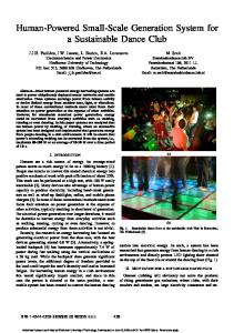
Fig. 1. ROADM node architecture. OT denotes optical transponder. REGEN denotes for 3R regenerator. WSS is a wavelength-selective switch. All links are bidirectional.

II. N ETWORK AND S ERVICE M ODEL GRIPhoN testbed consists of reconfigurable optical adddrop multiplexers (ROADM) as nodes and dense wavelength division multiplexer (DWDM) fibers as links. Wavelength tunable optical transponders (OT) and 3R regenerators (REGEN) are installed at ROADM’s add/drop ports. The network is bidirectional. Figure 1 shows the architecture of a ROADM node. ROADM add/drop ports are engineered “colorless” and “steerable” using optical cross-connects such that all OTs and REGENs can connect to any available wavelengths in any ROADM DWDM port. A backbone wavelength connection is set up between a pair of OTs installed at source and destination ROADM nodes. The GRIPhoN testbed is able to create a new connection automatically in a few minutes. The customer network equipments access the network through the OT interfaces. The route must be a simple path (no node or link is visited twice). If the connection distance exceeds the maximal optical reachability for the network system, some intermediate nodes serve as “regen” nodes and cross-connect the connection to pass a 3R REGEN. The route segment between a pair of OTs or REGENs is called an “optically transparent segment”. A route must keep the same wavelength within a segment but can use a different wavelength after a REGEN is passed. Physically, a 3R REGEN is equivalent to a pair of optical OTs whose customer-side ports are short-connected. However, a REGEN does not have customer-side ports so it cannot be used as an OT. Reachability is the maximal distance of an optically transparent segment allowed for a system. For 10Gbps or 40Gbps systems, reachability is typical 1500km (932 mi). A virtual link graph provides an easy solution to manage the routing of optically transparent segments with reachability constraints. The original virtual link idea appears in [7] as express links. The idea is to create a virtual link for every reachable optical transparent segment. All virtual links that pass the same physical link share the wavelength resource of the physical link. If there is a routing request between two nodes, the route is setup on the virtual link graph. The route must be a simple path that no virtual link in the path shares the same physical link and no node is visited twice. A REGEN is needed at the node that connects two virtual links.

With the dynamic wavelength service, each customer owns or leases a set of OT ports as their top-level network resources. They can choose to connect between their OTs at different nodes in arbitrary ways. However, every connection requires one of the customer’s OTs at each end of the connection. Many customers can run on the same network. But one customer is not allowed to connect to another customer’ OT ports. In this paper, no sharing of network resources is considered between customers. The demands of each customer are independent of the others. The network provider must provide enough network resources to support any possible customer network topology. The network resources, such as REGENs and wavelengths, must be pre-installed so that the customers can reconfigure their OT connections at any time and within a few minutes. The capital expenses of a ROADM network consist of the cost of OTs, REGENs, ROADM ports, and DWDM fiber spans. Since the cost of tunable OT/REGEN is relatively high and increases linearly with the load of network connections, they are counted as a per-equipment cost. Other equipment is modelled as common cost and prorated for every wavelength per mile. In this paper, we use 100 for the normalized cost of a 40Gbps OT, 150 for a 40Gbps REGEN, and 0.07 for the relative common cost per wavelength per mile. Since the end OT ports cost are fixed per customer (prior to joining the network), the cost of OTs are not included in our optimization. Regenerators and the common equipment that are provided by the network provider are the key cost factors that vary with network topologies and customer demands. III. P ROBLEM D ESCRIPTION In this section, we formulate the problem as an integer-linear program (ILP). We show that finding an optimal solution is impractical given the size and structure of the problem. All notation is summarized in Table I. In a ROADM network of a set of nodes N , the customer has a fixed number of OT ports at each node, denoted by On , where n ∈ N . The customer is allowed to connect between nodes freely when spare ports are available. We use E to denote the set of physical DWDM links. The set of virtual links is denoted by V. A virtual link is a set of optical bypassing physical links. Each physical e ∈ E associates with a distance le in miles. Each virtual link also associates with a distance value that is the sum of distance values of all member physical links. A customer demand is defined to be a node to node bidirectional connection, which requires an OT port at each node. If there is more than one connection between a node pair, each connection is modelled as a distinct demand. A port constraint of a customer is the maximal number of connections allowed at each node in the network. A demand matrix for a customer is a set of demands that satisfy the port constraint of the customer. A demand is allocated if at least one route is available in the network to connect it. A demand matrix is satisfied if all member demands can be allocated concurrently. A dimensioned network for a customer is a network allocated

TABLE I N ETWORK NOTATION N E V W l On We,w Rn D S Ds ds,t Pd p CC RC C(·) Xp,d A A A(d) Aw

Node set. Physical link set. Virtual link set. Wavelength set (1 to |W) in a DWDM fiber. Distance for link v ∈ V, e ∈ E. Number of OT ports at node n ∈ N . Binary indicator. We,w = 1 if wavelength w ∈ W is allocated on link e ∈ E, We,w = 0 otherwise. Non-negative integer for the number of REGENs at node n. Set of valid demand matrices. Set of reduced demand matrices. The sth demand Matrix. Ds ∈ D. The tth demand of the sth demand matrix. ds,t = {Nd = (i, j), s, t|i 6= j ∈ N } ∈ Ds . Set of routes for demand d. Sometimes, (i, j) can represent a demand if the order information s, t is not necessary. Route. p = {Vp , Np }, where Vp is set of virtual links and Np is set of regen nodes. Common cost per wavelength per mile. Regenerator cost per equipment. Cost computation function. Binary indicator. Xp,d = 1 if route p ∈ Pd is selected for demand d, Xp,d = 0 otherwise. Route allocation that defines the route for each demand without wavelength assignment. |A| is the number of all demands. A[x : y] represents the list of xth to yth demand-route tuples. Set of all possible route allocations without wavelength assignment. Route allocation for demand d in allocation A. Wavelength assignment for route allocation A ∈ A. A set of solved Xp,d s.

with enough wavelength capacity and REGEN devices to satisfy all possible demand matrices for the customer. A dimensioned network is described by (We,w , Rn ), ∀e ∈ E, w ∈ W, n ∈ N . W is the set of wavelengths available in a DWDM fiber. We,w is a binary variable indicating if wavelength w on physical link e is allocated. Rn is a nonnegative integer for the number of allocated REGENs at node n. In this paper, we assume that the number of wavelengths and REGENs allocated are always smaller than the capacity. A route p includes a set of virtual links along with wavelength assignment information (Vp ) and a set of regen nodes (Np ). The cardinality of Vp is the number of transparent segments in the path. If a route has three segments, the route is represented by p = {Vp = {(v1 , w1 ), (v2 , w2 ), (v3 , w3 )}, Np = {n1 , n2 }}, where v1 ∩ v2 = v1 ∩ v3 = v2 ∩ v3 = ∅, n1 6= n2 given simple path constraints. A demand matrix is a possible set of concurrent connections that may be requested from the customer. Sharing of network resources is allowed between demands of different demand matrices since they are different sets of concurrent connection requests. However, no resource sharing is allowed within a demand matrix. Let Pd be the set of all possible routes for demand d, regardless of resource availability. On a dimensioned network, for each demand matrix D ∈ D, route must be available for each demand d ∈ D simultaneously. A customer can have many possible dimensioned networks. The resource optimization problem is to find a route wavelength assignment for each demand that produces a dimensioned network with minimal cost. The cost objective function

for the network is defined by Equation 1. X X X minimize CC We,w le + RC Rn e∈E w∈W

(1)

n∈N

Optimization is subject to the following constraints. Equation 2 is the constraint for demand matrix validity. I{·} is an indicator function, which is 1 if the condition is met or 0 if not. X ∀D ∈ D, ∀n ∈ N , I{n∈Nd } ≤ On (2) d∈D

Let the binary value Xp,d be the indicator for whether a route p ∈ Pd is picked for demand d. There is one route available for each demand. X Xp,d = 1 (3) ∀D ∈ D, ∀d ∈ D, p∈Pd

Equation 4 prevents wavelength sharing within the same demand matrix. ∀e ∈ E, ∀w ∈ W, ∀D ∈ D, X X I{(v,w)∈Vp ,e∈v} Xp,d ≤ We,w

(4)

d∈D p∈Pd

Equation 5 prevents REGEN sharing within the same demand matrix. X X I{n∈Np } Xp,d ≤ Rn (5) ∀n ∈ N , ∀D ∈ D, d∈D p∈Pd

IV. D EMAND M ATRIX R EDUCTION In this section, we develop techniques to reduce the number of demand matrices used for optimization. With a quick observation, a large number of demand matrices can be included in other demand matrices. For example, assume the port constraints for three nodes are O0 = 2, O1 = O2 = 1. We can show that, if a demand matrix D = {(0, 1), (0, 2)} is satisfied, demand matrices D1 = {(0, 1)}, D2 = {(0, 2)} that are included in D must also be satisfied. Therefore, we do not need to consider D1 or D2 if D is considered. A maximal demand matrix is a demand matrix such that no more demands can be added to the demand matrix without removing an existing demand. We can further reduce the number of demand matrices by leveraging the spare OTs in one demand matrix as REGENs and try to use another demand matrix to cover the demand matrix. A reduced demand matrix is defined for a maximal demand matrix that cannot be further reduced. S ⊆ D is denoted as the set of reduced demand matrices. Figure 2 shows an example. The port numbers on three nodes are O0 = O1 = O2 = 2. The maximal demand matrix D1 = {(0, 1), (0, 1)} is illustrated graphically by two links between node 0 and 1. The maximal demand matrix D2 = {(0, 1), (0, 2), (1, 2)} is also illustrated graphically. D1 is reduced into D2 by mapping the blue demand in D1 to the blue demand in D2 and mapping the red demand in D1 to the red demands in D2 . The two spare OTs at node 2 for demand D1 are connected as a REGEN to make the connection for

the red demand. If D2 is satisfied, We can connect the blue demand on the allocated route of the same blue demand in D2 and connect the red demand on the allocated routes of the two red demands in D2 . The routes for the red demands are connected at node 2 by pairing the spare two OTs that are not used in D1 . Since we pair the two OTs as a REGEN, the two routes can be connected regardless of total distance and wavelength colors. Therefore, D1 is also satisfied. A maximal demand matrix can only be reduced if it has at least two spare OTs at one node (and only at one node, according to the definition of maximal demand matrix). Therefore, if a reduced demand matrix finds a route allocation, all demand matrices that can reduce into it can use the same allocation, except that some reduced demands may need to regenerate route using spare OTs. In fact, the reduction idea leverages spare OTs in some demand matrices as REGENs in order to shrink both the total resource cost and the optimization space. With this technique, fewer demand matrices are considered for optimization, but the optimal result stays the same. The reduction reduces the number of demand matrices by another order of magnitude relative to the number of maximal demand matrices (see Figure 7). V. L OWER B OUND C OMPUTATION Finding an optimal solution for the ILP problem is challenging because of the problem size and structure. The problem is a discrete combinatorial optimization problem. Complex sharing relationships between demand matrices make it difficult to trim the search space. The dimension of Xp,d grows exponentially in the network size and customer ports. The number of virtual links grow linearly in the number of routes per pair that grows exponentially in the size of the physical network. Therefore, the number of available virtual routes for a demand can grow tetrationally in the size of the physical graph. On the dimension of demands d, the number of demand matrices after reduction may also grow exponentially in the number of ports and nodes controlled by the customer. Finding a useful lower bound that is easy to compute is more interesting in practice. For this problem, we can compute the minimal resource cost Cmin (D) for each demand matrix D independently. The maximum of Cmin (D)s is the necessary cost to support all these Ds and thus a lower bound for the problem. Since the demands of the same demand matrix cannot share wavelength capacity, the total cost is additive to the cost of the route of each demand. To find the minimal cost of each D, we simply choose the least cost route for all its demands. The algorithm for finding the lower bound (lowBound) is omitted. The lowBound algorithm is polynomial time in the number of reduced demand matrices and network size. Although the number of reduced demand matrices grows exponentially in some cases, the complexity has been greatly reduced compared to the original optimization problem. However, we do not in general expect the lower bound is achievable.

Function assignWavelength Assign wavelengths to a permutation.

1 2 3

4 5 6 7 8

Input: Virtual link and demand list L Input: List permutation l Output: Wavelength assignment Aw l foreach element (v, d, ∅) ∈ L iterated in the order of l do foreach wavelength w from 1 to |W| do /* Maximize sharing by using the same iteration order */ if w on all physical link e ∈ v is yet not assigned to any other demand in the same demand matrix then /* Demands in the same demand matrix cannot share wavelengths on the same physical link. */ w Assign wavelength Aw l ← Al ∪ {(v, d, w)}; break; end end end

VI. H EURISTIC O PTIMIZATION In this section, we introduce heuristic optimization algorithms to find the minimum cost. For this particular problem, we decompose the entire problem into a wavelength assignment problem and a route allocation problem. Basically, we pick a virtual graph route without wavelength assignment for every demand. The aggregation of all demand-route pairs is called a route allocation. Let A be the set of all possible route allocations without wavelength assignment. For each allocation, we find the minimum cost wavelength assignment Aw . Aw is in fact a set of solved Xp,d s. The cost of Aw , a.k.a C(Aw ), can be computed by Equation 1, where We,w and Rn,r are obtained by substituting the solved Xp,d into Equation 5 and Equation 4. Finally, we pick the route allocation that generates the minimal cost. The decomposition enables us to understand the problem structure better and to trim the space faster in heuristic optimizations. A. Wavelength Assignment Given the set of route allocation for all demands, trying the combination of all wavelengths for each route is not an efficient solution. Especially only a few wavelengths is needed on each link when the traffic demand is low. Instead, we apply a “first-fit” wavelength assignment strategy to an arranged list of virtual link and demand tuples. For each virtual link in the route to which the demand is assigned, a tuple is created. The tuple is a wavelength assignment unit. We use virtual links because a route can have different wavelengths on each virtual link segment. The order of the tuples can be permuted. Each permutation determines wavelength assignment priority for each tuple. Without loss of generality, we fit the wavelength from left to right in the list. The rule of fitting is to choose the lowest wavelength possible for a tuple that has not been assigned to another tuple whose virtual link includes the same physical link(s) and whose demand is of the same demand matrix. The wavelength assignment for a permutation is explained in Function assignWavelength. Figure 3 illustrates an example. Route 1 uses two virtual links, v1 and v2 . Route 2 uses virtual link v3 . Route 3

D1 0

v3 1

two spare OTs

chromosome

v2

father

route 2 (v3) for demand d0,1 mother uniform random crossing point

used as REGEN

Reduce maximal demand ma-

child mate

2

v4

Fig. 2. trices.

route 1 (v1, v2) for demand d0,0

0

reduce 2

1

v1

D2

route 3 (v4) for demand d1,0

Fig. 4. Illustration of mating algorithm used in Fig. 3. Wavelength assignment for three demand-routes. GaOptimize. Relevant virtual links are marked with numbers.

uses virtual link v4 . Three demands, noted by ds,t , are from two demand matrices. Route 1 is allocated to demand d0,0 . Route 2 is allocated to demand d0,1 . Route 3 is allocated to demand d1,0 .We can create four tuples with empty wavelength assignment: t1 = (v1 , d0,0 , ∅), t2 = (v2 , d0,0 , ∅), t3 = (v3 , d0,1 , ∅), t4 = (v4 , d1,0 , ∅). t1 , t3 must not share wavelength because they overlap the demand matrix and the physical link. If the wavelength assignment accords to a list order t1 , t2 , t3 , t4 , assignWavelength gives the result: t1 = (v1 , d0,0 , 1), t2 = (v2 , d0,0 , 1), t3 = (v3 , d0,1 , 2), t4 = (v4 , d1,0 , 1). t4 cannot share wavelength with t3 because of first fit rule. However, if we assign t3 first and use the permutation t3 , t1 , t2 , t4 , the algorithm can provide the optimal result as t3 and t4 share a wavelength. We developed a simulated annealing version to solve the problem heuristically. We define a permutation of the virtual link demand list be a solution. A neighbor solution is created by swapping any two elements. Depending on the temperature and the new cost, we decide if moving to the neighbor for the next iteration or not. Procedure SaWaveAssign explains the details. The temperature drop schedule is determined experimentally. From our experience, the solution is not sensitive to minor changes of the schedule. Proof that some permutation order results in an optical solution is done but left out for space reasons. B. Route Allocation Genetic algorithms are able to quickly explore demandroute combinations by generating a group of route allocations at each generation. These allocations are evaluated and merged for the next generation. Procedure GaOptimize shows the algorithm. Each demand-route tuple represents a gene. The route set for the demand represents all possible choices for this gene. A route allocation of all demands represent a chromosome. A chromosome also maps to a solution. A set of chromosomes forms a generation. In our implementation, a generation is represented by a list of solution and cost tuples. The first generation is a set of randomly picked allocations. Further generations are created by mating chromosomes from the previous generation. The mating candidate is picked using probabilities proportional to the inverse of the chromosome’s cost value. Therefore, low cost solutions are more likely to pass to the next generation while high cost solutions still have some chance to get picked. Two chromosomes mate in a probability of a crossover rate. Mating combines a random upper half of the father’s chromosome and random lower half

Procedure SaWaveAssign Simulated annealing wavelength assignment for route allocation.

1 2 3 4 5 6 7 8 9 10 11 12 13 14 15

16 17 18 19 20 21 22 23 24 25 26 27 28

Input: Allocation A for all demands Input: Optimization steps k Output: Optimal wavelength assignment Aw Empty list L ← ∅; foreach demand d ∈ D ∈ S do Get the route allocation p ← A(d); foreach virtual link v ∈ p do Create a link demand tuple (v, d, ∅); L ← L ∪ {(v, d, ∅)}; end end /* Initial wavelength assignment */ Get permutation l by sorting L at the descending order of the physical links and distance in v; Aw l ← assignWavelength(L, l); /* Compute the lower bound */ Get lower bound Clb ← lowBound(); Get initial cost c ← C(Aw l ); Initialize minimum cost cm ← c; /* Temperature schedule */ Set start temperature T ← 10c; /* Start temperature is set 10 times the initial cost. */ Set minimal temperature Tm ← 0.0001; /* It is extremely unlikely to move to a worse neighbor at this temperature. */ m ; Linear temperature drop step ∆T ← T −T k while k > 0 and c > Clb do Create a new permutation l′ by swap the order of two uniform picked tuples in l; Aw ← assignWavelength(L, l′ ); l′ New cost c′ ← C(Aw ); l′ if c′ < cm then ′ c←c; l ← l′ ; /* Save the new minimum */ cm ← c′ ; w w A ← Al′ ; else Get a uniform random real number x ∈ [0, 1); c′ −c

if e− T > x then /* Move to the neighbor. If c′ < c, always move. */ c ← c′ ; l ← l′ ; end

29 30 31 32 end 33 Update temperature T ← max(T − ∆T, Tm ); 34 Update steps k ← k − 1; 35 end

of the mother’s chromosome. Figure 4 illustrates the mating algorithm. If two chromosomes do not mate, the father’s chromosome is used. Each gene of the child is subjected to mutation according to a mutation rate. If a gene is selected

Procedure GaOptimize Genetic algorithm optimization.

1 2 3 4

5 6 7 8 9 10 11 12 13 14 15 16

17 18 19 20 21 22 23 24 25 26 27 28 29 30 31 32 33 34 35 36 37 38 39 40 41 42

Input: all demands d ∈ D ∈ S Input: Generations k Input: Population per generation s Input: Optimization steps for wavelength assignment k′ Output: Optimal allocation and wavelength assignment Aw Crossover rate α ← 0.6; Mutation rate β ← 0.001; /* Compute the lower bound */ Get lower bound Clb ← lowBound(); Initialize minimum cost cm ← ∞; /* Generate a random generation of s allocations */ for i from 1 to s do foreach demand d ∈ D ∈ S do Ai (d) ← p where p is uniform randomly picked in Pd ; end ′ Get the wavelength assignment Aw i ← SaWaveAssign(Ai , k ); Compute cost ci ← C(Aw i ); if ci < cm then /* Record the minimum cost */ cm ← ci ; Aw ← A w i ; end end while k > 0 and cm > Clb do /* Generate a new generation of s allocations */ for i from 1 to s do /* Mating algorithm */ s Get the father m ← rouletteWheelPick({(Aw i , ci )} ); s Get the mother n ← rouletteWheelPick({(Aw i , ci )} ); Get a uniform random real number r ∈ [0, 1); if r > α then Get a uniform random integer a ∈ (1, |Am |); Create a child by merge two parents A′i ← Am [1 : a] + An [a + 1 : |Am |]; else Copy the father to the child Ai ← Am ; end /* Mutation algorithm */ foreach demand d ∈ D ∈ S do Get a uniform random real number r ∈ [0, 1); if r < β then A′i (d) ← p where p is uniformly picked in Pd ; end end Optimal wavelength assignment ′ ′ A′w i ← SaWaveAssign(Ai , k ); Compute cost c′i ← C(A′w ); i if c′i < cm then /* Record the minimum cost */ ′ cm ← ci ; Aw ← A′w i ; end end s ′w ′ s Update the generation {Aw i , ci } ← {Ai , ci } ; Update steps k ← k − 1; end

for mutation, a random route is re-selected for the demand. In the algorithm, the crossover rate is fixed at 0.6. The mutation rate is fixed at 0.001. The algorithm is not sensitive to minor changes in these numbers. C. Route Space Reduction Even though we use heuristic optimization techniques, the number of routes for each demand is still too large on our testing network (Figure 5) to find good solutions fast.

Therefore, we need further heuristic route space reduction to effectively exclude bad solutions. 1) Route Cost Limit: Unless for extremely cases, excessively expensive routes are unlikely included in the optimal solution. However, searching too few routes can affect the quality of the results. On CORONET, we found it a good trade-off of efficiency and quality to limit the search space of routes for each demand within 1.4 times the cost of the least cost route of the demand. 2) Fixed Route per Node Pair: Even if two demands have the same end nodes, they can use different routes. However, in practise, optimizing routes per demand can be extremely expensive on a larger network, where the nodes are more distant and route choices are many. If we use only one route per node pair, the search space is greatly reduced. In fact, we find that the optimizer is able to land a good enough solution much faster when using a fixed route per node pair. We developed a fixed-route version of GaOptimize to exploit this heuristic. The improved algorithm retains its structure except for the changing concept of genes and chromosomes. Demands can no longer choose their routes as freely as before. Node pairs are the unit to map routes. We define a new tuple called pair-route, which maps a route for each node pair. Each pair-route tuple represents a gene. The route set for the pair represents all possible choices for this gene. A route allocation of all pairs represent a chromosome. Since the route for each demand is determined by the node pair, a chromosome also maps to a solution. A set of chromosomes forms a generation. Extending GaOptimize to support fixed routes per pair is straightforward, so we omit the algorithm from this paper. VII. N UMERICAL R ESULTS CORONET is created by Telcordia-AT&T team to mimic a typical large international core network [3]. We use the U.S. contiguous part of CORONET that consists of 75 nodes and 99 links. Each node maps to a U.S. city. Figure 5 shows the topology of the network. The link numbers are marked on the topology. Figure 6 lists the distance of each physical link in miles. We assume a 40Gbps ROADM system deployed to the network. Each DWDM link has 80 wavelengths. The optically transparent reachability is 932 miles. Each REGEN costs 150 and the common cost is 0.07 per mile per wavelength. Three cities are picked as base cities for a customer. They are marked in the figure with red (Chicago), blue (New York City), and green (San Diego). Assume that the default port constraints are Or = 2, Ob = 3, Og = 2. Only the reduced demand matrices are used by the optimizer. We solve each optimization problem using genetic algorithm (GA) and genetic algorithm with fixed routes (GAF). They are all compared with the lower bound (Clb ). The simulation is run on an AMD Opteron 64bit machine with a 2.2GHz CPU, 1MB cache memory, and 7GB main memory. We study the performance of the genetic algorithms by varying the number of generations k and population per generation s. We choose k ′ = 50 for wavelength assignment simulated annealing steps. Only the routes of cost within 1.4

24

2

54 3

Fig. 6. # 0 1 2 3 4 5 6 7 8 9 10 11 12 13 14 15 16 17 18 19 20 21 22 23 24

53

92 26

95 62

25

44

13

14

38

73

74 76

84

87

37

75

36 15 30

78

33 35 91

31

77

32 34

52

97

70

66 57

29 65

71

27

18

56

9

58 67

42

19

90

61

89

22

43

41 40 60

81

83

5

80

79

17

4

7

72

39 0

6

49 47

16 1

69 98 68

59

93

11

48 94

55 8

82 88

10

21

20

96

28

51 50

23

64

46

63

85

86

45 12

mile 252.7 570.9 207.8 175.7 850.1 485.8 327.7 707.7 199.7 329.4 415.6 211.5 107.7 134.4 288.6 50.4 375.1 110.5 546.8 660.0 636.6 264.3 436.9 554.2 59.9

# 25 26 27 28 29 30 31 32 33 34 35 36 37 38 39 40 41 42 43 44 45 46 47 48 49

CORONET link distance. mile 252.3 95.0 284.5 322.6 119.9 344.4 124.0 268.2 144.9 133.1 582.8 179.2 143.4 221.0 324.6 415.5 275.2 690.3 548.5 80.4 723.3 379.3 372.2 290.0 217.5

# 50 51 52 53 54 55 56 57 58 59 60 61 62 63 64 65 66 67 68 69 70 71 72 73 74

mile 517.8 98.3 238.4 139.7 94.2 184.9 235.5 353.2 313.8 371.9 525.0 196.0 22.0 167.9 113.0 221.3 355.3 283.4 297.8 97.4 426.3 421.0 490.0 18.2 149.7

# 75 76 77 78 79 80 81 82 83 84 85 86 87 88 89 90 91 92 93 94 95 96 97 98

mile 153.1 102.1 224.0 287.8 99.5 851.8 19.3 145.0 206.8 145.1 431.0 166.8 355.2 703.3 915.9 209.3 142.6 109.0 57.9 335.2 167.8 333.2 108.0 295.6

Fig. 5. U.S. CORONET topology with node and link numbers. Geographic information is removed for clarity.

times the least cost route for each node pair are considered. Figure 8 shows the cost color map of the optimized cost of GAF. Cooler colors indicate better solutions, which occur with increasing number of generations and population. Using k = 80 generations, s = 3000 populations, the values are good enough and the runtime is about an hour on our machines. We compare the performance of all algorithms using a four-node demand constraints Or = 2, Ob = 3, Og = 24, Ox = 1, x ∈ N . The fourth node is an arbitrary node in the network. If x is the same node as the red, blue or green one, there are still 3 nodes except for one having an additional port. We choose the parameters s = 3000, k = 80, k ′ = 50 for GA/GAF so every test case walks the same number of samples in the space and runs approximately for an hour. The comparison is shown in Figure 9. All the nodes are sorted in the increasing order of the lower bound for each test case. The results for red, blue and green nodes are annotated. If x is the red, blue or green node, there is only one reduced demand matrix, and the optimal result equals the lower bound. On average, GAF requires 10% additional cost over the lower bound. GA requires 26% additional overhead. VIII. R ELATED W ORK Wavelength assignment and regenerator placement problems on wavelength translucent networks have been extensively studied. The regenerator placement problem with given routes or without given routes are NP-hard [8]. Previous studies focused on different traffic models. Several heuristic regenerator placement algorithms was proposed for dynamic Poisson traffic [9]. The authors in [8], [10] proposed an ILP formulation to compute optical regenerator placement for static demands. The authors in [11] studied the reduction of electrooptical equipment cost relative to the increase of reachability in the network for a given traffic demand. More heuristic

regenerator placement algorithms were proposed in [12] to reduce the blocking for dynamic Poisson traffic. A resource optimization problem for subwavelength grooming to support multiple possible static traffic matrices was studied in [13]. However, the paper focused on a different problem that is to minimize OTs and lightpaths at the electronic layer. The routing and wavelength assignment problem has long been known to be NP-hard [14], but many heuristic algorithms have been proposed [15]–[18]. Previous studies also suggested that routing algorithms have a higher impact on the performance than wavelength assignment [19]. Specific wavelength assignment techniques can reduce the impact of cross-talk so as to increase the reachability of some routes [20]. These techniques are not mature in near-future devices. A recent work [7] propose an efficient approach that simplifies routing, wavelength assignment and regenerator placement using express links on translucent networks. Combinatorial optimization problems can quickly become unmanageable when the number of choices is large. Simulated annealing [21], [22] is a practical heuristic optimization tool to find a good solution reasonably quickly. The algorithm simulates the random walk of atoms in a metal that is heated and slowly cooled. Genetic algorithms [23] apply the idea of natural selection to find an optimal combination of elements. The approach has been found useful for discrete and unstructured problems. However, for each specific problem that applies simulated annealing or genetic algorithms, the solution elements must be carefully structured and algorithm parameters tuned to achieve the best performance. IX. C ONCLUSION This paper introduces a new network optimization problem for dynamic wavelength services on future reconfigurable

5000

total max reduced

4500 GAF cost

100

1000

100

10

90

5000

80

4800

70

4600

60

4400

50

4200

40 30 20

1 1

2

3 4 O0=O1=O2=O3=x

5

6

7

8 9 10

5200

10

3500 3000

2000 1500

3800

1000

500 1000 1500 2000 2500 3000 3500 4000 4500 5000 population s

green

2500

4000

3600 0

4000

minimum cost

10000

generations k

number of demand matrices

100000

red

blue

GA GAF Clb

500 0 additional node x

Fig. 7. Semi-log plot for the number of total, maximal, and reduced demand matrices for four nodes with the same number of ports: O0 = O1 = O2 = O3 = x. All numbers grow exponentially in the number of ports.

Fig. 8. GAF cost color map for Or = 2, Ob = 3, Og = 2. Clb = 2595.23. Each data point is an independent optimization process.

networks. In order to solve this challenging problem with practically available computing resources, we propose a demand matrix reduction technique and a heuristic optimizer. The demand matrix reduction algorithm can reduce the number of inputs for the optimization problem by an order of magnitude. The heuristic optimizer includes a simulated annealing-based wavelength assignment optimizer and a genetic algorithmbased route allocation optimizer. We also find a useful lower bound of the optimal cost that is efficient to compute. We find that, given a small amount of computing power, limiting the route space for fixed route per node pair (GAF) outperforms the unlimited version (GA). Compared to a lower bound, on average GAF requires only 10% additional cost on an experimental backbone optical network of realistic scale and size. R EFERENCES [1] R. Doverspike, “Practical aspects of bandwidth-on-demand in optical networks,” Panel on Emerging Networks, Service Provider Summit, Optical Fiber Communication Conference (OFC), Anaheim, CA, Mar. 2007. [2] K. Oikonomou and R. Sinha, “Network design and cost analysis of optical vpns,” in OFC 2006 - Optical Fiber Communication Conference and Exhibit, Mar. 2006. [3] A. L. Chiu, G. Choudhury, G. Clapp, R. Doverspike, J. W. Gannett, J. G. Klincewicz, G. Li, R. A. Skoog, J. Strand, A. von Lehmen, and D. Xu, “Network Design and Architectures for Highly Dynamic Next-Generation IP-Over-Optical Long Distance Networks,” Journal of Lightwave Technology, vol. 27, pp. 1878–1890, Jun. 2009. [4] J. Strand and A. Chiu, “Realizing the advantages of optical reconfigurability and restoration with integrated optical cross-connects,” Journal of Lightwave Technology, vol. 21, no. 11, pp. 2871–2882, Nov 2003. [5] M. D. Feuer, D. C. Kilper, and S. L. Woodward, Optical Fiber Telecommunications. London, UK: Elsevier Inc., 2008, vol. B: Systems and Networks, ch. ROADMs and their system applications. [6] X. J. Zhang, M. Birk, A. Chiu, R. Doverspike, M. D. Feuer, P. Magill, E. Mavrogiorgis, J. Pastor, S. L. Woodward, and J. Yates, “Bridgeand-roll demonstration in GRIPhoN (globally recongurable intelligent photonic network),” in Optical Fiber Communication Conference and Exposition (NFOEC’10), San Diego, California, USA, Mar. 2010. [7] G. Li, A. Chiu, R. Doverspike, D. Xu, and D. Wang, “Efficient routing in heterogeneous core DWDM networks,” in NFOEC2010, San Diego, CA, Mar. 2010. [8] M. Flammini, A. Marchetti Spaccamela, G. Monaco, L. Moscardelli, and S. Zaks, “On the complexity of the regenerator placement problem in optical networks,” in SPAA ’09: Proceedings of the twenty-first annual symposium on Parallelism in algorithms and architectures. New York, NY, USA: ACM, 2009, pp. 154–162.

Fig. 9. Comparison of optimization result for Or = 2, Ob = 3, Og = 2, Ox = 1. Each data value is a random optimization run. The nodes are sorted in the increasing order of the lower bound.

[9] S.-W. Kim and S.-W. Seo, “Regenerator placement algorithms for connection establishment in all-optical networks,” IEE Proceedings Communications, vol. 148, no. 1, pp. 25–30, Feb 2001. [10] E. Yetginer and E. Karasan, “Regenerator placement and traffic engineering with restoration in GMPLS networks,” Photonic Network Communications, vol. 6, pp. 139–149(11), Sep. 2003. [11] A. Morea, H. Nakajima, L. Chacon, E. Le Rouzic, B. Decocq, and J.-P. Sebille, “Impact of the reach of WDM systems and traffic volume on the network resources and cost of translucent optical transport networks,” in Sixth International Conference on Transparent Optical Networks, vol. 1, July 2004, pp. 65–68. [12] X. Yang and B. Ramamurthy, “Sparse regeneration in translucent wavelength-routed optical networks: Architecture, network design and wavelength routing,” Photonic Network Communications, vol. 10, no. 1, pp. 39–53, Jul. 2005. [13] N. Srinivas and C. S. R. Murthy, “Design and dimensioning of a WDM mesh network to groom dynamically varying traffic,” Photonic Network Communication, vol. 7, no. 2, pp. 179–191, Mar. 2004. [14] H. Zang, J. P. Jue, and B. Mukherjee, “A review of routing and wavelength assignment approaches for wavelength-routed optical WDM networks,” Optical Networks Magazine, vol. 1, pp. 47–60, 2000. [15] A. Birman and A. Kershenbaum, “Routing and wavelength assignment methods in single-hop all-optical networks with blocking,” INFOCOM ’95. Fourteenth Annual Joint Conference of the IEEE Computer and Communications Societies. Bringing Information to People. Proceedings. IEEE, pp. 431–438 vol.2, Apr 1995. [16] X. Zhang and C. Qiao, “Wavelength assignment for dynamic traffic in multi-fiber WDM networks,” in 7th International Conference on Computer Communications and Networks, Oct 1998, pp. 479–485. [17] C. Assi, A. Shami, M. Ali, R. Kurtz, and D. Guo, “Optical networking and real-time provisioning: an integrated vision for the next-generation internet,” Network, IEEE, vol. 15, no. 4, pp. 36–45, Jul/Aug 2001. [18] L. Li and A. Somani, “Dynamic wavelength routing techniques and their performance analyses,” in Optical WDM Networks: Principles and Practice, K. M. Sivalingam and S. Subramaniam, Eds., Oct. 2002, pp. 247–272. [19] H. Zang, J. Jue, L. Sahasrabuddhe, R. Ramamurthy, and B. Mukherjee, “Dynamic lightpath establishment in wavelength routed WDM networks,” Communications Magazine, IEEE, vol. 39, no. 9, pp. 100–108, Sep 2001. [20] J. He, “RWA algorithm design and performance analysis for all-optical networks subject to physical impairments,” Ph.D. dissertation, University of Virginia, May 2008. [21] S. Kirkpatrick, C. D. Gelatt, Jr., and M. P. Vecchi, “Optimization by simulated annealing,” Science, vol. 220, pp. 671–680, 1983. [22] R. Carr, “Simulated annealing,” MathWorld–A Wolfram Web Resource, created by Eric W. Weisstein http://mathworld.wolfram.com/SimulatedAnnealing.html. [23] H.-P. Schwefel, Numerical Optimization of Computer Models. New York, NY, USA: John Wiley & Sons, Inc., 1981.