Hidden Two-Stream Convolutional Networks for Action Recognition

Hidden Two-Stream Convolutional Networks for Action Recognition Yi Zhu1 Zhenzhong Lan2 Shawn Newsam1 Alexander G. Hauptmann2 1 2 University of California, Merced Carnegie Mellon University

arXiv:1704.00389v1 [cs.CV] 2 Apr 2017

{yzhu25,snewsam}@ucmerced.edu

{lanzhzh,alex}@cs.cmu.edu

Abstract

Spatial Stream CNN

Analyzing videos of human actions involves understanding the temporal relationships among video frames. CNNs are the current state-of-the-art methods for action recognition in videos. However, the CNN architectures currently being used have difficulty in capturing these relationships. State-of-the-art action recognition approaches rely on traditional local optical flow estimation methods to pre-compute the motion information for CNNs. Such a two-stage approach is computationally expensive, storage demanding, and not end-to-end trainable. In this paper, we present a novel CNN architecture that implicitly captures motion information. Our method is 10x faster than a two-stage approach, does not need to cache flow information, and is end-to-end trainable. Experimental results on UCF101 and HMDB51 show that it achieves competitive accuracy with the two-stage approaches.

Temporal Stream CNN

Late Fusion

MotionNet

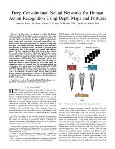
Figure 1. Illustration of proposed hidden two-stream networks. MotionNet takes consecutive video frames as inputs and estimates motion. Then the temporal stream CNN learns to project them to action labels. Late fusion is performed to combine spatio-temporal information. Both streams are end-to-end trainable.

and motion information in two separate CNNs. • Traditional optical flow estimation is completely independent of action recognition and is prone to error. Because it is not end-to-end trainable, we cannot extract motion information that is optimal for the tasks.

1. Introduction The field of human action recognition has changed drastically over the past few years. We have moved from manually designed features [31, 21, 16] to learned CNN features [27, 14]; from encoding appearance information to encoding motion information [24, 32]; and from learning local features to learning global video features [33, 6, 22, 17]. The performance has continued to soar higher as we incorporate more of the steps into the end-to-end learning framework. Nevertheless, the state-of-the-art CNN structures we are using still have difficulty in capturing motion information directly from video frames. We rely on traditional local optical flow estimation methods to compute motion information for the CNNs. This two-stage pipeline is suboptimal for the following reasons:

Our primary aim, therefore, is to move toward end-toend learning by incorporating the optical flow estimation into the CNN framework. We hope that, by taking consecutive video frames as inputs, our CNNs learn the temporal relationships among pixels and use the relationships to predict action classes. Theoretically, given how powerful CNNs are for image processing tasks, it would not make sense to not use them for a low-level task like optical flow estimation. However, in practice, we still face many challenges, the main ones of which are summarized as follows: • We need to train our models without supervision. The ground truth flow required for supervision is usually not available except for limited synthetic data. We can perform weak supervision by using the optical flow calculated from traditional methods. However, the accuracy of these models would be limited by the accuracy of the traditional methods.

• The pre-computation of optical flow is time consuming and storage demanding compared to the CNN step. Even extracted on GPUs, optical flow calculation has been the major speed bottleneck of the current twostream approaches, which learn to encode appearance 1

• We need to train our optical flow estimation models from scratch. The models (filters) learned for optical flow estimation tasks are very different from models (filters) learned for other image processing tasks such as object recognition [19]. Hence, we cannot pre-train our model using other tasks such as ImageNet challenges [4].

representation that is better than optical flow. Therefore, we believe that end-to-end training is a better solution than a two-stage approach. Before we introduce our new method in detail, we provide some background on our work in this paper.

• We cannot simply use the traditional optical flow estimation objective functions. We are concerned chiefly with how to learn optical flow for action recognition. Therefore, our optimization goal is more than just minimizing the endpoint errors (EPE) [7, 38].

The field of human action recognition has changed drastically over the past few years. Initially, traditional handcrafted features such as Improved Dense Trajectories (IDT) [31, 16] dominated the field of video analysis for several years. Despite their superior performance, IDT and its improvements [16, 21] are computationally formidable for real applications. CNNs [14, 11, 27], which are often several orders of magnitude faster than IDTs, performed much worse than IDTs in the beginning. This inferior performance is mostly because CNNs have difficulty in capturing motion information among frames. Later on, two-stream CNNs [24, 32] address this problem by pre-computing the optical flow using traditional optical flow estimation methods [36] and training a separate CNN to encode the pre-computed optical flow. This additional stream (a.k.a., the temporal stream) significantly improved the accuracy of CNNs and finally allowed them to outperform IDTs on several benchmark action recognition datasets [32, 33]. These accuracy improvements indicate the importance of temporal motion information for action recognition as well as the inability of existing CNNs to capture such information. However, compared to the CNN step, the optical flow calculation step is computationally expensive. It is the major speed bottleneck of the current two-stream approaches. As an alternative, Zhang et al. [37] proposed to use motion vectors, which can be obtained directly from compressed videos without extra calculation, to replace the more precise optical flow. This simple improvement brought more than 20x speedup compared to the traditional two-stream approaches. However, this speed improvement came with an equally significant accuracy drop. The encoded motion vectors lack fine structures, and contain noisy and inaccurate motion patterns, leading to much worse accuracy compared to the more precise optical flow [36]. These weaknesses are fundamental and can hardly be improved. Another more promising approach is to learn to predict optical flow using supervised CNNs, which is closer to our approach. There are two representative works in this direction. Ng. et al. [19] used optical flow calculated by traditional methods as supervision to train a network to predict optical flow. This method avoids the pre-computation of optical flow at inference time and greatly speeds up the process. However, as we will demonstrate later, the quality of the optical flow calculated by this approach is limited by the quality of the traditional flow estimation, which again limits its potential on action recognition. The other representative

2. Related Work

To address these challenges, we first pre-train a CNN with the goal of generating optical flow from a set of consecutive frames. Through a set of specially designed operators and unsupervised objective functions, our new pretraining step can generate optical flow that is similar to that generated by one of the best traditional methods [36]. As illustrated in Figure 1, we call this pre-trained network as MotionNet. Given the MotionNet, we concatenate it with a temporal CNN that projects the estimated optical flow to the target action labels. We then fine-tune this stacked temporal stream CNN in an end-to-end manner with the goal of predicting action classes for the input frames. Our end-to-end stacked temporal stream CNN has multiple advantages over the traditional two-stage approach: • First, it does not require any additional label information hence there are no upfront cost. • Second, it is computationally much more efficient. It is about 10x faster than traditional approaches. • Third, it is much more storage efficient. Due to the high optical flow prediction speed, we do not need to pre-compute optical flow and store it on disk. Instead, we predict it on-the-fly. • Last but not least, it has much more room for improvement. Traditional optical flow estimation methods have been studied for decades and the room for improvement is limited. In contrast, our end-to-end and implicit optical flow estimation is completely different as it connects to the final tasks. Although currently we only get accuracies that are close to the two-stage approaches, we believe that we are far from exploiting the full potential of this new framework. We call our new two-stream approach hidden two-stream CNNs as it implicitly generates optical flow. It is important to distinguish between these two ways of introducing motion information to the encoding CNNs. Although optical flow is currently being used to represent the motion information in the videos, we do not know whether it is an optimal representation. There might be an underlying motion 2

Name conv1 conv1 1 conv2 conv2 1 conv3 conv3 1 conv4 conv4 1 conv5 conv5 1 conv6 conv6 1 flow6 (loss6) deconv5 xconv5 flow5 (loss5) deconv4 xconv4 flow4 (loss4) deconv3 xconv3 flow3 (loss3) deconv2 xconv2 flow2 (loss2) flow2 norm conv1 1 vgg conv1 2 vgg pool1 vgg conv2 1 vgg conv2 2 vgg pool2 vgg conv3 1 vgg conv3 2 vgg conv3 3 vgg pool3 vgg conv4 1 vgg conv4 2 vgg conv4 3 vgg pool4 vgg conv5 1 vgg conv5 2 vgg conv5 3 vgg pool5 vgg fc6 vgg fc7 vgg fc8 vgg (action loss)

work is by Ilg et al. [9] and uses the network trained on synthetic data where ground truth flow exists. The performance of this approach is again limited by the quality of the data used for supervision. The ability of synthetic data to represent the complexity of real data is very limited. Actually, in Ilg et al. [9]’s work, they show that there is a domain gap between real data and synthetic data. To address this gap, they simply grew the synthetic data to narrow the gap. The problem with this solution is that it may not work for other datasets and it is infeasible to do this for all datasets. Our work addresses the optical flow estimation problem in a much more fundamental and promising way. We predict optical flow on-the-fly using CNNs, thus addressing the computation and storage problems. And we perform unsupervised pre-training on real data, thus addressing the domain gap problem. Another weakness of the current two-stream CNN approach is that it maps local video snippets into global labels. In image classification, we often take a whole image as the input to CNNs. However, in video classification, because of the much larger size of videos, we often use sampled frames/clips as inputs. One major problem of this common practice is that video-level label information can be incomplete or even missing at frame/clip-level. This information mismatch leads to the problem of false label assignment, which motivates another line of research that tries to do CNN-based video classification beyond short snippets. Ng et al. [20] reduced the dimension of each frame/clip using a CNN and aggregated frame-level information using LSTM. Varol et al. [30] stated that Ng et al.’s approach is suboptimal as it breaks the temporal structure of videos in the CNN step. Instead, they proposed to reduce the size of each frame and use longer clips (e.g., 60 frames vs 16 frames) as inputs. They managed to gain significant accuracy improvements compared to shorter clips. However, the way they reduced the spatial resolution comes at a cost of a large accuracy drop. In the end, the overall accuracy improvement is less impressive. Wang et al. [33] experimented with sparse sampling and jointly train on the sparsely sampled frames/clips. In this way, they incorporate more temporal information while preserving the spatial resolution. Diba et al. [6], Qiu et al. [22], and Lan et al. [17] took a step forward along this line by using the networks of Wang et al. [33] to scan through the whole video, aggregate the features (output of a layer of the networks) using some pooling methods, and fine-tune the last layer of the network using the aggregated features. We believe that these approaches are still sub-optimal as they again break the end-to-end learning into a two-stage approach. However, because these approaches are currently the best at incorporating global temporal information, they represent the current state-of-the-art in this field. In this paper, we do not address the false label problem because we only use the basic two-stream approaches

Kernel 3×3 3×3 3×3 3×3 3×3 3×3 3×3 3×3 3×3 3×3 3×3 3×3 3×3 4×4 3×3 3×3 4×4 3×3 3×3 4×4 3×3 3×3 4×4 3×3 3×3 3×3 3×3 3×3 2×2 3×3 3×3 2×2 3×3 3×3 3×3 2×2 3×3 3×3 3×3 2×2 3×3 3×3 3×3 2×2 3×3 3×3 3×3

Str 1 1 2 1 2 1 2 1 2 1 2 1 1 2 1 1 2 1 1 2 1 1 2 1 1 1 1 1 2 1 1 2 1 1 1 2 1 1 1 2 1 1 1 2 1 1 1

Ch I/O 33/64 64/64 64/128 128/128 128/256 256/256 256/512 512/512 512/512 512/512 512/1024 1024/1024 1024/20 1024/512 1044/512 512/20 512/256 788/256 256/20 256/128 404/128 128/20 128/64 212/64 64/20 20/20 20/64 64/64 64/64 64/128 128/128 128/128 128/256 256/256 256/256 256/256 256/512 512/512 512/512 512/512 512/512 512/512 512/512 512/512 512/4096 4096/4096 4096/M

In Res 224 × 224 224 × 224 224 × 224 112 × 112 112 × 112 56 × 56 56 × 56 28 × 28 28 × 28 14 × 14 14 × 14 7×7 7×7 7×7 14 × 14 14 × 14 14 × 14 28 × 28 28 × 28 28 × 28 56 × 56 56 × 56 56 × 56 112 × 112 112 × 112 112 × 112 224 × 224 224 × 224 224 × 224 112 × 112 112 × 112 112 × 112 56 × 56 56 × 56 56 × 56 56 × 56 28 × 28 28 × 28 28 × 28 28 × 28 14 × 14 14 × 14 14 × 14 14 × 14 7×7 1×1 1×1

Out Res 224 × 224 224 × 224 112 × 112 112 × 112 56 × 56 56 × 56 28 × 28 28 × 28 14 × 14 14 × 14 7×7 7×7 7×7 14 × 14 14 × 14 14 × 14 28 × 28 28 × 28 28 × 28 56 × 56 56 × 56 56 × 56 112 × 112 112 × 112 112 × 112 224 × 224 224 × 224 224 × 224 112 × 112 112 × 112 112 × 112 56 × 56 56 × 56 56 × 56 56 × 56 28 × 28 28 × 28 28 × 28 28 × 28 14 × 14 14 × 14 14 × 14 14 × 14 7×7 1×1 1×1 1×1

Input Frames conv1 conv1 1 conv2 conv2 1 conv3 conv3 1 conv4 conv4 1 conv5 conv5 1 conv6 conv6 1 conv6 1 deconv5+flow6+conv5 xconv5 xconv5 deconv4+flow5+conv4 xconv4 xconv4 deconv3+flow4+conv3 xconv3 xconv3 deconv2+flow3+conv2 xconv2 flow2 flow2 norm conv1 1 vgg conv1 2 vgg pool1 vgg conv2 1 vgg conv2 2 vgg pool2 vgg conv3 1 vgg conv3 2 vgg conv3 3 vgg pool3 vgg conv4 1 vgg conv4 2 vgg conv4 3 vgg pool4 vgg conv5 1 vgg conv5 2 vgg conv5 3 vgg pool5 vgg fc6 vgg fc7 vgg

1

1

1

1

Table 1. Our stacked temporal stream architecture. Top: MotionNet. Bottom: tradtional temporal stream CNN. M is the number of action categories. Str: stride. Ch I/O: number of channels of input/output feature maps. In/Out Res: input/output resolution.

in Wang et al. [32]. Nevertheless, all the methods addressing the false label problem should also be able to improve our method. For example, we can simply replace our network for encoding optical flow from [32] with the one from [33] to get better accuracy.

3. Hidden Two-Stream Networks In this section, we describe our proposed hidden twostream networks in detail. We first introduce our unsupervised network for optical flow estimation along with employed good practices in Section 3.1. We name it MotionNet. In Section 3.2, we stack the temporal stream network upon MotionNet to allow end-to-end training. We call this stacked network stacked temporal stream CNN. In the end, we introduce the hidden two-stream CNNs in Section 3.3 by fusing our stacked temporal stream CNN with the spatial stream CNN.

3.1. Unsupervised Optical Flow Learning We treat the optical flow estimation problem as an image reconstruction problem [35]. Basically, given a frame pair, 3

we hope to generate optical flow that allows us to reconstruct one frame from the other. Formally, taking a pair of adjacent frames I1 and I2 as inputs, our CNN generates a motion field V . Then using the predicted flow field V and I2 , we hope to get the reconstructed frame I10 using inverse warping, i.e., I10 = T [I2 , V ], where T is the inverse warping function. The goal is to minimize the photometric error between I1 and I10 . Our CNN architecture is inspired by the “FlowNet2-SD” network introduced in [9] with some specifically designed objective functions and operators. As will be shown later, these modifications significantly improve the accuracy of our MotionNet. The details of our network can be seen in Table 1, where the top part represents our MotionNet and the bottom part is the traditional temporal stream CNN. We also investigate using VGG16 [25] as our MotionNet contractive architecture because it has a pre-trained model on ImageNet challenges, which may serve as a good initialization. However, it achieves worse results than training from scratch due to the fact that low-level convolution layers learn completely different filters for object recognition and optical flow prediction. The following are the key components and modifications we made to allow us to achieve good performance with MotionNet. First of all, allowing networks to train on low resolution inputs. Because the real data we experimented on has much lower resolution than the synthetic data that “FlowNet2SD” applies to, we remove the first convolution layer that has a large receptive field and reduce the stride of the second convolution layer to be 1. These two changes allow our deep networks to accept much lower resolution images. Second, having multiple losses. We explore three objective functions that help us to generate better optical flow. These objective functions are as follows.

textured regions. It is calculated as: Lsmooth = ρ(∇Vxx ) + ρ(∇Vyx ) + ρ(∇Vxy ) + ρ(∇Vyy ). (2) ∇Vxx and ∇Vyx are respectively the gradients of the estimated flow field V x in the horizontal and vertical directions. Similarly, ∇Vxy and ∇Vyy are the gradients of V y . The generalized Charbonnier penalty ρ(x) is the same as in the pixelwise loss. • A structural similarity (SSIM) object function that helps us to learn the structures of frames. It is calculated as: Lssim =

(3)

SSIM(·) is a standard structural similarity function. Our experiments show that this simple strategy significantly improves the quality of our estimated flows. It forces our MotionNet to produce flow fields with clear motion boundaries. The overall loss of our MotionNet is a weighted sum of the pixelwise reconstruction loss, the piecewise smoothness loss, and the region-based SSIM loss, L = λ1 · Lpixel + λ2 · Lsmooth + λ3 · Lssim

(4)

where λ1 , λ2 , and λ3 weight the relative importance of the different metrics during training. λ1 and λ3 are set to 1. λ2 is set as suggested in [7]. Third, designing small displacement network. This is an improvement made by the original “FlowNet2-SD” network [9]. We found that it is also helpful in our unsupervised settings. Basically, they made the beginning of the network deeper by exchanging the 7 × 7 and 5 × 5 kernels with multiple 3 × 3 kernels. According to [9], it can help to detect small motions. Fourth, inserting convolutional layers between deconvolutional layers. As suggested in [18], we add a convolutional layer between each deconvolution pair in the expanding part to yield smoother motion estimation. In our experiments, we conduct an ablation study to justify the contributions of each of these components.

• A standard pixelwise reconstruction error function, which is calculated as: Lpixel =

1 X (1 − SSIM(I1 , I10 )). N

N 1 X y x ρ(I1 (i, j) − I2 (i + Vi,j , j + Vi,j )). N i,j

(1) The V x and V y are the estimated optical flow in horizontal and vertical directions. The inverse warping T is performed using a spatial transformer module [10]. Here we use a robust convex error function, the generalized Charbonnier penalty ρ(x) = (x2 + 2 )α , to reduce the influence of outliers. N denotes the cardinality of the frame pair.

3.2. Stacked Temporal Stream The conventional temporal stream is a two-stage process, where the optical flow estimation and encoding are performed separately. This two-stage approach has multiple weaknesses. It is computationally expensive, storage demanding, and sub-optimal as it treats optical flow estimation and action recognition as separate tasks. Given that MotionNet and the temporal stream are both CNNs, we can stack them together. We can perform end-to-end training

• A smoothness loss that addresses the aperture problem that causes an ambiguity in estimating motions in non4

with a ratio of 1:1.5 for spatial to temporal stream, respectively. We name our approach hidden two-stream networks because our stacked temporal stream only takes raw video frames as inputs, and directly predicts action classes without explicitly outputting optical flow.

on the stacked CNNs to address the aforementioned weaknesses. However, in practice, we find that determining how to do the stacking is non-trivial. The following are the main modifications we need to make. • First, we need to normalize the estimated flows before feeding them to the encoding CNN. More specifically, as suggested in [24], we first clip the motions that are larger than 20 pixels to 20 pixels. Then we normalize and quantize the clipped flows to have the range between 0 ∼ 255. We find such normalization is important to achieve good performance for the temporal stream and design a new normalization layer for it.

4. Experiments In this section, we first describe the datasets and the implementation details of our proposed approach. Then we report the performance of the hidden two-stream networks. We also analyze the experimental results followed by some discussion. Finally, we compare the performance of our method with the state-of-the-art approaches.

• Second, determining how to do the fine-tuning and which loss should be used in the fine-tuning process is also critical for obtaining good performance. We explored different settings: (a) fixing the MotionNet, which means that we do not use the action object function to fine-tune the optical flow estimator; (b) both MotionNet and the temporal stream CNN are finetuned, but only action categorical object function is computed. No unsupervised objective (Equation 4) is involved; (c) both MotionNet and the temporal stream CNN are fine-tuned, and all the object functions are computed. Since motion is largely related to action, we hope to learn better motion estimators by this multitask way of learning. As will be demonstrated later in Section 4.3, configuration (c) achieves the best action recognition performance. We name it the stacked temporal stream.

4.1. Evaluation Datasets We perform experiments on two widely used action recognition benchmarks, UCF101 [26] and HMDB51 [15]. UCF101 is composed of realistic action videos from YouTube. It contains 13, 320 video clips distributed among 101 action classes. HMDB51 includes 6, 766 video clips of 51 actions extracted from a wide range of sources, such as online videos and movies. Both UCF101 and HMDB51 have a standard three-split evaluation protocol and we report the average recognition accuracies over the three splits.

4.2. Implementation Details For the CNNs, we use the Caffe toolbox [12]. For the TV-L1 optical flow, we use the OpenCV GPU implementation [32]. For all the experiments, the speed evaluation is measured on a workstation with an Intel Core I7 (4.00GHz) and a NIVDIA Titan X GPU. MotionNet: Our MotionNet is trained from scratch on UCF101 with the guidance of three unsupervised objectives: the pixelwise reconstruction object function Lpixel , the piecewise smoothness object function Lsmooth and the region-based SSIM object function Lssim . The generalized Charbonnier parameter α is set to 0.4 in the pixelwise reconstruction object function, and 0.3 in the smoothness object function. The models are trained using Adam optimization with the default parameter values β1 = 0.9 and β2 = 0.999. The batch size is 16. The initial learning rate is set to 3.2 × 10−5 and is divided in half every 100k iterations. We end our training at 400k iterations. Hidden two-stream networks: The hidden two-stream networks include the spatial stream and the stacked temporal stream. The MotionNet is pretrained as above. Unless otherwise specified, the spatial model is a VGG16 CNN pretained on ImageNet challanges[4], and the temporal model is initialized with the snapshot provided by Wang et al. [32]. We use stochastic gradient descent to train the

• Third, in order to achieve good action recognition accuracy, the input to the temporal stream should be a stack of multiple consecutive flow fields instead of just one. Simonyan and Zisserman [24] found that a stack of 10 flow fields achieve a much higher accuracy than only using a single flow field. Following this suggestion, we fix the length of our input to be 11 frames to allow us to generate 10 optical flow estimates.

3.3. Hidden Two-Stream Networks We also show the results of combining our stacked temporal stream with a spatial stream. These results are important as they are the strong indicators of whether our stacked temporal stream indeed learns complementary motion information or just learns appearance information. Following the testing scheme of [24, 32], we evenly sample 25 frames/clips for each video. For each frame/clip, we perform 10x data augmentation by cropping the 4 corners and 1 center, flipping them horizontally and averaging the prediction scores (before softmax operation) over all crops of the samples. In the end, we fuse the two streams’ scores 5

Method TV-L1 [36] FlowNet [7] FlowNet 2.0 [9] NextFlow [23] MotionNet (2 frames) + Temporal Stream CNN ActionFlowNet [19] Enhanced Motion Vectors [37] Stacked Temporal Stream CNN (a) Stacked Temporal Stream CNN (b) Stacked Temporal Stream CNN (c) Two-Stream CNNs [24] Very Deep Two-Stream CNNs[32] Hidden Two-Stream CNNs (a) Hidden Two-Stream CNNs (b) Hidden Two-Stream CNNs (c)

Accuracy (%) 85.65 55.27 79.64 72.2 84.09 70.0 79.3 83.76 84.04 84.88 88.0 90.9 87.50 87.99 89.82

fps 14.75 52.08 8.05 42.02 48.54 200.0 390.7 169.49 169.49 169.49 14.3 12.8 120.48 120.48 120.48

Method MotionNet MotionNet MotionNet MotionNet MotionNet MotionNet

Small Disp × X X X × X

SSIM × X X × X X

Conv Between Deconv × X × X X X

Smoothness × × X X X X

Accuracy (%) 77.79 80.14 81.25 81.58 82.22 82.71

Table 3. Ablation study of good practices employed in MotionNet. Small Disp indicates using network focusing on small displacements. Conv Between Deconv is adding extra convolution between deconvolutions in the expanding part of MotionNet.

4.3. Results

two-stage ones, we can see that the time spent on writing and reading intermediate results is almost 3x as much as the time spent on all other steps. Therefore, from the efficiency perspective, it is important to do end-to-end training and predict optical flow on-the-fly. In terms of accuracy, our unsupervised approaches are also much better than other ways of generating flows, including supervised training using syntactic data (FlowNet [7] and FlowNet 2.0 [9]), supervised training using optical flow from tradtional methods (ActionFlowNet [19]), and directly getting flows from compressed videos (Enhanced Motion Vectors [37]). Our unsupervised approaches are about 4% ∼ 5% better than other methods. These improvements are very significant in the dataset like UCF101. If we compare the way we fine-tune our stacked temporal stream CNNs, we can see that model (c) where we include all the object functions to do end-to-end training, is better than other configurations includes fixing MotionNet weights (model (a)) and only using action classification object function (model (b)). These results show that both end-to-end fine-tuning and fine-tuning with unsupervised object functions are important for stacked temporal stream CNN training.

In this subsection, we evaluate our proposed MotionNet, the stacked temporal stream CNNs, and the hidden twostream CNNs on the first split of UCF101. We report the accuracy as well as the processing speed of the inference step in frame per second. The results are shown in Table 2. Top section of Table 2: Here we compare the performance of two-stage approaches. To get consistent optical flow estimation for each frame, MotionNet only takes frame pairs as inputs. We still cache the estimate flows for training and inference for fair comparison purpose. The results show that our MotionNet achieves good balance between accuracy and speed in this setting. We achieve similar accuracy compared to TV-L1 while perform much better than other CNN based methods. In terms of speed, we are also among the best of the CNN based methods and much faster than TV-L1, which is one of the fastest traditional methods. Middle section of Table 2: Here we examine the performance of end-to-end CNN based approaches. All these approaches do not store intermediate flow information, thus run much faster than the two-stage approaches. If we compare the average running time of these approaches to those

Bottom section of Table 2: Here we compare the performance of two-stream networks by fusing the prediction scores from the temporal stream CNN with the prediction scores from the spatial stream CNN. These comparisons are mainly used to show that stacked temporal stream CNNs indeed learn motion information that is complementary to what is learnt in appearance streams. The accuracy of single stream spatial CNN is 80.97%. We observe from Table 2 that significant improvements are achieved by fusing stacked temporal stream CNN with spatial stream CNN to create hidden two-steram CNN. These results show that our stacked temporal stream CNNs are able to learn motion information directly from frames and achieves much better accuracies than spatial stream CNNs alone. This observation is true even in the case where we only use action loss for fine-tuning the whole network (model (b)). This result is significant because it indicates that our unsupervised pre-training indeed finds a better path for CNN to learn to recognize actions and this path will not be forgotten in the fine-tuning process. If we compare the hidden two-stream CNNs to the stacked temporal stream CNNs, we can see

Table 2. Comparison of accuracy and efficiency on UCF101 (split1). The speed includes all stages in inference. Top section: Two-stage temporal stream approaches. Middle Section: End-toend temporal stream approaches. Bottom Section: Two-stream approaches.

networks, with a batch size of 128 and momentum of 0.9. We also use horizontal flipping, corner cropping and multiscale cropping as data augmentation. For the spatial stream CNN, the initial learning rate is set to 0.001, and divided by 10 every 4K iterations. We stop the training at 10K iterations. For the stacked temporal stream CNN, we set different initial learning rates for MotionNet and the temporal stream, which are 10−6 and 10−3 , respectively. Then we divide the learning rates by 10 after 5K and 10K. The maximum iteration is set to 16K. For the HMDB51 dataset, we also use the MotionNet pretrained on UCF101 without fine-tuning. For its spatial and temporal stream CNN, we initialize the weights from UCF101 trained models.

6

Image Overlay

TV-L1

MotionNet

TVL1

MotionNet + TV-L1

FlowFields

MotionNet + FlowFields

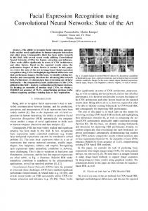
Figure 3. Visual comparisons between TV-L1 (FlowFields) with the motion estimates produced by MotionNet using TV-L1 (FlowFields) as proxy ground truth. The frame pairs are the same as in Figure 2.

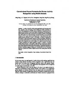
Figure 2. Visual comparisons of TV-L1 and our proposed MotionNet. Left: motion along x-axis. Right: motion along y-axis. MotionNet produces noisier motion estimates than TV-L1 in regions which are highly saturated or have dynamic textures. From top to bottom: Nunchunks, BeardShaving, Skijet and SkyDiving.

Method Stacked Temporal Stream (a) Hidden Two-Stream Networks (a)

No Proxy (%) 83.76 87.50

TV-L1 (%) 80.99 85.63

FlowFields (%) 79.82 85.40

Table 4. Incorporating extra proxy guidance does not help MotionNet generate better motion estimates for action recognition (UCF101 split1).

that the gap between model (c) and model (a)/(b) widens. The reason may be because that, without the regularization of unsupervised loss, the networks start to learn some appearance information. Hence they become less complementary to the spatial CNNs. Also, we can see that our models achieve very similar accuracy to the original two-stream CNNs. Among the two representative works we show, TwoStream CNNs [24] is the earliest two-stream work and Very Deep Two-Stream CNNs [32] is the one we improve upon. Therefore, Very Deep Two-Stream CNNs [32] are the most comparable ones. We can see that our approach is about 1% worse than Very Deep Two-Stream CNNs [32] in terms of accuracy but about 10x faster in terms of speed.

between the deconvolutions in the expanding part of MotionNet. This strategy is designed to smooth the motion estimation [18]. As can be seen in Table 3, removing extra convolutions brings a significant performance drop from 82.71% to 81.25%. Fourth, we examine the advantage of incorporating the smoothness objective. Without the smoothness loss, we obtain a much worse result of 80.14%. This result shows that our real-world data is very noisy. Adding smoothness regularization helps to generate smoother flow fields by suppressing the noise. This suppression is important for the following temporal stream CNNs to learn better motion representations for action recognition. Finally, we explore a configuration that does not employ any of these practices. As expected, the performance is the worst, which is 4.94% lower than our full MotionNet. Limitations of MotionNet Though our MotionNet outperforms other end-to-end methods[2, 9, 37] for action recognition, we are still far from exploiting its full potentials and perform 1% worse than traditional the optical flow estimation method (TV-L1)[36]. Here, we conduct a case by case comparison between MotionNet and TV-L1 algorithm, hoping to find where we could further improve our motion estimation. As we can see in Figure 2, MotionNet often produces noisier motion estimates than TV-L1. In particular, MotionNet has difficulties in regions which are highly saturated or have dynamic textures, for example, water, sky, and mirror. This difficulty is because the brightness constant assumption does not hold. For instance, in the second row of Figure 2, the true motion is shaving a beard, which is better outlined in the TV-L1 estimates. But due to the brightness

4.4. Discussion Ablation studies for MotionNet Because of our specifically designed objective functions and operators, our proposed MotionNet can produce high quality motion estimation, which helps us to get promising action recognition accuracy. In this section, we run an ablation study to understand the contributions of these components. The results are shown in Table 3. First, we examine the necessity of using a network structure focusing on small displacement motions. We keep other implementations the same, but use a larger kernel size and stride in the beginning of the network. The accuracy drops from 82.71% to 82.22%. This drop shows that using smaller kernels with a deeper network indeed help to detect small motions and improve our performance. Second, we examine the importance of adding SSIM loss. Without SSIM, the action recognition accuracy drops to 81.58% from 82.71%. This more than 1% performance drop shows that it is important to focus on discovering the structures of frame pairs. Similar observations can be found in [8] for unsupervised depth estimation. Third, we examine the effect of removing convolutions 7

Method Kantorov and Laptev [13] Tran et al. [27] Zhang et al. [37] Ng et al. [19] Diba et al. [5] Ours Simonyan and Zisserman [24] Bilen et al. [3] Wang et al. [32] Wang et al. [34] Zhu et al. [39] Wang et al. [33] Qiu et al. [22] Lan et al. [17] Diba et al. [6]

change of the mirror, MotionNet mistakenly estimates motion on the upper left corner as well. Taking the third row in Figure 2 as another example. TV-L1 can produce smooth flow fields of the moving jet ski. However, the flickering effect on the water surface makes it challenging for MotionNet to understand what is the real motion. Overall, it seems that MotionNet is more sensitive than TV-L1 in those areas where the brightness constant assumption does not hold. This phenomenon is mostly because MotionNet uses a global approach while TV-L1 uses a local approach. This phenomenon is also a potential reason that smaller kernels give us better performance. We will explore how to reduce the influence of global impact in the future. Will extra guidance help? Supervised optical flow learning methods [19, 38, 28, 5] showed that using optical flow from traditional methods (we called them proxy ground truths) can help CNNs to learn to predict motions. Given the limitations of MotionNet, we hope to correct those failure cases by using the predictions of robust flow estimators like TV-L1 as our proxy ground truth. Therefore, we investigate whether we can learn better motion estimation if we use proxy ground truth to guide the training of our MotionNet. We explore both TV-L1 [36] and FlowFields [2]. To our knowledge, TV-L1 is one of the mostly widely used and best performing flows for action recognition, and FlowFields is one of the most accurate flow estimators in the optical flow area 1 . The results are shown in Table 4. As can be seen, adding proxy guidance hurts performance. The action recognition accuracy drops about 2% when using TVL1 as proxy and 3% when using FlowFields. This result is counter-intuitive because FlowFields is often much better than TV-L1 for optical flow estimation tasks [2]. We show some qualitative results in Figure 3 to help us understand the reason behind this performance drop. As we can see, FlowFields generates much noisier optical flow than TV-L1 in real-world datasets. This noise is probably because FlowFields is designed to estimate large displacement motions, which happens a lot in synthetic datasets but much less often in real-world datasets. This result again demonstrates that EPE is not be an appropriate metric for evaluating motion estimates for action recognition tasks. In addition, as we can see in Figure 3, after incorporating proxy guidance, the motion estimates are much noisier and missing some motion boundaries. This noise could be the reason for the performance drop.

UCF101(%) − 85.2 86.4 70.0 90.2 90.3 88.0 89.1 91.4 92.4 93.0 94.2 95.2 95.3 95.6

HMDB51(%) 46.7 − − 42.6 − 58.9 59.4 65.2 62.0 68.2 69.4 − 75.0 71.1

Table 5. Comparison to state-of-the-art. Mean classification accuracy on UCF101 and HMDB51 over three splits.

section) and sub real-time (bottom section)2 . Note that although we list several most recent approaches here for comparison purposes, most of them are not directly comparable to our results due to the use of different network structures and improvement strategies. Among them, the most comparable one is Wang et al. [32], from which we build our approach. As can be seen, our method achieves similar accuracy to Wang et al. [32] and is much faster in inference. Diba et al. [5] can also have real-time performance and get similar accuracy as ours. This high accuracy is mostly because they train spatial and temporal stream together, which can be used in our method. Without joint training, their initial model has an accuracy of 85.2. Other slower methods achieve better performance than us for different reasons that have little to do with generating better optical flow. They either address part of the false label assignment problems, use a different and better encoding networks, or fuse the results from handcrafted features. For example, Wang et al. [33] use an inception network. Lan et al. [17] and Qiu et al. [22] use global pooling and fuse the results from IDTs. All these strategies can also be used by our models to improve the overall accuracy. For example, we can simply replace our network for encoding optical flow in [32] with the one in [33] to get better accuracy. Besides, all of these methods take TV-L1 flows as the inputs to their temporal stream CNNs. These computationally heavy inputs prevent them from being applied to largescale video datasets like Sports-1M [14] and YouTube-8M [1]. On the contrary, we can use those unlimited unlabeled videos to learn better MotionNet.

4.5. Comparison to State-of-the-Art

5. Conclusion

In this section, we compare our proposed method to recent state-of-the-art approaches as shown in Table 5. We divided the approaches into two categories, real-time (top

We have proposed a new framework called hidden twostream networks to recognize human actions in video. It addresses the problem that current CNN architectures have

1 For

2 In

FlowFields, we use the binary kindly provided by authors in [2].

8

general, the real-time requirement is 25 fps.

difficulty in capturing the temporal relationships among video frames. Differing from the current common practices of using traditional local optical flow estimation methods to pre-compute the motion information for CNNs, we use an unsupervised pre-training approach. Our motion estimation network (MotionNet) is computationally efficient and end-to-end trainable. Experimental results on UCF101 and HMDB51 show that our method is 10x faster than the traditional methods while maintaining similar accuracies. In the future, we would like to improve our hidden twostream networks in two directions. First, we improve our optical flow prediction by addressing the problems we have found. For example, we found that smoothness loss has a huge impact on the quality of the motion estimates for action recognition. Therefore, we will explore other welldesigned smoothness terms like edge aware loss [8] or scale invariant gradient loss [29] to further improve our accuracy. Second, we would like to improve other good practices that improve the overall performance of the networks. For example, we would also do joint training of spatial stream CNNs and stacked temporal stream CNNs. Also, it would be interesting to see how addressing false label assignment problem can help to improve our overall performance.

[10] M. Jaderberg, K. Simonyan, A. Zisserman, and K. Kavukcuoglu. Spatial Transformer Network. In NIPS, 2015. [11] S. Ji, W. Xu, M. Yang, and K. Yu. 3D Convolutional Neural Networks for Human Action Recognition. TPAMI, 2012. [12] Y. Jia, E. Shelhamer, J. Donahue, S. Karayev, J. Long, R. Girshick, S. Guadarrama, and T. Darrell. Caffe: Convolutional Architecture for Fast Feature Embedding. arXiv preprint arXiv:1408.5093, 2014. [13] V. Kantorov and I. Laptev. Efficient feature extraction, encoding and classification for action recognition. In CVPR, 2014. [14] A. Karpathy, G. Toderici, S. Shetty, T. Leung, R. Sukthankar, and L. Fei-Fei. Large-scale Video Classification with Convolutional Neural Networks. In CVPR, 2014. [15] H. Kuehne, H. Jhuang, E. Garrote, T. Poggio, and T. Serre. HMDB: A Large Video Database for Human Motion Recognition. In ICCV, 2011. [16] Z. Lan, M. Lin, X. Li, A. G. Hauptmann, and B. Raj. Beyond Gaussian Pyramid: Multi-skip Feature Stacking for Action Recognition. In CVPR, 2015. [17] Z. Lan, Y. Zhu, and A. G. Hauptmann. Deep Local Video Feature for Action Recognition. arXiv preprint arXiv:1701.07368, 2017. [18] N. Mayer, E. Ilg, P. Husser, P. Fischer, D. Cremers, A. Dosovitskiy, and T. Brox. A Large Dataset to Train Convolutional Networks for Disparity, Optical Flow, and Scene Flow Estimation. In CVPR, 2016. [19] J. Y.-H. Ng, J. Choi, J. Neumann, and L. S. Davis. ActionFlowNet: Learning Motion Representation for Action Recognition. arXiv preprint arXiv:1612.03052, 2016. [20] J. Y.-H. Ng, M. Hausknecht, S. Vijayanarasimhan, O. Vinyals, R. Monga, and G. Toderici. Beyond Short Snippets: Deep Networks for Video Classification. In CVPR, 2015. [21] X. Peng, C. Zou, Y. Qiao, and Q. Peng. Action Recognition with Stacked Fisher Vectors. In ECCV, 2014. [22] Z. Qiu, T. Yao, and T. Mei. Deep Quantization: Encoding Convolutional Activations with Deep Generative Model. arXiv preprint arXiv:1611.09502, 2016. [23] N. Sedaghat. Next-Flow: Hybrid Multi-Tasking with NextFrame Prediction to Boost Optical-Flow Estimation in the Wild. arXiv preprint arXiv:1612.03777, 2016. [24] K. Simonyan and A. Zisserman. Two-Stream Convolutional Networks for Action Recognition in Videos. NIPS, 2014. [25] K. Simonyan and A. Zisserman. Very Deep Convolutional Networks for Large-Scale Image Recognition. In ICLR, 2015. [26] K. Soomro, A. R. Zamir, and M. Shah. UCF101: A Dataset of 101 Human Action Classes From Videos in The Wild. In CRCV-TR-12-01, 2012. [27] D. Tran, L. Bourdev, R. Fergus, L. Torresani, and M. Paluri. Learning Spatiotemporal Features with 3D Convolutional Networks. In ICCV, 2015. [28] D. Tran, L. Bourdev, R. Fergus, L. Torresani, and M. Paluri. Deep End2End Voxel2Voxel Prediction. In CVPRW, 2016.

References [1] S. Abu-El-Haija, N. Kothari, J. Lee, P. Natsev, G. Toderici, B. Varadarajan, and S. Vijayanarasimhan. YouTube-8M: A Large-Scale Video Classification Benchmark. arXiv preprint arXiv:1609.08675, 2016. [2] C. Bailer, B. Taetz, and D. Stricker. Flow Fields: Dense Correspondence Fields for Highly Accurate Large Displacement Optical Flow Estimation. In ICCV, 2015. [3] H. Bilen, B. Fernando, E. Gavves, A. Vedaldi, and S. Gould. Dynamic Image Networks for Action Recognition. In CVPR, 2016. [4] J. Deng, W. Dong, R. Socher, L.-J. Li, K. Li, and L. Fei-Fei. ImageNet: A Large-Scale Hierarchical Image Database. In CVPR, 2009. [5] A. Diba, A. M. Pazandeh, and L. V. Gool. Efficient TwoStream Motion and Appearance 3D CNNs for Video Classification. arXiv preprint arXiv:1608.08851, 2016. [6] A. Diba, V. Sharma, and L. V. Gool. Deep Temporal Linear Encoding Networks. arXiv preprint arXiv:1611.06678, 2016. [7] P. Fischer, A. Dosovitskiy, E. Ilg, P. Husser, C. Hazrba, V. Golkov, P. van der Smagt, D. Cremers, and T. Brox. FlowNet: Learning Optical Flow with Convolutional Networks. In ICCV, 2015. [8] C. Godard, O. M. Aodha, and G. J. Brostow. Unsupervised Monocular Depth Estimation with Left-Right Consistency. In CVPR, 2017. [9] E. Ilg, N. Mayer, T. Saikia, M. Keuper, A. Dosovitskiy, and T. Brox. FlowNet 2.0: Evolution of Optical Flow Estimation with Deep Networks. arXiv preprint arXiv:1612.01925, 2016.

9

[29] B. Ummenhofer, H. Zhou, J. Uhrig, N. Mayer, E. Ilg, A. Dosovitskiy, and T. Brox. DeMoN: Depth and Motion Network for Learning Monocular Stereo. arXiv preprint arXiv:1612.02401, 2016. [30] G. Varol, I. Laptev, and C. Schmid. Long-term Temporal Convolutions for Action Recognition. arXiv preprint arXiv:1604.04494, 2016. [31] H. Wang and C. Schmid. Action Recognition with Improved Trajectories. In ICCV, 2013. [32] L. Wang, Y. Xiong, Z. Wang, and Y. Qiao. Towards Good Practices for Very Deep Two-Stream ConvNets. arXiv preprint arXiv:1507.02159, 2015. [33] L. Wang, Y. Xiong, Z. Wang, Y. Qiao, D. Lin, X. Tang, and L. V. Gool. Temporal Segment Networks: Towards Good Practices for Deep Action Recognition. In ECCV, 2016. [34] X. Wang, A. Farhadi, and A. Gupta. Actions˜ Transformations. In CVPR, 2016. [35] J. J. Yu, A. W. Harley, and K. G. Derpanis. Back to Basics: Unsupervised Learning of Optical Flow via Brightness Constancy and Motion Smoothness. arXiv preprint arXiv:1608.05842, 2016. [36] C. Zach, T. Pock, and H. Bischof. A Duality Based Approach for Realtime TV-L1 Optical Flow. In 29th DAGM conference on Pattern recognition, 2014. [37] B. Zhang, L. Wang, Z. Wang, Y. Qiao, and H. Wang. Real-time Action Recognition with Enhanced Motion Vector CNNs. In CVPR, 2016. [38] Y. Zhu, Z. Lan, S. Newsam, and A. G. Hauptmann. Guided Optical Flow Learning. arXiv preprint arXiv:1702.022952, 2016. [39] Y. Zhu and S. Newsam. Depth2Action: Exploring Embedded Depth for Large-Scale Action Recognition. In ECCVW, 2016.

10