Temporal Convolutional Networks for Action Segmentation and ...

Temporal Convolutional Networks for Action Segmentation and Detection Michael D. Flynn Ren´e Vidal Austin Reiter Gregory D. Hager Johns Hopkins University {clea1@, mflynn@, rvidal@cis., areiter@cs., hager@cs.}jhu.edu

arXiv:1611.05267v1 [cs.CV] 16 Nov 2016

Colin Lea

Abstract The ability to identify and temporally segment finegrained human actions throughout a video is crucial for robotics, surveillance, education, and beyond. Typical approaches decouple this problem by first extracting local spatiotemporal features from video frames and then feeding them into a temporal classifier that captures high-level temporal patterns. We introduce a new class of temporal models, which we call Temporal Convolutional Networks (TCNs), that use a hierarchy of temporal convolutions to perform fine-grained action segmentation or detection. Our Encoder-Decoder TCN uses pooling and upsampling to efficiently capture long-range temporal patterns whereas our Dilated TCN uses dilated convolutions. We show that TCNs are capable of capturing action compositions, segment durations, and long-range dependencies, and are over a magnitude faster to train than competing LSTM-based Recurrent Neural Networks. We apply these models to three challenging fine-grained datasets and show large improvements over the state of the art.

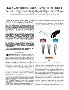
Figure 1. Our Encoder-Decoder Temporal Convolutional Network (ED-TCN) hierarchically models actions using temporal convolutions, pooling, and upsampling.

ically do not capture long-range temporal patterns; segmental models [24, 15, 23], which capture within-segment properties but assume conditional independence, thereby ignoring long-range latent dependencies; and recurrent models [27, 9], which can capture latent temporal patterns but are difficult to interpret, have been found empirically to have a limited span of attention [27], and are hard to correctly train [21]. In this paper, we discuss a class of time-series models, which we call Temporal Convolutional Networks (TCNs), that overcome the previous shortcomings by capturing longrange patterns using a hierarchy of temporal convolutional filters. We present two types of TCNs: First, our EncoderDecoder TCN (ED-TCN) only uses a hierarchy of temporal convolutions, pooling, and upsampling but can efficiently capture long-range temporal patterns. The ED-TCN has a relatively small number of layers (e.g., 3 in the encoder) but each layer contains a set of long convolutional filters. Second, a Dilated TCN uses dilated convolutions instead of

1. Introduction Action segmentation is crucial for applications ranging from collaborative robotics to analysis of activities of daily living. Given a video, the goal is to simultaneously segment every action in time and classify each constituent segment. In the literature, this task goes by either action segmentation or detection. We focus on modeling situated activities – such as in a kitchen or surveillance setup – which are composed of dozens of actions over a period of many minutes. These actions, such as cutting a tomato versus peeling a cucumber, are often only subtly different from one another. Current approaches decouple this task into extracting low-level spatiotemporal features and applying high-level temporal classifiers. While there has been extensive work on the former, recent temporal models have been limited to sliding window action detectors [25, 27, 20], which typ1

pooling and upsampling and adds skip connections between layers. This is an adaptation of the recent WaveNet [33] model, which shares similarities to our ED-TCN but was developed for speech processing tasks. The Dilated TCN has more layers, but each uses dilated filters that only operate on a small number of time steps. Empirically, we find both TCNs are capable of capturing features of segmental models, such as action durations and pairwise transitions between segments, as well as long-range temporal patterns similar to recurrent models. These models tend to outperform our Bidirectional LSTM (Bi-LSTM) [5] baseline and are over a magnitude faster to train. The ED-TCN in particular produces many fewer over-segmentation errors than other models. In the literature, our task goes by the name action segmentation [7, 8, 6, 14, 28, 15, 9] or action detection [27, 19, 20, 24]. Despite effectively being the same problem, the temporal methods in segmentation papers tends to differ from detection papers, as do the metrics by which they are evaluated. In this paper, we evaluate on datasets targeted at both tasks and propose a segmental F1 score, which we qualitatively find is more applicable to real-world concerns for both segmentation and detection than common metrics. We use MERL Shopping which was designed for action detection, Georgia Tech Egocentric Activities which was designed for action segmentation, and 50 Salads which has been used for both. Code for our models and metrics, as well as dataset features and predictions,1 will be released upon acceptance.

2. Related Work Action segmentation methods predict what action is occurring at every frame in a video and detection methods output a sparse set action segments, where a segment is defined by a start time, end time, and class label. It is possible to convert between a given segmentation and set of detections by simply adding or removing null/background segments. Action Detection: Many fine-grained detection papers use sliding window-based detection methods on spatial or spatiotemporal features. Rohrbach et al. [25] used Dense Trajectories [36] and human pose features on the MPII Cooking dataset. At each frame they evaluated a sliding SVM for many candidate segment lengths and performed nonmaximal suppression to find a small set of action predictions. Ni et al. [20] used an object-centric feature representation, which iteratively parses object locations and spatial configurations, and applied it to the MPII Cooking and ICPR 2012 Kitchen datasets. Their approach used Dense Trajectory features as input into a sliding-window detection method with segment intervals of 30, 60, and 90 frames. 1 The release of the MERL Shopping features depends on the permission of the original authors. All other features will be available.

Singh et al. [27] improved upon this by feeding per-frame CNN features into an LSTM model and applying a method analogous to non-maximal suppression to the LSTM output. We use Singh’s proposed dataset, MERL Shopping, and show our approach outperforms their LSTM-based detection model. Recently, Richard et al. [24] introduced a segmental approach that incorporates a language model, which captures pairwise transitions between segments, and a duration model, which ensures that segments are of an appropriate length. In the experiments we show that our model is capable of capturing both of these components. Some of these datasets, including MPII Cooking, have been used for classification (e.g., [3, 38]), however, this task assumes the boundaries of each segment are known. Action Segmentation: Segmentation papers tend to use temporal models that capture high-level patterns, for example RNNs or Conditional Random Fields (CRFs). The line of work by Fathi et al. [8, 7, 6] used a segmental model that captured object states at the start and end of each action (e.g., the appearance of bread before and after spreading jam). They applied their work to the Georgia Tech Egocentric Activities (GTEA) dataset, which we use in our experiments. Singh et al. [28] used an ensemble of CNNs to extract egocentric-specific features on the GTEA dataset but did not use a high-level temporal model. Lea et al. [15] introduced a spatiotemporal CNN with a constrained segmental model which they applied to 50 Salads. Their model reduced the number of action over-segmentation errors by constraining the maximum number of candidate segments. We show our TCNs produce even fewer over-segmentation errors. Kuehne et al. [13, 14] modeled actions using Hidden Markov Models on Dense Trajectory features, which they applied with a high-level grammar to 50 Salads. Other work has looked at semi-supervised methods for action segmentation, such as Huang et al. [9], which reduces the number of required annotations and improves performance when used with RNN-based models. It is possible that their approach could be used with TCNs for improved performance. Large-scale Recognition: There has been substantial work on spatiotemporal models for large scale video classification and detection [30, 10, 11, 26, 32, 22, 18]. These focus on capturing object- and scene-level information from short sequences of images and thus are considered orthogonal to our work, which focuses on capturing longer-range temporal information. The input into our model could be the output of a spatiotemporal CNN. Other related models: There are parallels between TCNs and recent work on semantic segmentation, which uses Fully Convolutional CNNs to compute a per-pixel object labeling of a given image. The Encoder-Decoder TCN is most similar to SegNet [2] whereas the Dilated TCN is most similar to the Multi-Scale Context model [37]. TCNs are also related to Time-Delay Neural Networks (TDNNs), which

were introduced by Waibel et al. [35] in the early 1990s. TDNNs apply a hierarchy of temporal convolutions across the input but do not use pooling, skip connections, newer activations (e.g., Rectified Linear Units), or other features of our TCNs.

3. Temporal Convolutional Networks In this section we define two TCNs, each of which have the following properties: (1) computations are performed layer-wise, meaning every time-step is updated simultaneously, instead of updating sequentially per-frame (2) convolutions are computed across time, and (3) predictions at each frame are a function of a fixed-length period of time, which is referred to as the receptive field. Our ED-TCN uses an encoder-decoder architecture with temporal convolutions and the Dilated TCN, which is adapted from the WaveNet model, uses a deep series of dilated convolutions. The input to a TCN will be a set of video features, such as those output from a spatial or spatiotemporal CNN, for each frame of a given video. Let Xt ∈ RF0 be the input feature vector of length F0 for time step t for 1 ≤ t ≤ T . Note that the number of time steps T may vary for each video sequence. The action label for each frame is given by vector Yt ∈ {0, 1}C , where C is the number of classes, such that the true class is 1 and all others are 0.

3.1. Encoder-Decoder TCN Our encoder-decoder framework is depicted in Figure 1. The encoder consists of L layers denotes by E (l) ∈ RFl ×Tl where Fl is the number of convolutional filters in a the lth layer and Tl is the number of corresponding time steps. Each layer consists of temporal convolutions, a non-linear activation function, and max pooling across time. We define the collection of filters in each layer as W = (i) l {W (i) }F ∈ Rd×Fl−1 with a corresponding bias i=1 for W Fl vector b ∈ R . Given the signal from the previous layer, E (l−1) , we compute activations E (l) with E (l) = f (W ∗ E (l−1) + b)

(1)

where f (·) is the activation function and ∗ is the convolution operator. We compare activation functions in Section 4.4 and find normalized Rectified Linear Units perform best. After each activation function, we max pool with width 2 across time such that Tl = 12 Tl−1 . Pooling enables us to efficiently compute activations over long temporal windows. Our decoder is similar to the encoder, except that upsampling is used instead of pooling and the order of the operations is now upsample, convolve, and apply the activation function. Upsampling is performed by simply repeating each entry twice. The convolutional filters in the decoder distribute the activations from the condensed layers in the middle to the action predictions at the top. Experimentally,

Figure 2. The Dilated TCN model uses a deep stack of dilated convolutions to capture long-range temporal patterns.

these convolutions provide a large improvement in performance and appear to capture pairwise transitions between actions. Each decoder layer is denoted by D(l) ∈ RFl ×Tl for l ∈ {L, . . . , 1}. Note that these are indexed in reverse order compared to the encoder, so the filter count in the first encoder layer is the same as in the last decoder layer. The probability that frame t corresponds each of the C action classes is given by vector Yˆt ∈ [0, 1]C using weight matrix U ∈ RC×F1 and bias c ∈ RC , such that (1) Yˆt = softmax(U Dt + c).

(2)

We explored other mechanisms, such as skip connections between layers, different patterns of convolutions, and other normalization schemes, however, the proposed model outperformed these alternatives and is arguably simpler. Implementation details are described in Section 3.3. Receptive Field: The prediction at each frame is a function of a fixed-length period of time, which is given by the r(d, L) = d(2L − 1) + 1 for L layers and duration d.

3.2. Dilated TCN We adapt the WaveNet [33] model, which was designed for speech synthesis, to the task of action segmentation. In their work, the predicted output, Yt , denoted which audio sample should come next given the audio from frames 1 to t. In our case Yt is the current action given the video features up to t. As shown in Figure 2, we define a series of blocks, each of which contains a sequence of L convolutional layers. The activations in the l-th layer and j-th block are given by S (j,l) ∈ RFw ×T . Note that each layer has the same number of filters Fw . This enables us to combine activations from different layers later. Each layer consists a set

of dilated convolutions with rate parameter s, a non-linear activation f (·), and a residual connection than combines the layer’s input and the convolution signal. Convolutions are only applied over two time steps, t and t − s, so we write out the full equations to be specific. The filters are parameterized by W = {W (1) , W (2) } with W (i) ∈ RFw ×Fw and (j,l) bias vector b ∈ RFw . Let Sˆt be the result of the dilated (j,l) convolution at time t and St be the result after adding the residual connection such that (j,l) (j,l−1) (j,l−1) Sˆt = f (W (1) St−s + W (2) St + b) (j,l)

St

(j,l−1)

= St

(j,l) + V Sˆt + e.

(3) (4)

Let V ∈ RFw ×Fw and e ∈ RFw be a set of weights and biases for the residual. Note that parameters {W, b, V, e} are separate for each layer. The dilation rate increases for consecutive layers within a block such that sl = 2l . This enables us to increase the receptive field by a substantial amount without drastically increasing the number of parameters. The output of each block is summed using a set of skip connections with Z (0) ∈ RT ×Fw such that (0)

Zt

B X (j,L) = ReLU ( St ).

(5)

j=1 (1)

(0)

There is a set of latent states Zt = ReLU (Vr Zt +er ) for weight matrix Vr ∈ RFw ×Fw and bias er . The predictions for each time t are given by (1) Yˆt = sof tmax(U Zt + c)

(6)

for weight matrix U ∈ RC×Fw and bias c ∈ RC . Receptive Field: The filters in each Dilated TCN layer are smaller than in ED-TCN, so in order to get an equal-sized receptive field it needs more layers or blocks. The expression for its receptive field is r(B, L) = B ∗ 2L for number of blocks B and number of layers per block L.

3.3. Implementation details Parameters of both TCNs are learned using the categorical cross entropy loss with Stochastic Gradient Descent and ADAM [12] step updates. Using dropout on full convolutional filters [31], as opposed to individual weights, improves performance and produces smoother looking weights. For ED-TCN, each of the L layers has Fl = 96 + 32 ∗ l filters. For the Dilated TCN we find that performance does not depend heavily on the number of filters for each convolutional layer, so we set Fw = 128. We perform ablative analysis with various number of layers and filter durations in the experiments. All models were implemented using Keras [4] and TensorFlow [1].

3.4. Causal versus Acausal We perform causal and acausal experiments. Causal means that the prediction at time t is only a function of data from times 1 to t, which is important for applications in robotics. Acausal means that the predictions may be a function of data at any time step in the sequence. For the causal case in ED-TCN, for at each time step t and filter length d, we convolve from Xt−d to Xt . In the acausal case we convolve from Xt− d to Xt+ d . 2 2 For the acausal Dilated TCN, we modify Eqn 3 such that each layer now operates over one previous step, the current step, and one future step: (j,l) (j,l−1) (j,l−1) Sˆt = f (W (1) St−s + W (2) St (j,l−1)

+ W (3) St+s

+ b)

(7)

where now W = {W (1) , W (2) , W (3) }.

4. Evaluation & Discussion We start by performing synthetic experiments that highlight the ability of our TCNs to capture high-level temporal patterns. We then perform quantitative experiments on three challenging datasets and ablative analysis to measure the impact of hyper-parameters such as filter duration.

4.1. Metrics Papers addressing action segmentation tend to use different metrics than those on action detection. We evaluate using metrics from both communities and introduce a segmental F1 score, which is applicable to both tasks. Segmentation metrics: Action segmentation papers tend use to frame-wise metrics, such as accuracy, precision, and recall [29, 13]. Some work on 50 Salads also uses segmental metrics [15, 16], in the form of a segmental edit distance, which is useful because it penalizes predictions that are outof-order and for over-segmentation errors. We evaluate all methods using frame-wise accuracy. One drawback of frame-wise metrics is that models achieving similar accuracy may have large qualitative differences, as visualized later. For example, a model may achieve high accuracy but produce numerous oversegmentation errors. It is important to avoid these errors for human-robot interaction and video summarization. Detection metrics: Action detection papers tend to use segment-wise metrics such as mean Average Precision with midpoint hit criterion (mAP@mid) [25, 27] or mAP with a intersection over union (IoU) overlap criterion (mAP@k) [24]. mAP@k is computed my comparing the overlap score for each segment with respect to the ground truth action of the same class. If an IoU score is above a k it is considered a true positive otherwise threshold τ = 100

it is a false positive. Average precision is computed for each class and the results are averaged. mAP@mid is similar except the criterion for a true positive is whether or not the midpoint (mean time) is within the start and stop time of the corresponding correct action. mAP is a useful metric for information retrieval tasks like video search, however for many fine-grained action detection applications, such as robotics or video surveillance, we find that results are not indicative of real-world performance. The key issue is that mAP is very sensitive to a confidence score assigned to each segment prediction. These confidences are often simply the mean or maximum class score within the frames corresponding to a predicted segment. By computing these confidences in subtly different ways you obtain wildly different results. On MERL Shopping, the mAP@mid scores for Singh et al. [27] jump from 50.9 using the mean prediction score over an interval to 69.8 using the maximum score over that same interval. F1@k: We propose a segmental F1 score which is applicable to both segmentation and detection tasks and has the following properties: (1) it penalizes over-segmentation errors, (2) it does not penalize for minor temporal shifts between the predictions and ground truth, which may have been caused by annotator variability, and (3) scores are dependent on the number actions and not on the duration of each action instance. This metric is similar to mAP with IoU thresholds except that it does not require a confidence for each prediction. Qualitatively, we find these numbers are better at indicating the caliber of a given segmentation. We compute whether or not each predicted action segment is a true or false positive by comparing its IoU with respect to the corresponding ground truth using threshold τ . As with mAP detection scores, if there is more than one correct detection within the span of a single true action then only one is marked as a true positive and all others are false positives. We compute precision and recall for true positives, false positives, and false negatives summed over all prec∗recall . classes and compute F 1 = 2 prec+recall We attempted to obtain action predictions from the original authors on all datasets to compare across multiple metrics. We received them for 50 Salads and MERL Shopping.

4.2. Synthetic Experiments We claim TCNs are capable of capturing complex temporal patterns, such as action compositions, action durations, and long-range temporal dependencies. We show these abilities with two synthetic experiments. For each, we generate toy features X and corresponding labels Y for 50 training sequences and 10 test sequences of length T = 150. The duration of each action of a given class is fixed and action segments are sampled randomly. An example for the composition experiment is shown in Figure 3. Both TCNs are acausal and have a receptive field of length 16.

Figure 3. Synthetic Experiment #1: (top) True action labels for a given sequence (bottom) The 3 dimensional features for that sequence. White is −1 and gray is +1. Subctions A1, A2, and A3 (dark blue, light blue and green) all have to the same feature values, which differ from B (orange) and C (red).

Shift ED-TCN Dilated TCN Bi-LSTM

s=0 100 100 100

s=5 97.9 92.7 72.3

s=10 89.5 87.0 60.2

s=15 74.1 69.6 54.7

s=20 57.1 61.5 38.5

Table 1. Synthetic experiment #2: F1@10 when shifting the input features in time with respect to the true labels. Column shows performance when shifting the data s frames from the corresponding labels. Each TCN receptive field is 16 frames.

Action Compositions: By definition, an activity is composed of a sequence of actions. Typically there is a dependency between consecutive actions (e.g., action B likely comes after A). CRFs capture this using a pairwise transition model over class labels and RNNs capture it using LSTM across latent states. We show that TCNs can capture action compositions, despite not explicitly conditioning the activations at time t on previous time steps within that layer. In this experiment, we generated sequences using a Markov model with three high-level actions A, B, and C with subactions A1 , A2 , and A3 , as shown in Figure 3. A always consists of subactions A1 (dark blue), A2 (light blue), then A3 (green), after which it is transitions to B or C. For simplicity, Xt ∈ R3 corresponds to the high-level action Yt such that the true class is +1 and others are −1. The feature vectors corresponding to subactions A1−A3 are all the same, thus a simple frame-based classifier would not be able to differentiate them. The TCNs, given their long receptive fields, segment the actions perfectly. This suggests that our TCNs are capable of capturing action compositions. Recall each action class had a different segment duration, and we correctly labeled all frames, which suggests TCNs can capture duration properties for each class. Long-range temporal dependencies: For many actions it is important to consider information from seconds or even minutes in the past. For example, in the cooking scenario, when a user cuts a tomato, they tend to occlude the tomato with their hands, which makes it difficult to identify which object is being cut. It would be advantageous to recognize that the tomato is on the cutting board before the user starts the cutting action. In this experiment, we show TCNs are capable of learning these long-range temporal patterns by

adding a phase delay to the features. Specifically, for both ˆ as X ˆ t = Xt−s for all training and test features we define X t. Thus, there is a delay of s frames between the labels and the corresponding features. Results using F1@10 are shown in 4.2. For comparison we show the TCNs as well as Bi-LSTM. As expected, with no delay (s = 0) all models achieve perfect prediction. For short delays (s = 5), TCNs correctly detect all actions except the first and last of a sequence. As the delay increases, ED-TCN and Dilated TCN perform very well up to about half the length of the receptive field. The results for Bi-LSTM degrade at a much faster rate.

4.3. Datasets University of Dundee 50 Salads [29]: contains 50 sequences of users making a salad and has been used for both action segmentation and detection. While this is a multimodal dataset we only evaluate using the video data. Each video is 5-10 minutes in duration and contains around 30 instances of actions such as cut tomato or peel cucumber. We performed cross validation with 5 splits on a higher-level action granularity which includes 9 action classes such as add dressing, add oil, cut, mix ingredients, peel, and place, plus a background class. In [29] this was referred to as “eval.” We also evaluate on a mid-level action granularity with 17 action classes. The mid-level labels differentiates actions like cut tomato from cut cucumber whereas the higher-level combines these into a single class, cut. We use the spatial CNN features of Lea et al. [15] as input into our models. This is a simplified VGG-style model trained solely on 50 Salads. Data was downsampled to approximately 1 frame/second. MERL Shopping [27]: is an action detection dataset consisting of 106 surveillance-style videos in which users interact with items on store shelves. The camera viewpoint is fixed and only one user is present in each video. There are five actions plus a background class: reach to shelf, retract hand from shelf, hand in shelf, inspect product, inspect shelf. Actions are typically a few seconds long. We use the features from Singh et al. [27] as input. Singh’s model consists of four VGG-style spatial CNNs: one for RGB, one for optical flow, and ones for cropped versions of RGB and optical flow. We stack the four featuretypes for each frame and use Principal Components Analysis with 50 components to reduce the dimensionality. The train, validation, and test splits are the same as described in [27]. Data is sampled at 2.5 frames/second. Georgia Tech Egocentric Activities (GTEA) [8]: contains 28 videos of 7 kitchen activities such as making a sandwich and making coffee. The four subjects performed each activity once. The camera is mounted on the user’s head and is

50 Salads (higher) Spatial CNN [15] Dilated TCN ST-CNN [15] Bi-LSTM ED-TCN 50 Salads (mid) Spatial CNN [15] IDT+LM [24] Dilated TCN ST-CNN [15] Bi-LSTM ED-TCN

F1@{10, 25, 50} 35.0, 30.5, 22.7 55.8, 52.3, 44.3 61.7, 57.3, 47.2 72.2, 68.4, 57.8 76.5, 73.8, 64.5 F1@{10, 25, 50} 32.3, 27.1, 18.9 44.4, 38.9, 27.8 52.2, 47.6, 37.4 55.9, 49.6, 37.1 62.6, 58.3, 47.0 68.0, 63.9, 52.6

Edit 25.5 46.9 52.8 67.7 72.2 Edit 24.8 45.8 43.1 45.9 55.6 59.8

Acc 68.0 71.1 71.3 70.9 73.4 Acc 54.9 48.7 59.3 59.4 55.7 64.7

Table 2. Action segmentation results 50 salads. F1@k is our segmental F1 score, Edit is the Segmental edit score from [16], and Acc is frame-wise accuracy.

pointing towards their hands. On average there are about 19 (non-background) actions per video and videos are around a minute long. We use the 11 action classes defined in [6] and evaluate using leave one user out. Cross-validation is performed over users 1-3 as done by [28]. We use a frame rate of 3 frames per second. We were unable to obtain state of the art features from [28], so we trained spatial CNNs from scratch using code from [15], which was originally applied to 50 Salads. This is a simplified VGG-style network where the input for each frame is a pair of RGB and motion images. Optical flow is very noisy due to large amounts of video compression in this dataset, so we simply use difference images, such that for image It at frame t the motion image is the concatenation of [It−d − It , It+d − It , It−2d − It , It+2d − It ] for delay d = 0.5 seconds. These difference images can be viewed as a simple attention mechanism. We compare results from this spatial CNN, the spatiotemporal CNN from [15], EgoNet [28], and our TCNs.

4.4. Experimental Results To make the baselines more competitive, we apply Bidirectional LSTM (Bi-LSTM) [5] to 50 Salads and GTEA. We use 64 latent states per LSTM direction with the same loss and learning methods as previously described. The input to this model is the same as for the TCNs. Note that MERL Shopping already has this baseline. 50 Salads: Results on both action granularities are included in Table 4.4. All methods are evaluated in acausal mode. ED-TCN outperforms all other models on both granularities and on all metrics. We also compare against Richard et al. [24] who evaluated on the mid-level and reported using IoU mAP detection metrics. Their approach achieved 37.9 mAP@10 and 22.9 mAP@50. The ED-TCN achieves 64.9 mAP@10 and 42.3 mAP@50 and Dilated TCN achieves 53.3 mAP@10 and 29.2 mAP@50.

MERL (acausal) MSN Det [27] MSN Seg [27] Dilated TCN ED-TCN MERL (causal) MSN Det [27] Dilated TCN ED-TCN

F1@{10, 25, 50} 46.4, 42.6, 25.6 80.0, 78.3, 65.4 79.9, 78.0, 67.5 86.7, 85.1, 72.9 F1@{10, 25, 50} 72.7, 70.6, 56.5 82.1, 79.8, 64.0

mAP 81.9 69.8 75.6 74.4 mAP 77.6 72.2 64.2

Acc 64.6 76.3 76.4 79.0 Acc 73.0 74.1

Table 3. MERL Shopping results. Action segmentation results on the MERL Shopping dataset. Causal only uses features from previous time steps and acausal uses previous and future time steps. mAP refers to mean Average Precision with midpoint hit criterion.

GTEA EgoNet+TDD [28] Spatial CNN [15] ST-CNN [15] Dilated TCN Bi-LSTM ED-TCN

F1@{10,25,50} 41.8, 36.0, 25.1 58.7, 54.4, 41.9 58.8, 52.2, 42.2 66.5, 59.0, 43.6 72.2, 69.3, 56.0

Acc 64.4 54.1 60.6 58.3 55.5 64.0

Table 4. Action segmentation results on the Georgia Tech Egocentric Activities dataset. F1@k is our segmental F1 score and Acc is frame-wise accuracy.

Notice that ED-TCN, Dilated TCN, and ST-CNN all achieve similar frame-wise accuracy but very different F1@k and edit scores. ED-TCN tends to produce many fewer over-segmentations than competing methods. Figure 5 shows mid-level predictions for these models. Accuracy and F1 for each prediction is included for comparison. Many errors on this dataset are due to the extreme similarity between actions and subtle differences in object appearance. For example, our models confuse actions using the vinegar and olive oil bottles, which have a similar appearance. Similarly, we confuse some cutting actions (e.g., cut cucumber versus cut tomato) and placing actions (e.g., place cheese versus place lettuce). MERL Shopping: We compare against use two sets of predictions from Singh et al. [27], as shown in Table 4.4. The first, as reported in their paper, are a sparse set of action detections which are referred to as MSN Det. The second, obtained from the authors, are a set of dense (per-frame) action segmentations. The detections use activations from the dense segmentations with a non-maximal suppression detection algorithm to output a sparse set of segments. Their causal version uses LSTM on the dense activations and their acausal version uses Bidirectional LSTM. While Singh’s detections achieve very high midpoint mAP, the same predictions perform very poorly on the other metrics. As visualized in Figure 5 (right), the actions are very short and sparse. This is advantageous when optimizing for midpoint mAP, because performance only depends

Figure 4. Receptive field experiments (left) ED-TCN: varying layer count L and filter durations d (right) Dilated TCN: varying layer count L and number of blocks B.

on the midpoint of a given action, however, it it not effective if you require the start and stop time of an activity. Interesting, this method does worst in F1 even for low overlaps. As expected the acausal TCNs perform much better than the causal variants. This verifies that using future information is important for achieving best performance. In the causal and acausal results the Dilated TCN outperforms ED-TCN in midpoint mAP, however, the F1 scores are better for ED-TCN. This suggests the confidences for the Dilated TCN are more reliable than ED-TCN. Georgia Tech Egocentric Activities: Performance of the ED-TCN is on par with the ensemble approach of Singh et al. [28], which combines EgoNet features with TDD [17]. Recall that Singh’s approach does not incorporate a temporal model, so we expect that combining their features with our ED-TCN would improve performance. Unlike EgoNet and TDD, our approach uses simpler spatial CNN features which can be computed in real-time. Overall, in our experiments the Encoder-Decoder TCN outperformed all other models, including state of the art approaches for most datasets and our adaptation of the recent WaveNet model. The most important difference between these models is that ED-TCN uses fewer layers but has longer convolutional filters whereas the Dilated TCN has more layers but with shorter filters. The long filters in ED-TCN have a strong positive affect on F1 performance, in particular because they prevent over-segmentation issues. The Dilated TCN performs well on metrics like accuracy, but is less robust to over-segmentation. This is likely due to the short filter lengths in each layer. 4.4.1

Ablative Experiments

Ablative experiments were performed on 50 Salads (midlevel). Note that these were done with different hyperparameters and thus may not match previous results. Activation functions: We assess performance using the activation functions shown in Table 4.4.1. The Gated PixelCNN (GPC) activation [34], f (x) = tanh(x)

50 Salads

MERL Shopping

GTEA

Figure 5. (top) Example images from each dataset. (bottom) Action predictions for one sequence using the mid-level action set of 50 Salads (left) and on MERL Shopping (right). These timelines are “typical.” Performance is near the average performance across each dataset.

Activation ED-TCN Dilated TCN

Sigm. 37.3 42.5

ReLU 40.4 43.1

Tanh 48.1 41.0

GPC 52.7 40.5

NReLU 58.4 40.7

Table 5. Comparison of different activation functions used in each TCN. Results are computed on 50 Salads (mid-level) with F1@25.

sigmoid(x), was used for WaveNet and also achieves high performance on our tasks. We define the Normalized ReLU f (x) =

ReLU (x) , max(ReLU (x)) + 

(8)

for vector x and  = 1E -5 where the max is computed perframe. Normalized ReLU outperforms all others with EDTCN, whereas for Dilated TCN all functions are similar. Receptive fields: We compare performance with varying receptive field hyperparameters. Line in Figure 4 (left) show F1@25 for L from 1 to 5 and filter sizes d from 1 to 40 on ED-TCN. Lines in Figure 4 (right) correspond to block count B with layer count L from 1 to 6 for a Dilated TCN. Note, our GPU ran out of memory on ED-TCN after (L = 4,d = 25) and Dilated TCN after (B = 4,L = 5). The ED-TCN performs best with a receptive field of 44 frames (L = 2,d = 15) which corresponds to 52 seconds. The Dilated TCN performs best at 128 frames (B = 4,L = 5) and achieves similar performance at 96 frames (B = 3,L = 5).

Training time: It takes much less time to train a TCN than a Bi-LSTM. While the exact timings vary with the number of TCN layers and filter lengths, for one split of 50 Salads – using a Nvidia Titan X for 200 epochs – it takes about a minute to train the ED-TCN whereas and 30 minutes to train the Bi-LSTM. This speedup comes from the fact that activations within each TCN layer are all independent, and thus they can be performed in batch on a GPU. Activations in intermediate RNN layers depend on previous activations within that layer, so operations must be applied sequentially.

5. Conclusion We introduced Temporal Convolutional Networks, which use a hierarchy of convolutions to capture long-range temporal patterns. We showed on synthetic data that TCNs are capable of capturing complex patterns such as compositions, action durations, and are robust to time-delays. Our models outperformed strong baselines, including Bidirectional LSTM, and achieve state of the art performance on challenging datasets. We believe TCNs are a formidable alternative to RNNs and are worth further exploration. Acknowledgments: Thanks to Bharat Singh and the group at MERL for discussions on their dataset and for letting us use the spatiotemporal features as input into our model. We also thank Alexander Richard for his 50 Salads predictions.

References [1] M. Abadi, A. Agarwal, P. Barham, E. Brevdo, Z. Chen, C. Citro, G. S. Corrado, A. Davis, J. Dean, M. Devin, S. Ghemawat, I. Goodfellow, A. Harp, G. Irving, M. Isard, Y. Jia, R. Jozefowicz, L. Kaiser, M. Kudlur, J. Levenberg, D. Man´e, R. Monga, S. Moore, D. Murray, C. Olah, M. Schuster, J. Shlens, B. Steiner, I. Sutskever, K. Talwar, P. Tucker, V. Vanhoucke, V. Vasudevan, F. Vi´egas, O. Vinyals, P. Warden, M. Wattenberg, M. Wicke, Y. Yu, and X. Zheng. TensorFlow: Large-scale machine learning on heterogeneous systems, 2015. Software available from tensorflow.org. 4 [2] V. Badrinarayanan, A. Handa, and R. Cipolla. Segnet: A deep convolutional encoder-decoder architecture for robust semantic pixel-wise labelling. arXiv preprint arXiv:1505.07293, 2015. 2 [3] G. Cheron, I. Laptev, and C. Schmid. P-cnn: Pose-based cnn features for action recognition. 2015. 2 [4] F. Chollet. Keras. https://github.com/fchollet/ keras, 2015. 4 [5] W. Duch, J. Kacprzyk, E. Oja, and S. Zadrozny, editors. Artificial Neural Networks: Formal Models and Their Applications - ICANN 2005, 15th International Conference, Warsaw, Poland, September 11-15, 2005, Proceedings, Part II, volume 3697 of Lecture Notes in Computer Science. Springer, 2005. 2, 6 [6] A. Fathi, A. Farhadi, and J. M. Rehg. Understanding egocentric activities. 2011. 2, 6 [7] A. Fathi and J. M. Rehg. Modeling actions through state changes. 2013. 2 [8] A. Fathi, R. Xiaofeng, and J. M. Rehg. Learning to recognize objects in egocentric activities. 2011. 2, 6 [9] D.-A. Huang, L. Fei-Fei, and J. C. Niebles. Connectionist Temporal Modeling for Weakly Supervised Action Labeling, pages 137–153. Springer International Publishing, Cham, 2016. 1, 2 [10] M. Jain, J. C. van Gemert, and C. G. M. Snoek. What do 15,000 object categories tell us about classifying and localizing actions? 2015. 2 [11] A. Karpathy, G. Toderici, S. Shetty, T. Leung, R. Sukthankar, and L. Fei-Fei. Large-scale video classification with convolutional neural networks. 2014. 2 [12] D. P. Kingma and J. Ba. Adam: A method for stochastic optimization. 2014. 4 [13] H. Kuehne, A. Arslan, and T. Serre. The language of actions: Recovering the syntax and semantics of goal-directed human activities. In The IEEE Conference on Computer Vision and Pattern Recognition (CVPR), June 2014. 2, 4 [14] H. Kuehne, J. Gall, and T. Serre. An end-to-end generative framework for video segmentation and recognition. Lake Placid, Mar 2016. 2 [15] C. Lea, A. Reiter, R. Vidal, and G. D. Hager. Segmental spatio-temporal CNNs for fine-grained action segmentation. 2016. 1, 2, 4, 6, 7 [16] C. Lea, R. Vidal, and G. D. Hager. Learning convolutional action primitives for fine-grained action recognition. 2016. 4, 6

[17] Y. Q. Limin Wang and X. Tang. Action recognition with trajectory-pooled deep-convolutional descriptors. 2015. 7 [18] J. Y. Ng, M. J. Hausknecht, S. Vijayanarasimhan, O. Vinyals, R. Monga, and G. Toderici. Beyond short snippets: Deep networks for video classification. 2015. 2 [19] B. Ni, V. R. Paramathayalan, and P. Moulin. Multiple granularity analysis for fine-grained action detection. 2014. 2 [20] B. Ni, X. Yang, and S. Gao. Progressively parsing interactional objects for fine grained action detection. In The IEEE Conference on Computer Vision and Pattern Recognition (CVPR), June 2016. 1, 2 [21] R. Pascanu, T. Mikolov, and Y. Bengio. On the difficulty of training recurrent neural networks. 2013. 1 [22] X. Peng and C. Schmid. Encoding feature maps of cnns for action recognition. In CVPR, THUMOS Challenge 2015 Workshop, 2015. 2 [23] H. Pirsiavash and D. Ramanan. Parsing videos of actions with segmental grammars. 2014. 1 [24] A. Richard and J. Gall. Temporal action detection using a statistical language model. 2016. 1, 2, 4, 6 [25] M. Rohrbach, A. Rohrbach, M. Regneri, S. Amin, M. Andriluka, M. Pinkal, and B. Schiele. Recognizing fine-grained and composite activities using hand-centric features and script data. 2015. 1, 2, 4 [26] K. Simonyan and A. Zisserman. Two-stream convolutional networks for action recognition in videos. 2014. 2 [27] B. Singh, T. K. Marks, M. Jones, O. Tuzel, and M. Shao. A multi-stream bi-directional recurrent neural network for finegrained action detection. 2016. 1, 2, 4, 5, 6, 7 [28] S. Singh, C. Arora, and C. V. Jawahar. First person action recognition using deep learned descriptors. June 2016. 2, 6, 7 [29] S. Stein and S. J. McKenna. Combining embedded accelerometers with computer vision for recognizing food preparation activities. 2013. 4, 6 [30] L. Sun, K. Jia, D.-Y. Yeung, and B. Shi. Human action recognition using factorized spatio-temporal convolutional networks. 2015. 2 [31] J. Tompson, R. Goroshin, A. Jain, Y. LeCun, and C. Bregler. Efficient object localization using convolutional networks. In The IEEE Conference on Computer Vision and Pattern Recognition (CVPR), June 2015. 4 [32] D. Tran, L. Bourdev, R. Fergus, L. Torresani, and M. Paluri. Learning spatiotemporal features with 3d convolutional networks. 2015. 2 [33] A. van den Oord, S. Dieleman, H. Zen, K. Simonyan, O. Vinyals, A. Graves, N. Kalchbrenner, A. W. Senior, and K. Kavukcuoglu. Wavenet: A generative model for raw audio. CoRR, abs/1609.03499, 2016. 2, 3 [34] A. van den Oord, N. Kalchbrenner, O. Vinyals, L. Espeholt, A. Graves, and K. Kavukcuoglu. Conditional image generation with pixelcnn decoders. CoRR, abs/1606.05328, 2016. 7 [35] A. Waibel, T. Hanazawa, G. Hinton, K. Shikano, and K. J. Lang. Readings in speech recognition. chapter Phoneme Recognition Using Time-delay Neural Networks, pages 393–404. Morgan Kaufmann Publishers Inc., San Francisco, CA, USA, 1990. 2

[36] H. Wang and C. Schmid. Action recognition with improved trajectories. 2013. 2 [37] F. Yu and V. Koltun. Multi-scale context aggregation by dilated convolutions. In ICLR, 2016. 2 [38] Y. Zhou, B. Ni, R. Hong, M. Wang, and Q. Tian. Interaction part mining: A mid-level approach for fine-grained action recognition. In The IEEE Conference on Computer Vision and Pattern Recognition (CVPR), June 2015. 2