However, recent studies, advanced by. The Shakespeare Clinic-Claremont-McKenna College), found little match between Edward De. Vere's poetry and William ...
Hierarchical and Non-Hierarchical Linear and Non-Linear Clustering Methods to “Shakespeare-De Vere Authorship Question”
Refat Aljumily Abstract
In my previous article entitled, “Hierarchical and Non-Hierarchical Linear and Non-Linear Clustering Methods to “Shakespeare Authorship Question” I used Mean Proximity, as a linear hierarchical clustering method and Principal Components Analysis, as a non-hierarchical linear clustering method, Self-Organizing Map U-matrix and Voronoi Map, as non-linear clustering methods to examine various works and plays assumed to have been written by Shakespeare and Sir Francis Bacon, Christopher Marlowe, John Fletcher, and Thomas Kyd to determine which of them wrote some of Shakespeare’s disputed plays based on similarities in the use of function words, word-bi grams, and character-tri grams. The article showed that Shakespeare is not the author of all the disputed plays traditionally attributed to him according to the validated cluster analytic results and the stylistic criteria used. The article also indicated that the author did not consider it fair to include Edward de Vere (the strongest candidate in the Shakespeare authorship debate) and compare his poems to Shakespeare’s disputed plays because poetry tends to have a particular style and a different structure than plays, and additional test was promised. The present article provides that test. In this article, I examined the 154 sonnets traditionally attributed to Shakespeare and 38 surviving poems attributed to Edward de Vere. The purpose is to give a hypothesis whether de Vere has an identifiable self-similarity and a measure of how far from/similar to Shakespeare based on the use of function words, word bi-grams, character bi-grams, and character tri-grams applying four different clustering methods: four hierarchical linear methods using Euclidean distance (Single, Average, Complete, and Ward), non-hierarchical linear multidimensional Scaling (MDS), and Kernel K-means clustering and Voronoi map as non-linear methods. The cophenetic correlation coefficient is used to select the best result obtained from a set of hierarchical analyses applied on the data matrices. The best hierarchical result is then compared
1
to the other three clustering methods applied on the same data matrices. The aim of which is to further validate the results and to draw firm conclusions from the data about the Shakespeare and Edward de Vere authorship debate. Term Frequency. Inverse Document Frequency (TF.IDF) is used to select the most important variables responsible for the clustering results. Oxfordians, supporters of De Vere's case, believe that Edward de Vere, Seventeenth Earl of Oxford, wrote the plays and poems traditionally attributed to Shakespeare. This, however, is not the case. The study results show that Shakespeare and De Vere are not similar in using function words, word bi-grams, character bi-grams, and character tri-grams, that is, Shakespeare is with entirely different stylistic idiosyncrasies from de Vere. The Oxfordian theory of Shakespeare authorship is incorrect and de Vere candidacy is therefore rejected. Keywords: Stylometry, authorship, Term frequency. Inverse Document Frequency, Kernel Kmeans, Voronoi, MDS, visual clustering assessment tendency. 1.1 Introduction The Oxfordian theory of Shakespeare authorship holds that Edward De Vere, the 17th Earl of Oxford, wrote the plays and verses claimed to have been authored by Shakespeare. Many Oxfordians believe that de Vere wrote Shakespeare’s plays and sonnets under the pseudonym of Shakespeare. Edward de Vere was born in 1550 to the Earl of Oxford. John de Vere. Edward de Vere was learned at Queen’s College and Saint John’s College Cambridge and also studied law at Gray’s Inn. At a young age, de Vere travelled around Europe, visiting France, Germany, and Italy. Oxfordians take these travels as evidence of de Vere’s possibility for writing Shakespeare’s plays and poems since the works traditionally attributed to Shakespeare contain a knowledge of geography, foreign language, politics, and immense vocabulary that many find inconsistent with what is known about Shakespeare’s education. The Oxfordian theory is based on two types of argument: (i) circumstantial historical evidence and (ii) qualitative stylistic criteria. The circumstantial historical evidence for de Vere’s authorship of the Shakespeare works rests largely on biographical information and correspondences between incidents and circumstances in Oxford’s life and events in Shakespeare’s plays, sonnets, and verses, and these are based on at least four major reasons. One is essentially that de Vere was highly educated to write plays and poems, was trained as a lawyer, was known to have traveled to many of the exact places featured
2
in Shakespeare’s plays, was known to have a similar life to many of the major events and to the actions of the characters in Shakespeare’s plays, and was given a great amount of literary praise, though only a few number of his poems survive. This makes him a strong candidate for authorship of the Shakespeare works, but logically does no more than that. As for the qualitative stylistic criteria, most Oxfordians believe that Edward De Vere’s poetry has many stylistic similarities to the plays and poems traditionally attributed to Shakespeare. These stylistic criteria include verbal parallels, phrases, images, associations and similarities of word and phrase expressing similar thoughts, which are not repeated by other poets of Shakespeare’s time. But there is some evidence against the Oxfordian authorship theory. For one thing, some of Shakespeare major works were written after de Vere died in 1604. For another, Tudor Aristocrats had no need to write under nom de plumes. A standard line for why de Vere used the nom de plume of Shakespeare was to avoid breaking an aristocratic convention not to write. Unfortunately we now know that aristocrats such as de Vere did publish and without fear of breaking convention. It appears that this convention was weakly enforced and that aristocratic publishing was frowned upon rather than punished, this convention weakening entirely in Elizabethan times to which Edward De Vere belonged. However, recent studies, advanced by The Shakespeare Clinic-Claremont-McKenna College), found little match between Edward De Vere’s poetry and William Shakespeare's. There are many detailed and brief overviews of the Oxfordian case and these are available in, e.g., Anderson (2005) and Farina (2006). 1.2 Authorship attribution and Stylometry Stylometry—measurement of aspects of style-- is a small but a growing field of research that integrates literary stylistics, linguistic stylistics, statistics and computer science in the study of writing styles. The purpose of such a field is genre classification, historical study of language change, literary analysis, forensic linguistics, and authorship attribution. The fast growing areas of stylometry assist in processing the amount of data in various forms, where traditional methods fail due to sparse and noisy data. The focus here is on authorship attribution, authorship attribution is the problem of identifying the authorship of given texts (anonymous, disputed, written under a pseudonym) based on authorial characteristics that are not known to the authors themselves. The style of a text is typically based on a lot of features from different areas: content
3
or theme, genre, structure, authors, to name a few. In the context of authorship attribution, stylometry assumes that the essence of an author style can be identified based on a number of quantitative stylistic criteria, called style discriminators. Obviously, one part of an author’s writing style is conscious, deliberate, and open to imitation or borrowing by others. These features are unable to distinguish authors writing in the same genre, similar topics and periods.The other is sub-conscious, that is, independent of an author’s direct control, and far less open to imitation or borrowing. Stylometry focuses on the unconscious part of an author’s writing style and assumes that these are able to distinguish authors writing in the same genre, similar topics and periods so that the quantitative analytical methods are not influenced by differences in genre or style which changes with time (Holmes, 1998). 1.3 Stylometric features Generally, there are three types of linguistic features that can be used for attributional stylometry: syntactical, lexical, and structural features. Syntactical features, for example, include frequency of re-write rules, parts of speech, distribution of phrase structures, frequency of syntactic parallelism, etc. Lexical features, for example, include word or sentence length, frequencies of letter pairs, distribution of words of a given length in letters or syllables, frequency of words (function and content words), vocabulary richness (type-token ratio, Simpson’s index, Yule’s K, etc. Structural features, for example, include, number of words, sentences, or paragraph per text. Since lexical features are easy to compute, extract, and interpret, they play the most important role in attributional stylometry. Many different types of lexical features have been considered as possible style markers for different authorship problems. However, based on the evaluation studies that experimentally examined the usefulness of different stylometric features for attributing authorship, e.g. (Eder, 2011; Grieve, 2007 and Argamon & Levitan, 2005), the preponderance of evidence suggests that the most consistently effective features over a wide variety of authorship attribution problems are function words, word-n grams, and character ngrams, and for this reason, these are used here. A. Function words
4
Ideally, any stylometric analysis would include varieties of syntactic usage as criteria. Where parsed corpora are unavailable, however, function words often mark syntactic usage indirectly. There are distinct categories of function words for grammatical use and their presence indicates particular constructions. Examples, i.e. use of relativizers as indicator of dependent clauses and thus of degree of syntactic complexity, prepositional phrases as opposed to possessives ('the road's end' / 'the end of the road') etc. Function words (prepositions, pronouns, conjunctions, particles, etc) appear in most if not all texts written by a given author, regardless of topic. Since usage is independent of topic, function words are likely to indicate authorship as opposed to other characteristics. B. Word n-grams A word n-gram is defined as a sequence of words, where each n-gram is composed of n words: for example, the sentence “it is a new nice car”, which consists of 6 words, consists of 5 bigrams “it-is” “is-a” “a-new” “new-nice” “nice-car” and 4 word tri-grams “it-is-a” “is-a-new” “anew-nice” “new-nice-car”), and so on; in general, a text that contains x words will contain x - (n 1) word n-gram tokens The relative frequency of word n-gram tokens are calculated by dividing the frequency of a given word n-gram token, e.g. 4-gram, in a text by the total number of 4-gram word tokens. Word n-grams help to capture all possible n-word combinations used to complete sentences in a given text. Segmentation of a text into a bag of n-word combinations give new hints or clues to identify the style of an individual author. C. Character n-grams A character n-gram is defined as a string of contiguous alphanumeric symbols, perhaps including also punctuation symbols. For example, the clause 'the child laughed', which consists of 15 letters, consists of 15 1-gram tokens (T, H, E, C, H, I, L, D, L, A, U, G, H, E, D), 14 2-gram tokens (TH, HE, EC, CH, HI, IL, LD, DL, LA, AU, UG, GH, HE, ED), 13 3-gram tokens (THE, HEC, ECH, CHI, HIL, ILD, LDL, DLA, LAU, AUG, UGH, GHE, HED) and so on; in general, a text that contains x characters will contain x - (n - 1) n-gram tokens. The relative frequency of ngram tokens are calculated by dividing the frequency of a given n-gram token, e.g. 3-gram, in a
5
text by the total number of 3-gram tokens. Naturally, some will argue that character n-grams are letters. Of course, they function as letters in a given word. Yet they are quite basic elements to distinguish between authors since they capture all possible 2-3 character combinations occurring in words in a given text. This approach represents an author’s stylistic choice of vocabularies which can capture n-character combinations used by author. 1.4 Stylometric methods Historically, attribution methods used in authorship attribution were statistical univariate methods measuring a single textual feature, for example word length, sentence length, frequencies of letter n-grams, and distribution of words of a given length in syllables. Common univariate methods are T-test, which compares the averages of two samples and Z-score, which calculates the mean occurrence and the standard deviation of a particular feature and compares it within the normal distribution table. These univariate methods were used to analyze texts in terms of a single stylometric criterion or two and the results derived from them are therefore described as a simple form of statistical analysis. Other examples of the univariate approach are those based in Bayesian probability and cumulative sums. (Holmes, 1998) Today, univariate methods are far less popular in the domain of authorship attribution than they once were. Their limitation is self-evident and has been noted by numerous authors (e.g. Grieve, 2005, Holmes, 1994) except perhaps in very special cases, authorial style is a combination or more or less numerous characteristics, but univariate analysis permits investigation of only one characteristic as a time, and results for different characteristics are not always or even usually compatible, and the consequence is unclear overall results. More recently, therefore, multivariate methods have increasingly been used, e.g. (Aljumily, 2015A, 2015B; Khandelwal et al, 2015; Forsyth, 2007; Juola, 2006). These are essentially variations on a theme: cluster analysis. Cluster analysis aims to detect and graphically to reveal structures or patterns in the distribution of data items, variables or texts, in n-dimensional space, where n is the number of variables used to describe an author's style. Cluster analysis methods are proven to be the best performing methods in authorship attribution: works by the same author can be grouped according to their genre or writing styles and authors can be distinguished from one another: the work x of author A can be different from or similar to his/her work y or work z,
6
and the work of author A can be distinguished from the work of author B or author C or disputed work(s) (D, E, F, etc). (Moisl, 2015; Everitt et al., 2001) After selecting the stylistic feature, we represent a text as a numerical vector X= (x1,….., xi, ……xn), where n is the number of stylistic features and xi is the relative frequency of feature i in the text. Once labeled texts have been represented mathematically in this way, we applied four different clustering methods to group the texts into similar or dissimilar clusters. A. Hierarchical clustering Hierarchical clustering is characterized by a tree-like structure called a cluster hierarchy or dendrogram. Most hierarchical methods fall into a category called agglomerative clustering. In this category, clusters are consecutively formed from vectors on the basis of the smallest distance measure of all the pairwise distance between the vectors. Let X={x1, x2, x3,…,xn} be the set of vectors. We begin with each vector representing an individual cluster. We then sequentially merge these clusters according to their similarity. First, we search for the two most similar clusters, that is, those with the nearest distance between them and merge them to form a new cluster in the dendrogram or hierarchy. In the next step, we merge another pair of clusters and link it to a higher level of the hierarchy, and so on until all the vectors are in one cluster. This allows a hierarchy of clusters to be constructed from the left to right or the bottom to top. The proximity between two vector profiles is calculated as the Euclidean distance between the two profiles taken on by the two vectors. Euclidean distance is the actual geometric distance between vectors in the space and Euclidean distance is the square root of the sum of the squared differences in the variables’ values. This is expressed by the function:
!
!"#$%& !" !
!!!!! ! ! !!!!! !
B. MDS Multidimensional Scaling (MDS) is a dimensionality reduction method which can be used for clustering if the data dimensionality is reduced to three or less. MDS preserves the proximities among pairs of objects on the basis that the proximity is an indicator of the relative similarities or dissimilarities among the physical objects which the data represents, and therefore of information
7
contained in: if a low-dimensional representation of the proximities can be built, then the representation preserves the information contained in the original data. Given an m×m proximity matrix P derived from an m×n data matrix D using one of the linear distance metrics, MDS finds an m×k reduced-dimensionality representation of D, where k is a user-specified parameter. MDS is not a single method but family variants. (Moisl, 2015; Lee & Verleysen, 2007; Borg & Groenen, 2005). Given an m×n data matrix D, therefore, the first step is to measure the m×m Euclidean distance matrix E for D. A simplified view of how the method works is as follows: • We find mean-centre E by calculating the mean value for each row Ei (for i = 1. . .n) and subtracting the mean from each value in Ei. • We calculate an m×m matrix S each of whose values Si, j is the inner product of rows Ei and Ej, where the inner product is the sum of the product of the corresponding elements as described earlier in the discussion of vector space basis and the T superscript denotes transposition: Si, j = ∑k=1...m(Ei,k, ×ET j,k) • We calculate the eigenvectors and eigenvalues E1 E2 of S, as discussed above. • We use the eigenvalues to find the number of eigenvectors K (k1, k2, k3……kn) worth keeping. • We project the original data matrix D into the reduced k-dimensional space: DTreduced = E Treduced x D matrixT C. Kernel K-means This method works well when the function that generates data is nonlinear. Kernel K-means projects vectors in input space to a higher dimensional feature space by using a nonlinear transformation Ø. This gives a linear separator in the dimensional feature space that will act as a nonlinear separator in input space. Let X={x1, x2, x3, …,xn}be the set of vectors and ‘C’ be the number of clusters. • We randomly initialize ‘C’ cluster center. We then calculate the distance of each vector and the cluster centre in the transformed feature space using the following objective function:
8
!
!( !! }!!!! =
Ø !! − !! !!! !" ! !"
!
Where:
!
! !
!! !!! Ø(!! )
!!
Where Cth cluster is denoted ΠC. µc denotes the mean of the cluster ΠC. Ø (xi) denotes the vector (xi) in transformed feature space. • We assign vector to that cluster centre whose distance is minimized. • We repeat from step (2) until all vectors are reassigned. (More detailed information, together with mathematical equations and codes can be found in, e,g., Blondel, 2016; Chitta, 2013; Rogers and Girolam, 2011) D. Voronoi Map Voronoi map is a nonlinear clustering method used to partition a manifold into regions or cells based on distance to vectors in a specific subset of the manifold surface. These regions are called cells which surround each vector. The partition of a manifold surface into areas surrounding vectors is a tessellation. Each cell contains all vectors that are closer to its defining vector than to any other vector in the set. Subsequently, the boundaries between the cells are equidistant between the defining vectors of adjacent cells. That is, the neighborhood of a given vector in a Voronoi tessellation is defined as the set of vectors closer to its defining vector than to any other vector in the set. The set of neighborhoods defined by the Voronoi tessellation is known as the manifold's topology (Moisl, 2015). Let X be a metric space with distance d. Let K be a set of indices (whose members label members of another set) and let (Pk) k ϵ k be a cell in the space X. The Voronoi cell Rk related to the cell Pk is the set of all vectors in X whose distance to Pk is not bigger than their distance to the other cells Pj, where j is any index different from k. That is, if
9
d(x, Z)=inf {d(x,z)│zϵZ} denotes the distance between the point x and the subset Z, then: Rk={x ϵX│d(x,Yk)≤d(x,Pj)for all j≠k} The Voronoi map is simply the tuple of cells (Rk) k ϵ k. The application of Voronoi map on a given data matrix is a three-stage process. The first step is the construction of a 2-dimensional Voronoi plot for a set of vectors in a data matrix. The second is the construction of Delaunay Triangulation (Voronoi map) on the same 2 dimensional plot. The third step is the computation of the Voronoi map to obtain a 2-dimensional topology of the Voronoi map for the set of vectors in a data.
1.5 Data and preprocessing We collected 193 electronic raw texts representing all the (154) known sonnets of Shakespeare, taken from The Project Gutenberg EBook of Shakespeare's Sonnets, by William Shakespeare, and some (38) surviving poems available in the public domain that are widely agreed to be written
by
Edward
de
Vere,
taken
from
Literature
online
http://literature.proquest.com/searchFulltext.do?id=Z200338111&childSectionId=Z200338111& divLevel=2&queryId=2911490928155&trailId=15256B22E85&area=poetry&forward=textsFT &queryType=findWork). We converted the texts into ASCII.txt.doc format, and removed anything that isn’t body text (e.g. headings, numbers, section headings, titles, etc). Some texts were really short, containing less than 20 lines. Such texts were impossible to cluster. Thus, we decided to adjust test text sizes and make them of comparable length. For each author, we aggregated every 3 or 4 works into one independent text file which should be analyzed. We had 49 text files as a test set, 30 text files for Shakespeare named ShSo1-4 to ShSo49-154, and 19 text files for de Vere, named deVere1 to deVere19. These texts are shown in Table/1.
Table/1: 49 text files representing Shakespeare 154 sonnets and de Vere’s 38 poems
10
Finally, we tokenized (segmented) each input text.doc into a bag of words and then removed content words. Content words are the words which appear less frequently in text files but provide less information in identifying the important style features of each text file. After this preprocessing, each text file is represented by a variable vector of style features. These style features are variables that attempt to represent the data used for this authorship test. We generated a lexical frequency data matrix (D1) with 5081 lexical types, a lexical frequency data matrix (D2) with 4893 lexical types, and a lexical frequency data matrix (D3) with 4889 lexical types. We reduced the dimensionality of (D1, D2, and D3) to 100, 80, 80 respectively. In each of these data matrices, each text file is represented by text lexical type score. Then all text lexical type scores are ranked in descending order according to their scores. A set of the highest FW/W.bi-gram/ Char.bi-tri-gram score text files are selected as text FW /W.bi-gram/ Char.bi-trigram summary based on Variance Term Frequency. Inverse Document Frequency (VTF.IDF), in which:
•
The variance for each column was calculated and saved as vector vvariance.
•
The TF/IDF for each column was calculated and saved as vector vtf/idf.
11
The 49 vectors were then sorted in descending order of magnitude and plotted:
•
The first set consists of 100 function words and is shown in Figure/1. Figure/1: The selection of FWs from D1 -3
x 10
3
5 2.5
4 2
Vtf/idf
Vtf/idf
3 1.5
2
1
1
0.5
0
0 0
1000
2000 3000 4000 Total function words found
5000
6000
0
50
49 x5081(D1)
100 Function words
150
200
49x100(D1)
The second set consists of 80 word bi-grams and is shown in Figure/2. Figure/2: The selection of word bi-grams from D2 -3
3
x 10
0.8
2.5
0.6
Vtf/idf
Vtf/idf
2
1.5
0.4
1
0.2 0.5
0
0
500
1000
1500 2000 2500 Total word-bi gram types found
3000
3500
0
4000
49 x4893(D2)
0
20
40 60 Word-bi grams
49x80(D2)
The third set consists of 80 word bi-grams and is shown in Figure/3.
12
80
100
Figure/3: The selection of character bi/tri-grams from D3 0.012 -3
3
x 10
0.01 2.5
0.008 Vtf/idf
Vtf/idf
2
1.5
0.006 0.004
1
0.002 0.5
0 0
0
500
1000
1500 2000 2500 3000 3500 Total letter pair-triple types found
4000
4500
5000
49 x4889(D3)
0
20
40 60 Character-bi grams
80
100
49x80(D3)
Here, the intention was to determine which author uses a given 3-character combination based on his usage of all words in a data matrix, and, for this reason, content words were kept and not removed from this data matrix.
1.6 Analysis of D1, D2, D3 As described above, a variety of clustering methods are used to examine the three data matrices (D1, D2, D3) generated in Figures/1,2,3. For each data matrix, we run an assessment of clustering tendency test to examine the proximity matrix to determine whether or not a nonrandom structure actually exists in (D1, D2, D3) prior to applying four hierarchical clustering methods (average, Single, Ward, Complete). The cophentic is used to validate and select the most best hierarchical method. Then we applied MDS, Kernel K-means, and Voronoi, to examine (D1, D2,D3) and also to validate the clustering results. Specifically: • Hierarchical clustering methods are all linear methods based on preservation of distance relations in data space, though they differ in how distance among clusters is defined. • MDS is a linear method based on preservation of distance relations among objects in data space. • Kernel K-means identifies nonlinearly separable clusters based on defining k centers, one for
13
each cluster. • Voronoi map is a nonlinear method based on dividing the space into cells, each of which consists of points closer to one particular object than to any others. 1.6.1
FW analysis (D1)
The hierarchical clustering analysis generated by Average linkage analysis seems to fit the data matrix (D1) more well than the clusterings produced by Single analysis, Complete analysis, Weighted average analysis, Ward analysis, and Median analysis, as shown in Table/2. Table/2: Cophenetic correlation coefficient for (D1) and for four hierarchical clustering analyses .Hierarchical clustering method
Cophenetic correlation coefficient
Single
0.7135
Complete
0.4893
Average
0.7794
Ward
0.684
Average linkage analysis is therefore selected: it defines the degree of closeness between any pair of subtrees (X,Y) as the mean of the distances between all ordered pairs of objects in X and Y: If X contains x objects and Y contains y objects, the distance is the mean of the sum of (Xi , Yj), for i = 1...x, j = 1...y, as shown in Figure/4. Figure/4: Average linkage clustering
Davg ( A, B) =
∑
1=1.. m , j =1.. n
d (ai ∈ A, b j ∈ B) m× n
14
The result of the assessment of clustering tendency test indicates the presence of 12 well separated clusters in (D1), as shown in Figure/6 (left). Figure/6: Assessment of clustering tendency test (left) and average linkage clustering (right) D1
Visual Clustering Tendency for (D1)
Hierarchical average clustering(D1)
15
Figure/7: MDS non-hierarchical linear clustering for D1 25 ShSo104-109
20 deVere16 deVere14 15
ShSo5-8 ShSo1-4 deVere19
10 ShSo64-68 ShSo9-12 ShSo92-96
5
0
ShSo97-103 ShSo79-82 ShSo20-24 ShSo69-73 ShSo59-63 ShSo117-127 ShSo74-78
ShSo33-36 ShSo37-40 ShSo87-91 ShSo141-149
-5
ShSo41-44 ShSo135-140
deVere5 deVere10 deVere17
ShSo16-19 deVere2
ShSo54-58 deVere3 ShSo83-86 deVere6 deVere4
deVere13 deVere18
ShSo13-15 deVere15
ShSo49-53
ShSo150-155
ShSo128-134 ShSo45-48 deVere12
ShSo29-32
deVere11
deVere8
deVere9
ShSo110-116
-10
deVere7 ShSo25-28 deVere1
-15 -20
-15
-10
-5
0
5
10
15
20
Figure/8: Kernel K-means and Voronoi map non-linear clustering for D1 30
30 deVere10
ShSo59-63 deVere19
ShSo92-96
25 ShSo69-73
25 deVere13
20
20
ShSo15-155
ShSo117-127deVere13 deVere10 deVere17 deVere1 deVere12 15deVere3 deVere14 deVere7 deVere8 ShSo83-86 ShSo97-103 ShSo64-68 deVere5 deVere9 deVere15 ShSo9-12 ShSo47-78 deVere11 deVere18 deVere2 ShSo104-109 ShSo20-24 10 ShSo29-32 deVere19 ShSo13-15 deVere16 X6 deVere4 ShSo1-4 ShSo41-44 ShSo54-58 ShSo33-36 SHSo25-28 ShSo5-8 ShSo87-91 ShSo141-149ShSo150-155 5 ShSo135-140 ShSo37-40 ShSo49-53 ShSo110-16
deVere7 deVere1 ShSo141-149 deVere3,9,5,7
15
ShSo69-73, ShSo74-78 deVere9,11,15 ShSo79-82, ShSo83-86 ShSo87-91, ShSo92-96
10
ShSo97-103 ShSo104-109 ShSo110-116 ShSo117-127 ShSo128-134 ShSo135-140
ShSo20-24 ShSo25-28 ShSo29-32 ShSo33-36
deVere2,5,6,8 ShSo37-40, ShSo41-44, ShSo45-48, ShSo49-53, ShSo54-58, ShSo59-63 ShSo64-68
deVere14 0
ShSo1-4 ShSo5-8 ShSo9-12 ShSo13-15 ShSo16-19
deVere16
5
deVere12 0
5
10
15
0 P ShSo16-19 20
25
-5
Kernel K-means (D1)
ShSo45-48
ShSo79-82
deVere4
0
ShSo128-134
5
10
15
Voronoi map(D1)
16
20
25
Examination of all the clustering methods applied to the function words matrix (D1) rows as shown in Figures/6,7,8 reveals a strong consistency in the way that the 49 text files are clustered in terms of their relative distance from one another. The analyses show that Shakespeare’s texts are much more similar to each other than they are to de Vere’s. Only few de Vere’s works clump together with Shakespeare, e.g. de Vere19 and ShSo29-32 and deVere 19 and ShSo25-28 in MDS analysis in MDS, but this does not mean or indicate that de Vere wrote these works; it is just a similarity between the genre conventions or in the use of the same function words. To identify the function words in which they most differ, we compared the variable centroids of each column data matrix: for a given data matrix, we calculated each one of the columns by taking the centroid of variable values for the row vectors in each data matrix, and plotted the results. A variable with a larger amount of variability in its centroid than the other variables in (D1) is taken to be the most important discriminator between Shakespeare and de Vere because there is much change in the values of that variable throughout text file row vectors. Ten of the function words (in, to, by, with, shall, and, not, from, yet, for) are looked at and selected for the current purpose. They showed the most variation among them, the other 90 function words showed the least variation among them. The centroids for Shakespeare and de Vere tested in D1 are first calculated and the results are plotted on the same 2-Ds, so it is immediately apparent which function words are relatively rare or frequent in which authors as shown in Figure/9. Figure/9: Shakespeare’s usage of a set 10 function words vs de Vere’s 70
from
60
by
50
in in
shall
to
yet
shall
40
by
30 20
yet
not
for
and not from and
with with
10 0
2
3
4
5
6
7
17
8
9
Shakespeare deVere
to
1
for
10
As can been seen in Figure/9, the variation between Shakespeare and de Vere, in the use of function words for the selected set of function words, is appreciably greater than the variation within them. These function words distinguished the works of the two authors very well and on the basis of function words comparison, we assume mathematically-based characteristics of the writing style of Shakespeare and de Vere. Shakespeare tends to use ‘to’, ‘by’, ‘shall’, ‘and’, ‘not’, ‘from’, ‘yet’, and ‘for’ more than does de Vere, who seems to use a lot more ‘from’ and ‘for’. The other 2 function words ‘in’ and ‘with’ seem almost frequent for the two authors. In summary, the use of function words is significantly different between Shakespeare and de Vere. 1.6.2 Word bi-grams analysis (D2) The hierarchical clustering analysis generated by Average linkage analysis seems to fit the data matrix (D2) more well than the clusterings produced by Single analysis, Complete analysis, Weighted average analysis, Ward analysis, and Median analysis, as shown in Table/3. Table/3: Cophenetic correlation coefficient for (D2) and for four hierarchical clustering analyses .Hierarchical clustering method
Cophenetic correlation coefficient
Single
0.7105
Complete
0.7893
Average
0.8724
Ward
0.633
Average linkage analysis is selected and the analysis is shown in Figure/10. The result of the assessment of clustering tendency test indicates the presence of 9 well separated clusters in (D2), as shown in Figure/10 (left). Figure/10: Assessment of clustering tendency test (left) and average linkage clustering (right) D1
18
Visual Clustering Tendency for (D2)
Hierarchical average clustering(D2)
Figure/11: MDS of D2
19
15 ShSo1-4
deVere16
ShSo5-8
10
deVere6
deVere8
ShSo69-73
ShSo9-12 ShSo92-96
ShSo16-19 deVere4 5
ShSo54-58
deVere13 deVere10 deVere5
deVere15 deVere11 ShSo83-86
ShSo64-68 ShSo104-109ShSo74-78 deVere14 ShSo79-82 ShSo97-103 ShSo49-53 ShSo13-15 deVere19 ShSo20-24 ShSo33-36 deVere3 deVere12 ShSo59-63 deVere9 deVere2 ShSo117-127 deVere18 ShSo128-134 ShSo37-40 ShSo87-91 deVere17 deVere1 ShSo150-155 ShSo135-140 ShSo110-116 deVere7 ShSo45-48 ShSo141-149 ShSo29-32 ShSo41-44
0
-5
-10
ShSo25-28 -15 -20
-15
-10
-5
0
5
10
15
20
Figure/12: Kernel K-means and Voronoi map non-linear clustering for D2 30
30 ShSo141-149 ShSo150-155
ShSo59-63 ShSo69-37
ShSo69-73
ShSo33-36
ShSo79-82
ShSo20-24
20
20 deVere14
ShSo74-78
deVere16,17,18 ShSo37-40 15
ShSo97-103 ShSo79-82 ShSo83-86 ShSo104-109 deVere11 deVere10 ShSo87-91 ShSo41-44 ShSo117-127 ShSo45-48 ShSo128-134 deVere12 ShSo49-53 deVere6 ShSo110-116 10 deVere5 deVere1 ShSo92-96 ShSo135-140deVere7 deVere8 ShSo16-19 deVere2 deVere9 deVere15 ShSo20-32 deVere3 ShSo1-4, ShSo5-8 deVere19 ShSo54-58 ShSo25-28 5 deVere13 ShSo9-12,ShSo13-15 ShSo59-63 0
ShSo45-48 ShSo150-155
deVere17 ShSo87-91 deVere13 ShSo20-24 deVere14 deVere1 15 ShSo83-86 deVere8 deVere3 deVere5 deVere9 ShSo64-68 deVere15 deVere7 ShSo9-12 ShSo47-78 ShSo13-15 deVere18 deVere2ShSo104-109 deVere12 10 deVere19 ShSo97-103 ShSo54-58deVere16 ShSo29-32 deVere6 deVere11 deVere4 ShSo1-4 ShSo41-44ShSo33-36 ShSo135-140 ShSo141-149 ShSo25-28 ShSo5-8 ShSo128-134 ShSo37-40 5 deVere10 ShSo49-53 ShSo110-116 ShSo117-127 0
ShSo16-19
ShSo64-68 0
2
4
6
8
10
12
14
16
18
20
-5
Kernel K-means (D2)
ShSo92-96
25
25 deVere4
0
2
4
6
8
10
12
14
Voronoi map(D2)
20
16
18
20
As can be seen in Figures/ 10, 11, 12, the four clustering analyses distinguish Shakespeare’s from de Vere’s texts, except that few texts (e.g. de Vere 16, de Vere8, de Vere 15, and de Vere7) are clustered with the Shakespeare texts or Shakespeare’s text ShSo64-68 is clustered closer to de Vere’s texts in the hierarchical analysis. As previously said, this does not mean that de Vere wrote these works, but as a similarity between the genre conventions and in using the same set of bi-gram words. The 10 most distinctive word bi-grams ‘that I’, ‘in my’, ‘to be’, ‘of my’, ‘not to’, ‘and shall’, ‘on me’, ‘me no’, ‘for to’, ‘of his’ that determine the clustering results are selected from D2 on basis of the Centroid analysis and the amount variation among them. They are plotted using centroid line graph as before. The graph for our comparison is shown Figure/13. Figure/13: Shakespeare’s usage of a set 10 word bi-grams vs de Vere’s
30
that I in my
25
and shall
to be of my not to
20 15
on me
of my
in my to be that I
10
of his for to for to of his
on me me no me no not to and shall
5
Shakespeare deVere
0 1
2
3
4
5
6
7
8
9
10
From this plot graph it is clear that the frequencies of the 10 word bi-grams selected from D2 very distinctly separate the writing style of these two authors. Three words ‘to be’, ‘me no’, and ’for to’ are more frequent in all of the texts by the two authors. ‘that I’, ‘in my’, ‘of my’, ‘and shall’, and ‘on me’ are more frequent in the texts by Shakespeare than in those by de Vere. The two word bi-grams ‘not to’ and ‘of his’ are more frequent in the texts by de Vere than in those by Shakespeare. In summary, we clearly see that Shakespeare and de Vere have a significantly different writing style when it comes to word bi-grams.
21
1.6.3 Character tri-grams analysis (D3) The hierarchical clustering analysis generated by Average linkage analysis seems to fit the data matrix (D3) more well than the clusterings produced by Single analysis, Complete analysis, Weighted average analysis, Ward analysis, and Median analysis, as shown in Table/4. Table/4: Cophenetic correlation coefficient for (D3) and for four hierarchical clustering analyses .Hierarchical clustering method
Cophenetic correlation coefficient
Single
0.7100
Complete
0.7992
Average
0.8824
Ward
0.656
Average linkage analysis is selected and the analysis is shown in Figure/10. The result of the assessment of clustering tendency test indicates the presence of 3 well separated clusters in (D3), as shown in Figure/14 (left). Figure/14: Assessment of clustering tendency test (left) and average linkage clustering (right) D3
22
Visual Clustering Tendency for (D3)
Hierarchical average clustering(D3)
23
Figure/15: MDS of D3 140 ShSo97-103
120 100 80 60
ShSo29-32 ShSo92-96 ShSo128-134 ShSo117-127 ShSo135-140 ShSo59-63
deVere16 deVere15 deVere1 deVere13 deVere8 deVere18 deVere2 deVere19 deVere6 deVere4
40
ShSo110-116 ShSo104-109 ShSo79-82 ShSo13-15 20 ShSo49-53 ShSo74-78 ShSo20-24 ShSo45-48 ShSo83-86 ShSo25-28 0 ShSo9-12 ShSo87-91 ShSo16-19 ShSo33-36 ShSo141-149 -20 ShSo64-68 ShSo5-8 ShSo1-4 ShSo37-40 ShSo69-73 -40 ShSo54-58 ShSo41-44 -60 -150 -100 -50 0
deVere9
deVere17 deVere12 deVere3 deVere7 deVere14 deVere10 ShSo150-155 deVere5
deVere11
50
100
150
200
250
Figure/16: Kernel K-means and Voronoi map non-linear clustering for D3 180
X29
180
160
160
Shakesperae works ShSo1-4-150-155
140
deVere works deVere1 deVere19
X17 X28 X26 X9 X11 X14 X18 X12 X24 X16 X27 X6 X19 X25 X15 X10 X22 X8 X5 X20 X21 X7 X3 X4 X13 X2 X1
140 120
120
Shakespeare works ShSo 1-4 ShSo150-155
100
100
80
80 de Vere works deVere1-19
60
60
X41 X43 X34 X42 X46 X30 X44
40
40
X32
X40 X38 X31X39 X36 X49 X48 X33X45
20
20 X23 0PX37
0
0
50
100
150
200
250
300
-20
Kernel K-means (D3)
0
X47 X35
50
100
150
200
250
300
Voronoi map(D3)
Inspection of Figures/ 14,15,16 shows a close match between the results from different clustering methods. Specifically, there is a strong degree of correspondence between the clusters generated
24
by the analyses based on the frequencies of all 80 character tri-grams. All the clustering methods well separated the 49 text files into two distinct clusters, one for de Vere’s works and the other to Shakespeare’s works. There is no need to say any more, the whole picture is clear. As above, we selected the 10 character tri-grams ‘oth’, ‘thy’, ‘ove’, ‘sha’, ‘hou’, ‘hee’, ‘fai’, ‘eet’, ‘hat’, and ‘uty’ most important in distinguishing the Shakespeare works from de Vere’s works based on the Centroid analysis and the amount variation among them. They are plotted using centroid line graph as before. The graph for our comparison is shown Figure/17. Figure/17: Shakespeare’s usage of a set 10 character tri-grams vs de Vere’s 70 60
ove
50
hat
oth thy
thy
40
oth
30
hou
ove
sha
20
sha
fai hee fai
uty eet hat
Shakespeare deVere
hou hee eet
10
uty
0 1
2
3
4
5
6
7
8
9
10
As can be noted, the use of a set of character tri-grams is extremely differentiated Shakespeare’s writing style from de Vere. Character tri-grams captured some of the style features used by de Vere and Shakespeare such as suffixes, prepositions, and other frequent features in a natural way without unnecessary complex textual processing. 1.7 Conclusions Was Edward de Vere, The Earl of Oxford, the true author of Shakespeare’s works?
25
To answer this question, we conducted a stylometric experiment using hierarchical clustering, MDS, Kernel K-means, and Voronoi map to cluster analyse a selection of texts in poetry traditionally attributed to Shakespeare and de Vere on the basis of function word, word bi-gram, and character tri-gram frequencies found in them, the aim of which was to find evidence about whether the writing style of Shakespeare’s works and de Vere’s works are similar to one another, and also to identify the main determinants for that similarity or dissimilarity between different clusters of text files. We constructed three data matrices (D1, D2, D3) and pre-processed them using a range of quantitative tools prior to the actual analysis. We also validated the data through Visual Assessment of Tendency (VAT), and the analyses were validated using Cophenetic Correlation Coefficient Measurement. However, the answer was NO. The function word, word bi-gram, and character n-gram frequency profiles for Shakespeare texts are compared to those of de Vere texts using centroid analysis. Edward de Vere’s writing style differs from the Shakespeare profiles on all 4 analyses. Based on this result, it appears strongly improbable that the works traditionally attributed to Shakespeare were written by de Vere. We are very suspect that Edward de Vere did in fact write any of Shakespeare’s works. However, because the focus was exclusively on function words, word bi-grams, and character tri-grams and exploratory clustering methods, the study does not claim to have said the last word on this debate, nor to have solved Shakespeare-de Vere authorship question. But, in short, the current research leads the author to believe that de Vere’s works will always be different from Shakespeare’s works no matter how many text samples we take and what types of methods or stylistic criteria we use to examine this question This is not an easy claim to make, but the writing style of the two authors is clearly and completely very different. Nevertheless, further research on Shakespeare-de Vere authorship debate using different style features and analytic methods should be conducted to expand and support these results further. Finally, given the results, the study concludes that cluster analysis is very effective in attributing authorship and that character n-grams are important feature for author style detection; they can identify authors with a high degree of accuracy Acknowledgments The author wishes to thank all those who dedicated their time answering my queries and providing me with valuable comments during the preparation of this study.
26
Conflicts of Interest
The author declares no conflict of interest. References Borg, I. and Groenen, P.J.F. (2005). Modern multidimensional scaling. 2nd edition. New York: Springer. Brain Everitt, Sabine Landau, and Morven Leese. (2001). Cluster Analysis. 4th edition. Arnold: London. Radha Chitta. (2013). Partitional Algorithms to Detect Complex Clusters. retrieved on 22 Feb. 2016 from: http://www.cse.msu.edu. David Holmes. (1998). The Evolution of Stylometry in humanities scholarship. Literary and Linguistic Computing, 3, 111-117. ……………(1994). Authorship attribution. Computers and the Humanities, 28 (1994): 87–106. Mathieu Blondel. (2016). Kernel_kmeans.py. Retrieved on 22 Feb 2016 from: gist.github.com. Hermann Moisl. (2015). Cluster Analysis for Corpus Linguistics. Berlin: De Gruyter Mouton, 2015. Jack Grieve. (2007). Quantitative authorship attribution: An evaluation of techniques. Literary and linguistic Computing, 22 (2007): 251–70. …………… (2005). Quantitative authorship attribution: A history and an evaluation of techniques. Master Thesis, Simon Fraser University, Burnaby, Canada. Lee, J.A. and Verleysen, M. (2007). Nonlinear Dimensionality Reduction. New York: Springer science and business media. Maciej Eder. (2011). Style-Markers in Authorship Attribution A Cross-Language Study of the Authorial Fingerprint. Studies in Polish Linguistics, 99–114. Mark Anderson. (2005). Shakespeare by another name. Penguin Group: USA. Patrick Juola. (2006). Authorship attribution. Foundations and Trends in Information Retrieval,1, 233–334. Pooja Khandelwal, Aishwarya Mujumdar, Nandita Lonkar, Ankita Magdum. (2015) Document clustering for authorship analysis. International advanced research journal in science Engineering and technology,Vol. 2, (10), 205.
27
Refat Aljumily. (2015A). The Anonymous 1821 Translation of Goethe’s Faustus: A Cluster Analytic Approach. Global Journal of HUMAN-SOCIAL SCIENCE: A Arts & Humanities – Psychology, Vol.15 (11), Version 1.0. ………………(2015B). Hierarchical and Non-Hierarchical Linear and Non-Linear Clustering Methods to “Shakespeare Authorship Question”. Soc. Sci. 4, 758–799. Richard Forsyth. (2007). Notes on Authorship Attribution and Text Classification. Retrieved on 12 April 2012 from: http://www.cs.nott.ac.uk/~pszaxc/DReSS/LFAS08.pdf Shlomo Argamon and Shlomo Levitan. (2005). Measuring the usefulness of function words for authorship attribution. Retrived on 12 March 2016 from: https://www.researchgate.net/publication/227400638_Measuring_the_Usefulness_of_Fun ction_Words_for_Authorship_Attribution Simon Rogers and Mark Girolam. (2011). A First Course in Machine Learning. Chapman and hall/CRC: USA. William Farina. (2006). De Vere as Shakespeare: An Oxfordian Reading of the Canon. McFarland and Company Inc. Publishes: USA.
28