Randolph E. Bank a( ; ) is de ned by a(u; v) = Z aru rv + buv dx;. (2.3) for u; v 2 H. For u 2 H, we de ne the energy norm jjjujjj by jjjujjj2 = a(u; u): This norm is ...
Acta Numerica (1997), pp. 1{000
Hierarchical Bases and the Finite Element Method Randolph E. Bank
�
The choice of basis functions for a nite element space has important consequences in the practical implementation of the nite element method. A traditional choice is the nodal or Lagrange basis. Many of the computational advantages of this basis derive from the property of compact support enjoyed by the basis functions. Here we study a second choice, the hierarchical basis, and examine its application to some specialized computations in nite element analysis. In particular, we examine the computation of a posteriori error estimates using hierarchical basis functions, and multilevel iterative methods for solving large sparse linear systems of nite element equations.
CONTENTS
1 Introduction 2 Preliminaries 3 Fundamental Two-Level Estimates 4 A Posteriori Error Estimates 5 Two-Level Iterative Methods 6 Multilevel Cauchy Inequalities 7 Multilevel Iterative Methods References
1 3 7 16 23 30 34 41
1. Introduction
In this work we present a brief introduction to hierarchical bases, and the important part they play in contemporary nite element calculations. In particular, we examine their role in a posteriori error estimation, and in the � Department of Mathematics, University of California at San Diego, La Jolla, CA 92093.
The work of this author was supported by the O�ce of Naval Research under contract N00014-89J-1440.
2
Randolph E. Bank
formulation of iterative methods for solving the large sparse sets of linear equations arising from the nite element discretization. Our goal is that the development should be largely self-contained, but at the same time accessible and interesting to a broad range of mathematicians and engineers. We focus on the simple model problem of a self-adjoint, positive de nite, elliptic equation. For this simple problem, the usefulness of hierarchical bases is already readily apparent, but we are able to avoid some of the more complicated technical hurdles that arise in the analysis of more general situations. A posteriori error estimates play an important role in two related aspects of nite element calculations. First, such estimates provide the user of a nite element code with valuable information about the overall accuracy and reliability of the calculation. Second, since most a posteriori error estimates are computed locally, they also contain signi cant information about the distribution of error among individual elements, which can form the basis of adaptive procedures such as local mesh re nement. Space considerations prevent us from exploring these two topics in depth, and we will limit our discussion here to the error estimation procedure itself. Hierarchical basis iterative methods have enjoyed a fair degree of popularity as elliptic solvers. These methods are closely related to the classical multigrid V-cycle and the BPX methods. Hierarchical basis methods typically have a growth in condition number of order k2 , where k is the number of levels� . This is in contrast to multigrid and BPX methods, where the generalized condition number is usually bounded independent of the number of unknowns. Although the rate of convergence is less than optimal, hierarchical basis methods o�er several important advantages. First, classical multigrid methods require a sequence of subspaces of geometrically increasing dimension, having work estimates per cycle proportional to the number of unknowns. Such a sequence is sometimes di�cult to achieve if adaptive local mesh re nement is used. Hierarchical basis methods, on the other hand, require work per cycle proportional to the number of unknowns for any distribution of unknowns among levels. Second, the analysis of classical multigrid methods often relies on global properties of the mesh and solution (e.g. quasiuniformity of the meshes, H2 regularity of the solution), whereas analysis of hierarchical basis methods relies mainly on local properties of the mesh (e.g. shape regularity of the triangulation). This yields a method which is very robust over a broad range of problems. Our analysis of a posteriori error estimates and hierarchical basis iterative methods is based on so-called strengthened Cauchy-Schwartz inequalities. The basic inequality for two levels, along with some other important �
This result is for two space dimensions. For three space dimensions the growth is much faster, like N 1=3 , where N is the number of unknowns
Hierarchical Bases and the Finite Element Method
3
properties of the hierarchical basis decomposition, is presented in Section 3. In Section 4 we use these results to analyze a posteriori error estimates, while in Section 5 we analyze basic two-level iterative methods. In Section 6, we develop a suite of strengthened Cauchy-Schwartz inequalities for k-level hierarchical decompositions, which are then used in Section 7 to analyze multilevel hierarchical basis iterations. Notation is often a matter of personal preference and provokes considerable debate. We have chosen to use a mixture of the function space notation typical in the mathematical analysis of nite element methods, and matrixvector notation, which is often most useful when considering questions of practical implementation. We switch freely and frequently between these two types of notation, using that which we believe a�ords the clearest statement of a particular result. Some important results are presented using both types of notation.
2. Preliminaries
For background on nite element discretizations, we refer the reader to Aziz and Babu�ska (1972) [3], Brenner and Scott (1994) [20], and Ciarlet (1980) [21]. For simplicity, we will consider the solution of the self-adjoint elliptic partial di�erential equation ?r(aru) + bu = f (2.1) 2 in a polygonal region � IR , with the homogeneous Neumann boundary conditions aru � n = 0 (2.2) on @ , where n is the outward pointing unit normal. Most of our results apply with small modi cation to the case of Dirichlet boundary conditions u = 0 on @ . We assume that a(x), b(x) are smooth functions satisfying 0 < a � a(x) � a� and 0 < b � b(x) � �b for x 2 . The requirement that b > 0 rather than b � 0 is mainly for convenience. The L2 ( ) inner product (�; �) is de ned by (u; v) = and the corresponding norm
j uj 2
Z
= (u; u) =
uv dx
Z
u2 dx:
Let H = H1 ( ) denote the usual Sobolev space equipped with the norm
j uj 21
= j ruj 2 + j uj 2
=
Z
jruj2 + u2 dx;
where j � j denotes the Euclidean norm on IR2 . The energy inner product
4
Randolph E. Bank
a(�; �) is de ned by
Z
aru � rv + buv dx; for u; v 2 H. For u 2 H, we de ne the energy norm jjujj by jjujj2 = a(u; u): a(u; v) =
(2.3)
This norm is comparable to the H1 norm in the sense that there exist positive constants c1 and c2 , depending on a and b, such that
c1 jjujj � j uj 1 � c2 jjujj:
The weak form of the elliptic boundary value problem (2.1)-(2.2) is as follows: nd u 2 H such that a(u; v) = (f; v) (2.4) for all v 2 H. Let T be a triangulation of the region . While the results presented here do not depend on the uniformity or quasiuniformity of the triangulation, many of the constants depend on the shape regularity of the mesh. Let ht denote the diameter of triangle t 2 T , and let dt denote the diameter of the inscribed circle for t. We assume there exists a positive constant �0 such that ht �0 � dt (2.5) for all t 2 T . Later, when we consider sequences or families of triangulations, the constant �0 will be assumed to be uniform over all triangulations considered. While a shape regularity condition like (2.5) does not imply a globally quasiuniform triangulation, it does imply a local quasiuniformity for the mesh. Many of the constants in our estimates depend only on the local variation of the functions a and b; thus we de ne maxx2t a(x) ; and = max maxx2t b(x) : �0 = max 0 t2T min b(x) t2T minx2t a(x) x2t The fact that our estimates have only a local dependence on the coe�cients can be very important in practice. For example, suppose a is piecewise constant, varying by orders of magnitude over the region . If the jumps in a are aligned with edges of the triangulation, then our estimates will be independent of a (�0 = 1), irrespective of the magnitudes of the jumps. Let M be an N -dimensional nite element subspace of H, consisting of continuous piecewise polynomials with respect to the triangulation T . We will be more speci c about requirements for M later. The nite element approximation uh 2 M satis es a(uh ; v) = (f; v) (2.6)
Hierarchical Bases and the Finite Element Method
5
for all v 2 M. From (2.4) and (2.6), it is easy to see that the nite element solution is the best approximation of u with respect to the energy norm jju ? uhjj = vinf jju ? vjj: 2M
Let �i 1 � i � N be a basis for M. Then (2.6) can be transformed to the linear system of equations AU = F (2.7) where
Aij = a(�j ; �i );
Fi = (f; �i );
and uh =
N X i=1
Ui �i :
The matrix A is typically large, sparse, symmetric, and positive de nite. We note that j xj 2A � xt Ax = jj�jj2 ; where
�=
N X i=1
xi �i :
Thus the A-norm of a vector in IRN is equivalent to the energy norm of the corresponding nite element function. At the computational level, many aspects of implementation of the nite element method are carried out on an elementwise basis. For example, the sti�ness matrix A is typically computed as the sum of element sti�ness matrices, in which integration is restricted to a single element t 2 T . The element sti�ness matrix is usually computed by rst mapping t to a xed reference element tr , and then computing the relevant integrals on the reference element. Because such mappings play an important role in our analysis, we begin by considering them in some detail. Let S denote the set of triangles t satisfying ht = 1, �0 � dt =ht and one vertex at the origin. Roughly speaking, the set S characterizes all shape regular triangles of diameter one. We will denote a particular triangle tr 2 S as the reference triangle. The reference triangle tr can be mapped to any other triangle t 2 S using a simple linear transformation (which can be represented as a 2 � 2 matrix). Shape regularity of the triangles in S implies that such transformations are well conditioned, with condition numbers depending only on the constant �0 . Let A denote the set of linear transformations mapping the reference triangle tr to t 2 S . Since the triangles in the triangulation T are all shape regular, any triangle t 2 T can be generated by a simple scaling and translation of an element t^ 2 S . Thus the reference element tr can
6
Randolph E. Bank
be mapped to t using a linear transformation from the set A followed by a simple scaling and translation. We now suppose that the nite element space M has the direct sum hierarchical decomposition M = V � W . Thus for u 2 M we have the unique decomposition u = v + w, where v 2 V and w 2 W . Let Vt and Wt denote the restrictions of V and W to each triangle t 2 T , and write ut = vt + wt . Often, Vt and Wt will be polynomial spaces (as opposed to piecewise polynomial spaces), being restricted to a single element. Let Vr and Wr denote reference spaces of polynomials de ned with respect to the reference triangle tr . We require that the nite element space M = V � W satisfy the following assumptions for all t 2 T : A1. If ut = c is constant then wt = 0 and vt = c. A2. The mapping from tr to t, consisting of a linear mapping from A followed by simple scaling and translation induces maps from Vr onto Vt and Wr onto Wt . These conditions are very weak and are satis ed by many common nite element spaces, although sometimes with a nonstandard choice of basis functions. For example, consider the spaces of continuous piecewise polynomials of degree p > 1. For this choice, we let V be the space of continuous piecewise linear polynomials and W be the space of piecewise polynomials of degree p which are zero at the vertices of the triangulation T . A basis for V is just the usual nodal basis for the space of continuous piecewise linear polynomials. A basis for W consists of all the nodal basis functions for the continuous piecewise polynomials of degree p except those associated with the triangle vertices. For example, for p = 2, W consists of the span of the quadratic \bump functions" associated with edge midpoints in the triangulation. This is called the hierarchical basis for the piecewise quadratic polynomial space, in contrast to the usual nodal basis, and is often employed in practice in the p-version of the nite element method. It is typically the case that the dimension of the space W is larger than that of V . In this example, the space V has a dimension of approximately N=p2 , or about dim M=4 for the case p = 2, and an increasingly smaller fraction as p increases. We now consider a decomposition of the form M = V � W for the case of continuous piecewise linear polynomials. In this case, we imagine that the triangulation T � Tf , which we will call the ne grid, arose from the re nement of a coarse grid triangulation Tc. For example, we can consider the case of uniform re nement, in which each triangle t 2 Tc is re ned into four similar triangles in T by pairwise connecting the midpoints of the edges of t. In this case the space V � Mc is just the space of continuous piecewise linear polynomials associated with the coarse mesh, while W consists of the span of the ne grid nodal basis functions associated with vertices in T which are not in Tc. If uniform re nement is used, then the space V
Hierarchical Bases and the Finite Element Method
7
has a dimension of approximately N=4 while the dimension of W will be approximately 3N=4. For iterative methods, it is important in practice that the dimension of the space V be as small as conveniently possible. In this vein, we note that the hierarchical decomposition of M can be recursively applied to the space V , assuming that Tc arose from the re nement of an even coarser triangulation. This anticipates the k-level iterations discussed in later sections. Let M = V � W . Let dim V = NV and dim W = NW = N ? NV , and let f�i gNi=1V be a basis for V and f�i gNNV +1 be a basis for W . This induces a natural block 2 � 2 partitioning of the linear system of (2.7) as
�A
A12 � � U1 � = � F1 � (2.8) A22 U2 F2 where A11 is of order NV , and A22 is of order NW . We note that if the vector U 2 IRN corresponds to the nite element function u = v + w 2 M, then U1t A11 U1 = jjvjj2 ; U2t A22 U2 = jjwjj2 ; and U1t A12 U2 = a(v; w): 11 A21
3. Fundamental Two-Level Estimates
In this section we develop some of the mathematical properties of the hierarchical basis. Chief among these properties is the so-called strengthened Cauchy inequality. One interesting feature of this strengthened Cauchy inequality is that it is a local property of the hierarchical basis: that is, it is true for the hierarchical decomposition corresponding to individual elements in the mesh as well as on the space as a whole. As a result, the constant in the strengthened Cauchy inequality does not depend strongly on such things as global regularity of solutions, the shape of the domain, quasiuniformity of the mesh, global variation of coe�cient functions, and other properties that typically appear in the mathematical analysis of nite element methods. By the same reasoning, it is not surprising that the constant in the strengthened Cauchy inequality does depend on local properties like the shape regularity of the elements. Our analysis of the strengthened Cauchy inequality in this section is taken from Bank and Dupont (1980) [10], but see also Eijkhout and Vassilevski (1991) [26]. We begin our analysis with a preliminary technical lemma. Lemma 1 Let (�; �) and h�; �i denote two inner products de ned on a vector space X . Let j � j and j � j denote the corresponding norms. Suppose that there exist positive constants � and �� such that (3.1) 0 < � � (z; z ) � �� ;
hz; zi
8
Randolph E. Bank
for all nonzero z 2 X . For any nonzero x; y 2 X , let = (x; y) and = hx; yi :
j xj j yj
Then
jxj jyj
1 ? 2 � K?2 (1 ? 2 )
(3.2) (3.3)
where K = �� =�. Proof. Lemma 1 states that if two inner products give rise to norms that are comparable as in (3.1), then the angles measured by those inner products must also be comparable. Without loss we can assume jxj = jyj = 1. Then from (3.1), we have 1 ? 2 = (1 ? )(1 + ) x y 2 x y 2 1 = 4 j xj + j yj j xj ? j yj = 4j x1 j 4 j x + �yj 2 j x ? �yj 2 2
� 4j�xj 4 jx + �yj2jx ? �yj2;
where � = j xj =j yj . Since we have 1 ? 2
jx � �yj2 = 1 + �2 � 2� ;
� � =
2
�
�2 ��2 (1 ? 2 ) + 1 (1 ? �2)2 � j xj 4 4 2 2 � � (1 ? 2 ) j xj 4 �2 (1 ? 2 ) j xj 2 j yj 2 K?2 (1 ? 2):
We now state the main Lemma of this section, the strengthened Cauchy inequality. Lemma 2 Let M = V � W satisfy the assumptions A1 and A2 above. Then there exists a number = (�0 ; 0 ; �0 ; Vr ; Wr ) 2 [0; 1) such that ja(v; w)j � jjvjj jjwjj (3.4) for all v 2 V and all w 2 W .
9
Hierarchical Bases and the Finite Element Method
Proof. This proof is done in detail, as many later proofs follow a similar pattern. The rst step is to reduce (3.4) to an element-by-element estimate. In particular, suppose that for each t 2 T , ja(v; w)t j � t jjvjjt jjwjjt ; (3.5) where Z a(v; w)t = arv � rw + bvw dx t
is the restriction of a(�; �) to t, and jj � jjt is the corresponding norm. Then
ja(v; w)j = � � � =
where
X a(v; w)t t X ja(v; w)t j t X
t jjvjjt jjwjjt t X 2 !1=2 X 2 !1=2 jjvjjt jjwjjt
t t
jjvjj jjwjj;
= max
: t2T t
Thus, if we can show (3.5), then (3.4) follows. To prove (3.5), we derive the pair of inequalities ja(v; w)1;t j � 1;tjjvjj1;t jjwjj1;t ; ja(v; w)0;t j � 0;tjjvjj0;t jjwjj0;t ; where Z Z a(v; w)1;t = arv � rw dx; a(v; w)0;t = bvw dx; t
t
(3.6) (3.7)
and jj � jji;t , i = 0; 1, are the corresponding (semi) norms. If (3.6)-(3.7) hold, then for
t = max( 0;t ; 1;t ); we have a(v; w)2t = (a(v; w)0;t + a(v; w)1;t )2 � t2 (�jjvjj0;t jjwjj0;t + �jjv�jj1;t jjwjj1;t )2 � � t2 jjvjj20;t + jjvjj21;t jjwjj20;t + jjwjj21;t = t2 jjvjj2t jjwjj2t :
10
Randolph E. Bank
We now restrict attention to (3.6); the proof of (3.7) follows a similar pattern. We note that jj � jj1;t de nes a strong norm of Wt , but only a seminorm on Vt , since Vt contains the constant function, and jjcjj1;t = 0 for any constant c. It is su�cient to show (3.6) only for the subspace V~t = fv 2 Vt j Rt v dxR = 0g, whose elements have average value zero. For any v 2 Vt let c = jtj?1 t v dx, and note v ? c 2 V~t. Then a(v; w)1;t = a(v ? c; w)1;t and a(v; v)1;t = a(v ? c; v ? c)1;t for any w 2 Wt . Thus we need show (3.6) only for v 2 V~t and w 2 Wt and note that jj � jj1;t is a strong norm on the space V~t � Wt . A simple homogeneity argument now shows that 1;t does not depend on the size of the element ht . Making the change of variable
x^ = x ?h x0 ; t
where x0 is any vertex of t, (3.6) becomes
Z �1=2 �1=2 �Z �Z 2 d^ a^rv^ � rw^ d^x � 1;t a^jrv^j2 d^x ; (3.8) a ^ jr w ^ j x t^ t^ t^ where t^ 2 S is the image of t under the change of variables, v^(^x) = v(x), w^(^x) = w(x), and a^(^x) = a(x). In view of (3.8), we can restrict our attention to the set of triangles S , the set of linear mappings A, and the reference spaces Vr and Wr . Let J 2 A be the linear mapping that takes the reference triangle tr to t^. Then we have Z Z a^rv^ � rw^ d^x = jdet J j a~(J ?t rv~) � (J ?t rw~) d~x: (3.9) t^ tr
The right-hand side of (3.9) de nes an inner product on the reference triangle
tr . A second inner product is given by the right-hand side of (3.9) with a~ � 1 and J = I : Z hv; wi = rv � rw d~x: tr
Since t^ 2 S , there is a positive constant C = C (�0 ) such that, for all z 2 V~r � Wr , R j det J j tr a~jJ ?t rz j2 d~x ? 1 R jrz~j2 d~x � C a�t: (3.10) at C � tr o n R Here at � a � a�t for x 2 t, and V~r = v 2 Vr j tr v d~x = 0 . Lemma 1 now tells us that angles measured by these two inner products are comparable. The last step of the proof is to note that for v 2 V~r and w 2 Wr , there
Hierarchical Bases and the Finite Element Method
11
exists r = r (Vr ; Wr ), 0 � r < 1 for which
Z �Z �1=2 �Z �1=2 2 rv � rw d~x � r jrvj2 d~x jrwj d~x : (3.11) tr tr tr Estimate (3.11) follows since V~r and Wr are linearly independent subspaces, so there must be a nonzero angle between them. Through the use of Lemma 1, it follows that 0 � 1;t (�0 ; �0 ; Vr ; Wr ) < 1. The estimate 0 �
0;t ( 0 ; �0 ; Vr ; Wr ) < 1 follows by similar reasoning, except that the reduction to V~t is unnecessary. 2 Analysis of methods employing hierarchical bases is often framed in terms of bounds of certain interpolation operators between ne and coarse spaces. See for example Borneman and Yserentant (1993) [15], Bramble (1993) [17], Oswald (1994) [33], Xu (1989) and (1992) [37] [38], and Yserentant (1992) [40]. In the present context, the ne space is M while the coarse space is V . The following lemma shows that this approach is entirely equivalent to the use of strengthened Cauchy inequalities. Lemma 3 Suppose M = V �W , and let I denote the interpolation operator de ned as follows: if u = v + w 2 M, v 2 V , and w 2 W , then I (u) = v. Then jjI (u)jj � C jjujj (3.12) if and only if ja(v; w)j � jjvjj jjwjj (3.13) for < 1 and for all v 2 V and w 2 W . Proof. First, we assume (3.13) in order to prove (3.12). Let u = v + w, v 2 V , w 2 W . Then jjujj2 = a(v + w; v + w) = jjvjj2 + jjwjj2 + 2a(v; w) � jjvjj2 + jjwjj2 ? 2 jjvjj jjwjj � (1 ? 2)jjvjj2 : Therefore jjI (u)jj � (1 ? 2 )?1=2 jjujj: Now we assume (3.12) to show (3.13). It su�ces to take jjvjj = jjwjj = 1. Then, from (3.12) jjv ? wjj � 1 jjvjj = 1 :
C
C
12
Thus,
2
Randolph E. Bank
�
�
a(v; w) = 12 jjvjj2 + jjwjj2 ? jjv ? wjj2 � 1 ? 2C1 2 :
The last result in this section is related to the space W . The functions in W are necessarily quite oscillatory, since by assumption V contains local constants. Indeed, typically V contains the larger space of local linear functions, although it has not been necessary to assume this. The solution of equations using the space W should be quite simple, because on such an oscillatory space, an elliptic di�erential operator behaves very much like a large multiple of the identity. To make this more precise, suppose that there is a basis for the reference space Wr whose elements are mapped onto the computational basis functions f�j gNj=1r for Wt by the a�ne mapping of tr onto t. This is a very natural assumption for the case of nodal nite elements, and is typically exploited in practical computations in algorithms for the assembly of the sti�ness matrix and right-hand side. With this additional assumption, we have the following lemma:
Lemma 4 Suppose f�j gNj=1W is the basis for W and let N XW w=
j =1
wj �j (x; y):
Then there exist nite positive constants � and �, depending only on �0 , 0 , and �0 , such that
� jjwjj2 �
N XW
j =1
wj2 jj�j jj2 � � jjwjj2 :
(3.14)
Proof. The proof follows the pattern of Lemma 2, so we will provide only a short sketch here. One rst shows it is su�cient to prove
�t jjwjj2t �
Nr X
j =1
wj2 jj�j jj2t � �t jjwjj2t ;
and set � = mint �t and � = maxt �t . (We have been a bit sloppy in our use of subscripts on wj and �j in order to avoid more complicated notation.) We then reduce this to showing the pair of inequalities
�0;t jjwjj20;t �
Nr X
j =1
wj2 jj�j jj20;t � �0;t jjwjj20;t ;
Hierarchical Bases and the Finite Element Method
and
�1;t jjwjj21;t �
Nr X j =1
13
wj2 jj�j jj21;t � �1;t jjwjj21;t ;
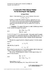
with �t = minf�0;t ; �1;t g and �t = maxf�0;t ; �1;t g. A change of variable as in (3.8), mapping t 2 T to an element t^ 2 S proves that � and � are independent of ht . Finally, changing variables as in (3.9) and using equivalence of norms as in (3.10)-(3.11) yields the result. 2 We now apply Lemmas 2 and 4 to several nite element spaces having hierarchical decompositions. Much of our analysis of these examples comes from the work of Maitre and Musy (1982) [31]. See also Braess (1981) [16]. In these examples, we will compute the constants 1;t , �1;t , and �1;t for the case a = 1, illustrating the e�ect of shape regularity on the estimates. Let t be a triangle with vertices �i, edges �i , and angles �i, 1 � i � 3. �3
�3
t
%
�2
% %t �1
�1
%
t
%e % �3 e t �3
t
et �1 e e �2
% %e
�2
et �2
t
%
%�e3
% e % �1 et% t
�1
�3
e
et �1 %e % �e2
et �2
Fig. 1. Quadratic element (left) and piecewise linear element (right).
In our rst example, we consider the space of continuous piecewise quadratic nite elements, illustrated on the left in Figure 1. Let �i 1 � i � 3 denote the linear basis functions for t. Then Vt = h�i i3i=1 . The space Wt is composed of the quadratic bump functions Wt = h i i3i=1 , where i = 4�j �k , and (i; j; k) is a cyclic permutation of (1; 2; 3). In the second example, we consider the space of continuous piecewise linear polynomials on a re ned mesh, illustrated in Figure 1 on the right. Here Vt contains the linear polynomials on the coarse mesh element t; Vt = h�i i3i=1 , with �i de ned as in the rst example. The space Wt contains the continuous piecewise polynomials on the ne grid that are zero at the vertices of t. Thus Wt = h�^i i3i=1 , where �^i is the standard nodal piecewise linear basis function associated with the midpoint of edge �i of triangle t. By direct computation, we can establish the relation ?jtjr�j � r�k = 21 cot �i = 21 Li:
14
Randolph E. Bank
Let
and
2 L2 + L3 ?L3 ?L2 3 A = 4 ?L3 L3 + L1 ?L1 5 ; ?L2 ?L1 L1 + L2 2L 0 0 3 1 D = 4 0 L2 0 5 :
(3.15)
(3.16) 0 0 L3 Then the element sti�ness matrix for the quadratic hierarchical basis can be shown to be � 2 ?2A=3 � : MQ = ?A= (3.17) 2A=3 4(A + D)=3
We know that
1;t = maxfa(v; w) : jjvjj = jjwjj = 1g = maxf2xt Ay=3 : xt Ax = 2; yt (A + D)y = 3=4g Standard algebraic manipulations yield
12;t = 32 (1 ? �min); where �min is the smallest eigenvalue of the generalized eigenvalue problem Dx = �(A + D)x: (3.18) By direct computation and the use of various trigonometric identities, in particular L1 L2 + L2 L3 + L3 L1 = 1, we can compute detfD ? �(A + D)g = 2(p ? s)�3 + 3(s ? p)�2 ? s� + p = 0; where p = L1 L2 L3 ; s = L 1 + L2 + L 3 : p The corresponding eigenvalues are � = 1 and � = (1 � 4c ? 3)=4, where c = cos2 �1 + cos2 �2 + cos2 �3; and p = 1 ? c: s 3?c Thus
p
(3.19) = 3 + 64c ? 3 : For the second example, the element sti�ness matrix for the piecewise
12;t
Hierarchical Bases and the Finite Element Method
15
linear hierarchical basis is given by
� A=2 ?A � ML = ?A A + D : (3.20) We see that repeating the arguments p for the rst example leads to the same values for 1;t but scaled by 3=2, that is p 3 + 4c ? 3
12;t =
: (3.21) 8 We now turn to the bounds for � and � of Lemma 4. These may be expressed in terms of the largest and smallest eigenvalues in the generalized eigenvalue problem (A + D)x = s�x; (3.22) so that detfA + D ? s�I g = s3 (1 ? �)3 ? s(s2 ? 2)(1 ? �) ? 2p = 0: One can easily write down the analytic solutions of this cubic equation in terms of p and s, but there is no major simpli cation as in the case of 1;t . The bounds for the case of the piecewise linear hierarchical basis are given by �1;t = �min and �1;t = �max. Those for the quadratic case are a simple scaling by 4=3; �1;t = 4�min =3 and �1;t = 4�max =3.
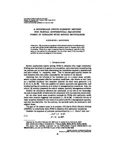
Fig. 2. The contour map for 1 (left) and for �1 =��1 (right). ;t
;t
;t
In Figure 2, we have plotted 1;t and the ratio �?t 1 = �1;t =�1;t as a function of 0 � �1 � � and 0 � �2 � � ? �1 , with �3 = �p? �1 ? �2 . For the case of quadratic elements, the smallest value 1;t = 1= 2 occurs for an equilateral triangle, while the largest value 1;t = 1 occurs for the degenerate cases �i = �j = 0; �k = �. For the case of piecewise linear elements, one should
16
p
Randolph E. Bank
scale all values of 1;t by 3=2; for this case 1;t < 1, even in the degenerate cases. It is the ratio � = �=� that plays a central role in our later analysis. However, we plot the reciprocal to con ne the ratio to the interval [0; 1]. Here the largest value occurs again for the equilateral triangle, where �?t 1 = 1=4, while �t = 0 whenever �i = 0, 1 � i � 3. A special case occurs in the corners of the domain where the function �?t 1 is discontinuous. For example, if one approaches the origin along the edge �1 = 0, then the limiting cubic equation is (1 ? �)3 ? (1 ? �) = 0, with a corresponding �?t 1 = 0. However, if we approach along, say, the line �1 = �2 = �, pthen the limiting cubic is p ? 1 2 (2=3 ? �)(� ? 7�=3 + 4=9) = 0, and �1;t = (7 ? 33)=(7 + 33) > 0.
4. A Posteriori Error Estimates
A posteriori error estimates are now widely used in the solution of partial di�erential equations. A recent survey of the eld is given by Verfurth (1995) [35], which contains a good bibliography on the subject. See also Ainsworth and Oden (1992 and 1993) [1] [2], Babu�ska and Gui (1986) [4], Babu�ska and Rheinboldt (1978a) and (1978b) [6] [7], Bank and Weiser (1985) [14], Weiser (1981) [36], Zienkiewicz et al (1982) [41], and the book edited by Babu�ska et al (1986) [5]. Our discussion here is motivated by Bank and Smith (1993) [13]. A posteriori error estimates provide useful indications of the accuracy of a calculation and also provide the basis of adaptive local mesh re nement or local order re nement schemes. For example, if one has solved a problem for a given p, corresponding to a nite element space M, one can enrich the space to, say, order p + 1 by adding certain hierarchical basis functions to � is the new space, then the set of basis functions already used for M. If M we have the hierarchical decomposition M� = M � W ; where W is the subspace spanned by the additional basis functions. � using the hierarchical basis, If we resolve the problem with the space M one expects intuitively that the component of the new solution lying in M will change very little from the previous calculation. Therefore, the component lying in W should be a good approximation to the error for the solution on the original space M. In fact, for our error estimate, we simply solve an (approximate) problem � to estimate the error. Let u�h 2 M � be the in the space W rather than M nite element solution on the enriched space satisfying a(�uh ; v) = (f; v) (4.1)
Hierarchical Bases and the Finite Element Method
� , and for all v 2 M
jju ? u�hjj = vinf jju ? vjj: 2M�
17
(4.2)
Although we don't explicitly compute u�h , it enters into our theoretical analysis of the a posteriori error estimate for u ? uh . In particular, we assume that the approximate solutions u�h converge to u more rapidly than uh . This is expressed in terms of the saturation assumption jju ? u�hjj � jju ? uhjj; (4.3) � , � 1 is where < 1 independent of h. (We note that since M � M insured by the best approximation property.) In a typical situation, due to � , one can anticipate that the higher degree of approximation for the space M r = O(h ), for some r > 0. In this case, ! 0 as h ! 0, which is stronger than required by our theorems. We seek to approximate the error u ? uh in the space W . Our rst a posteriori error estimator eh 2 W is de ned by a(eh ; v) = (f; v) ? a(uh ; v) (4.4) for all v 2 W . To express this using matrix notation, we consider the linear system of equations corresponding to (4.1), expressed in terms of the hierarchical basis � A A � � U� � � F � 11 12 1 1 (4.5) A21 A22 U�2 = F2 : � expanded The vector (U�1t ; U�2t ) corresponds to the function u�h = v + w 2 M � in terms of the hierarchical basis, with U1 corresponding to v 2 M and U�2 corresponding to w 2 W . In this notation, the linear system solved to compute uh 2 M is given by A11 U1 = F1 . If we combine this with the linear system for eh corresponding to (4.4), we have � A 0 �� U � � F � 11 1 = 1 ; (4.6)
A21 A22
E2
F2
where the vector E2 corresponds to eh 2 W . We begin our analysis by noting the orthogonality relations a(u ? uh; v) = 0 for all v 2 M; (4.7) � a(u ? u�h; v) = 0 for all v 2 M; (4.8) a(�uh ? uh; v) = 0 for all v 2 M; (4.9) a(u ? uh ? eh ; v) = 0 for all v 2 W ; (4.10) a(�uh ? uh ? eh ; v) = 0 for all v 2 W : (4.11) Equations (4.7)-(4.11) are proved using various combinations of (2.4), (2.6), (4.1), and (4.4), restricted to the indicated subspaces. We can use
18
Randolph E. Bank
the orthogonality relationships (4.7)-(4.9) to show jju ? uhjj2 = jju ? u�hjj2 + jju�h ? uhjj2 : (4.12) Using (4.12) in conjunction with the saturation assumption (4.3) shows (1 ? 2 )jju ? uh jj2 � jju�h ? uh jj2 � jju ? uh jj2 ; (4.13) demonstrating u�h ? uh to be a good approximation to the error. However, our goal is to show the easily computed function eh also yields a good approximation of the error. This is shown next. Theorem 1 Let M� = M � W as above and assume (4.3) and Lemma 2 hold. Then (1 ? 2 )(1 ? 2 ) jju ? uh jj2 � jjeh jj2 � jju ? uh jj2 : (4.14) Proof. The right inequality in (4.14) is a simple consequence of (4.10) for the choice v = eh . Now let u�h = u^h + e^h , where u^h 2 M, and e^h 2 W . Then, using (4.9) with v = u^h ? uh and (4.11) with v = e^h , we obtain jju�h ? uhjj2 = a(�uh ? uh; e^h) = a(eh; e^h ): (4.15) Combining this with (4.12), we get jju ? uhjj2 = jju ? u�hjj2 + a(^eh; eh ): (4.16) To complete the proof, we must estimate jje^h jj in terms of jjeh jj. We apply the strengthened Cauchy inequality (3.4) to obtain jju�h ? uhjj2 � jju^h ? uhjj2 + jje^h jj2 ? 2 jju^h ? uhjj jje^h jj � (1 ? 2)jje^h jj2 : (4.17) Combine this with (4.15) to obtain (1 ? 2 )jje^h jj � jjeh jj: (4.18) Using(4.16) and (4.18), we have jju ? uhjj2 � 2 jju ? uhjj2 + 1 ?1 2 jjehjj2 : Rearranging this inequality leads directly to the left-hand inequality in (4.14). 2 We note that computing eh in (4.4) requires the solution of a linear system involving the matrix A22 in (4.6). This is a rather expensive calculation, given that typically the dimension of the space W is much larger than that of M. Therefore it is of great interest to explore ways in which this calculation can be made more e�cient. In situations where Lemma 4 can be applied, one possibility is to replace A22 by its diagonal D22 = diagA22 . In nite element notation, let d(�; �) be the bilinear form corresponding to D22 . If
Hierarchical Bases and the Finite Element Method
19
w = Pj wj �j 2 W , and z = Pj zj �j 2 W , and f�j g are the basis functions
used in Lemma 4, then
d(z; w) =
X j
zj wj a(�j ; �j ):
We compute an approximation e~h 2 W satisfying d(~eh ; v) = (f; v) ? a(uh ; v): (4.19) In our proof of Theorem 1, we replace the orthogonality relations (4.10)(4.11) with a(u ? uh ; v) = d(~eh ; v) for all v 2 W ; (4.20) a(�uh ? uh; v) = d(~eh ; v) for all v 2 W : (4.21) Theorem 2 Let d(�; �) be de ned as above, and assume Theorem 1 and Lemma 4 hold. Then (4.22) �?1 (1 ? 2 )(1 ? 2 ) jju ? uhjj2 � jje~h jj2 � �?1 jju ? uhjj2 : Proof. One can follow the proof of Theorem 1 with small modi cations to show (4.22). However, we will take a more direct approach. From (4.10) and (4.20), we have d(~eh ; v) = a(eh; v) for all v 2 W . Taking v = e~h and v = eh , and applying Lemma 4, we have �jje~h jj2 � jjeh jj2 � �jje~hjj2 : Combining this with Theorem 1 proves (4.22). 2 A second possibility for improving the e�ciency of the computation of the a posteriori error estimate is to use a nonconforming space W� of discontinuous piecewise polynomials to approximate the error. We assume that W � W� , but W� 6� H. The advantage of this approach is that the resulting sti�ness matrix A�22 is block diagonal, with each diagonal block corresponding to a single element. Thus the error can be computed element-by-element by solving a small system for each triangle. To analyze such an error estimator, we need to consider the e�ect of using nonconforming elements. First, we consider the continuous problem. Let E denote the set of interior edges of T . For each edge e 2 E , we denote a xed unit normal ne, chosen arbitrarily from the two possibilities. For w discontinuous along e, let wA and wJ denote the average and jump of w on e, the sign of wJ being chosen consistently with the choice of ne . Let v 2 H[ W� and u be the solution of (2.4). Then a straightforward calculation shows that a(u; v) = (f; v) + g(u; v); (4.23)
20
where
Randolph E. Bank
g(u; v) =
and
XZ e2E e
faru � negAvJ dx;
a(u; v) =
X t2T
(4.24)
a(u; v)t :
The error estimator e�h 2 W� based on this formulation is given by a(�eh ; v) = (f; v) + g(uh ; v) ? a(uh ; v) (4.25) for all v 2 W� . Note that (4.25) consists of a collection of decoupled problems having the appearance of local Neumann problems on each element; since the space W� cannot contain local constants, all problems must be nonsingular and have unique solutions. To analyze this process, we note that the orthogonality conditions (4.10)(4.11) are now replaced by a(u ? uh ? e�h ; v) = g(u ? uh; v) for all v 2 W� ; (4.26) a(�uh ? uh ? e�h ; v) = 0 for all v 2 W : (4.27) � is still the conforming nite element approximation de ned Here u�h 2 M in (4.1). The bilinear form g(�; �) does not appear in (4.27) since vJ = 0 for v 2 W. In examining the proof of Theorem 1, we note that the argument used in proving the left inequality in (4.14) remains unchanged when applied to jje�h jj. The di�culty arises only in the upper bound, where the choice v = e�h in (4.26) leads to jje�h jj2 � jju ? uhjj jje�h jj + jg(u ? uh; e�h)j: Obtaining a bound for the nonconforming term is fairly technical and lengthy, and we will only sketch the arguments here. The interested reader is referred to Bank and Weiser (1985) [14] for a more complete discussion. First note that the presence of the nonconforming term demands more (local) regularity of the solution since line integrals of r(u ? uh) � ne appear. Here we will make the simplifying assumption X 2 2 ht j r (u ? uh )j 2t � �2 jju ? uhjj2 ; (4.28) t2T
which essentially states that a standard a priori estimate for jju ? uh jj is sharp. A more complicated form of the saturation assumption could be used in place of (4.28). Using standard trace inequalities edge-by-edge for e 2 E , we are led to
Hierarchical Bases and the Finite Element Method
the estimate
jg(u ? uh; e�h
)j2
21
! Xp p 2 2 2 2 j ar(u ? uh)j t + ht j ar (u ? uh)j t � C t2T ! X ?2 p 2 p 2 ht j ae�hj t + j are�hj t : t2T
See Brenner and Scott (1994) [20] for a discussion of trace inequalities. Now, using (4.28), and a slight generalization of Lemma 4, � jjwjj2t � h?t 2 j wj 2t � ��jjwjj2t ; for all w 2 Wt , we obtain the bound jg(u ? uh; e�h )j � �jju ? uhjj jje�h jj: Thus we have shown Theorem 3 Let e�h 2 W� satisfy (4.25). Assume (4.3), (4.28), and Lemmas 2 and 4. Then (1 ? 2 )(1 ? 2 ) jju ? uh jj2 � jje�h jj2 � (1 + �)2 jju ? uh jj2 ; (4.29) where and are as in Theorem 1 and � = �(�0 ; 0 ; �0 ; Vr ; Wr ). We remark that one could make the diagonal approximation to the systems of linear equations to be solved in computing e�h . One would then have an estimate modi ed as in Theorem 2. However, there is less advantage to be gained in the current situation because A�22 is already block diagonal with diagonal blocks of small order. Another possibility is to use a di�erent bilinear form b(�; �) in place of a(�; �) on the left-hand side of (4.25). Such a algorithm would calculate e�h 2 W� such that b(�eh ; v) = (f; v) + g(uh ; v) ? a(uh; v): (4.30) One choice suggested by Ainsworth and Oden (1992 and 1993) [1] [2] is to let b(�; �) correspond to the Laplace operator ?�. If there exist nite, positive constants � and � such that �jjwjj2 � b(w; w) � �jjwjj2 in analogy to (3.14), then the analysis of such approximations may be carried out in a fashion similar to Theorem 2. Dur�an and Rodr��guez (1992) [24] and Dur�an, Muschietti and Rodr��guez (1991) [25] analyze the asymptotic exactness of error estimates of the type developed here, a topic we will not consider in detail. We now develop some examples of a posteriori error estimates for the � be the space of space of continuous piecewise linear polynomials. We let M continuous piecewise quadratic polynomials, and W the space of quadratic
22
Randolph E. Bank
bump functions. The basis functions, denoted f i g, will be the standard quadratic nodal basis functions associated with edge midpoints for all edges of the triangulation T . We rst consider the estimate e~h de ned in (4.19). Let X e~h = E~i i: i
Let i be associated with an interior edge e of the triangulation and have support in triangles t1 and t2 , the two triangles sharing edge e. Then + (f; i )t2 ? a(uh ; i )t2 : E~i = (f; i)t1 ? aa((uh;; i ))t1 + i i t1 a( i ; i )t2 Here we see that the calculation of E~i involves only local computations. Standard element-by-element assembly techniques can be used to compute all the relevant quantities. We next consider the computation of e�h in (4.25). Let W� be the space of discontinuous piecewise quadratic bump functions. There are now two basis functions associated with each interior edge, one with support in each element sharing that edge, so the dimension of W� is approximately twice that of W . However, at the level of a single element t, we have Wt = W� t . Let f �i g be the basis for W� . Then the function e�h of (4.25) can be expressed as X e�h = E�i �i: i
Suppose �i , �j , and �k are the three discontinuous quadratic bump functions having support in the element t 2 T . Then we must assemble and solve the 3 � 3 linear system 2 a( � ; � ) a( � ; � ) a( � ; � ) 3 2 E� 3 i it j it i k it 4 a( �i ; �j )t a( �j ; �j )t a( �k ; �j )t 5 4 E�j 5 = E�k a( �i ; �k )t a( �j ; �k )t a( �k ; �k )t
2 (f; � ) ? a(u ; � ) 3 2 g(u ; � ) 3 it h it h it 4 (f; �j )t ? a(uh; �j )t 5 + 4 g(uh ; �j )t 5 : (f; �k )t ? a(uh ; �k )t g(uh ; �k )t
As in the case of e~h , only local computations are involved. All are completely standard except for the evaluation of the nonconforming terms. For example, to evaluate g(uh ; �i )t , we rst note that �i is nonzero on only one edge of t, say edge e. Thus Z g(uh ; �i )t = faruh � ngA �i dx; e
where n is the outward normal for t. To evaluate the average, we must compute aruh for both t and the adjacent triangle sharing edge e.
Hierarchical Bases and the Finite Element Method
23
5. Two-Level Iterative Methods
In this section we analyze several two-level iterations for solving (2.6) (in nite element notation) or, equivalently, (2.7) (in matrix notation). Much of our development is based on Bank and Dupont (1980) [10] and Bank, Dupont, and Yserentant (1988) [11]. See also the books of Hackbusch (1985) [30] and Bramble (1993) [17]. Let M = V � W , let A be the sti�ness matrix computed using the hierarchical basis, and partitioned according to (2.8), and let A = L + D + Lt ; (5.1) where � � � � D = A011 A0 and L = A0 00 : 22
21
We consider the following iteration for solving (2.6). Let u0 2 M be given. We de ne the sequence uk = vk + wk , with vk 2 V and wk 2 W by a(vk+1 ? vk ; �) = !f(f; �) ? a(uk ; �)g (5.2) for � 2 V , and a(wk+1 ? wk ; �) = !f(f; �) ? a(uk ; �)g (5.3) for � 2 W . The iteration (5.2)-(5.3) can be written in matrix notation as D(xk+1 ? xk ) = !fF ? Axk g; (5.4) where the vector xk 2 IRN corresponds to the nite element function uk 2 M. Equations (5.2)-(5.4) represent a standard block Jacobi iteration for solving (2.6)-(2.7) Although we have written (5.4) as a stationary iteration, practically we expect to use D as a preconditioner in the conjugate gradient procedure. We refer the interested reader to Golub and Van Loan (1983) [27] or Golub and O'Leary (1989) [28] for a complete discussion of the preconditioned conjugate gradient algorithm. Here we analyze the generalized condition number of the preconditioned system. Theorem 4 Let A = L + D + Lt as de ned above. Then for all x 6= 0, 1 � xt Dx � 1 ; (5.5) 1 + xt Ax 1 ? where 0 � < 1 is given in Lemma 2. Proof. It is easiest to analyze (5.5) using nite element notation. Let u = v + w, with v 2 V and w 2 W , correspond to x 2 IRN . Then xt Ax = jjujj2 and xt Dx = jjvjj2 + jjwjj2 : Now jjujj2 = jjvjj2 + jjwjj2 + 2a(v; w):
24
Randolph E. Bank
Applying Lemma 2, we have (1 ? )(jjvjj2 + jjwjj2 ) � jjujj2 � (1 + )(jjvjj2 + jjwjj2 ); proving (5.5). 2 The generalized condition number K is given by K = 11 ?+
: The optimum value for ! for the stationary iteration (5.4) is ! = 1, and the rate of convergence is given by K ? 1 = : K+1 See Dupont, Kendall and Rachford (1968) [23] for an analysis of the stationary method. If conjugate gradient acceleration is used, the estimate for the rate of convergence is bounded by p pK ? 1 = p 2 : K+1 1+ 1? We note that (5.4) requires the solution of linear systems involving the diagonal blocks A11 and A22 in each iteration. We next show that the systems involving A22 can be e�ectively solved using an inner iteration. Those involving A11 should either be solved directly, or solved recursively, using a multilevel iteration. Let A^22 be a symmetric, positive de nite preconditioner for A22 , and suppose we approximately solve the linear system A22 x = b, using m � 1 steps of the iterative process A^22 (xk+1 ? xk ) = b ? A22 xk : (5.6) The iteration (5.6) should not be accelerated, but should be implemented as a stationary iteration to allow the use of conjugate gradient acceleration for the overall (outer) iteration. We assume that any xed parameters for (5.6) have been already incorporated in the de nition of A^22 . Let G = I ? A122=2 A^?221 A122=2 : We assume G is symmetric with
Let
j Gj `2 = � < 1:
(5.7)
Rm = Gm(I ? Gm)?1 :
(5.8)
Hierarchical Bases and the Finite Element Method
The eigenvalues of Rm lie on the interval
m
0 � � � 1 ?� �m
25
(5.9)
when m is even or if all eigenvalues of G are nonnegative. In the latter case, G is sometimes called a smoother. If G is not a smoother and m is odd, we must use the weaker bound m m (5.10) ? 1 +� �m � � � 1 ?� �m :
A induction argument shows the m-step process in (5.6) is mathematically equivalent to the solution of A122=2 (I + Rm )A122=2 xm = b + A122=2 Rm A122=2 x0 : (5.11) In our current situation, the initial guess x0 = 0, simplifying the right hand side of (5.11). Our overall preconditioner, using m inner iterations, is thus " # 0 0 ^ D = D + 0 A1=2 R A1=2 : (5.12) 22 m 22 Theorem 5 Let A = L + D + Lt and D^ be de ned as above. Then for all x 6= 0, ^ 1 xt Dx 1 � � (5.13) m t (1 + )(1 + � ) x Ax (1 ? )(1 ? �m ) : Proof. As in the proof of Theorem 4, we let u = v + w 2 M correspond to x 2 IRN . Then ^ � jjvjj2 + (1 ? �m )?1 jjwjj2 : jjvjj2 + (1 + �m )?1jjwjj2 � xt Dx Thus ^ 1 ; 1 � xt Dx � m t 1+� x Dx 1 ? �m and the theorem follows from Theorem 4 and t Dx ^ ^ ! xt Dx ! xt Dx x xt Ax = xt Dx xt Ax :
2
The generalized condition number K is bounded by � 1 + � � 1 + �m � K � 1 ? 1 ? �m : Here we see that the use of inner iterations has only a modest e�ect on the generalized condition number, provided that � is small or m is large.
26
Randolph E. Bank
^ t Ax directly, instead of bounding We remark that by bounding xt Dx=x ^ t Dx and xt Dx=xt Ax separately, one can achieve a somewhat smaller xt Dx=x but more complicated bound for K. If G is a smoother, then the bound on K can be improved to � � �� K � 11 +?
1 ?1�m : We now consider the symmetric block Gauss-Seidel iteration (D + L)(xk+1=2 ? xk ) = F ? Axk (5.14) t (D + L )(xk+1 ? xk+1=2 ) = F ? Axk+1=2 : In nite element notation, we may write (5.14) as a(vk+1=2 + wk ; �) = (f; �) (5.15) for � 2 V , a(vk+1=2 + wk+1 ; �) = (f; �) (5.16) for � 2 W , and a(vk+1 + wk+1 ; �) = (f; �) (5.17) for � 2 V . A careful analysis of (5.15)-(5.17) will show that block GaussSeidel and block symmetric Gauss-Seidel are equivalent as stationary iterative methods (i.e. vk+1=2 = vk ), but this is no longer true when symmetric Gauss-Seidel is used as a preconditioner for the conjugate gradient algorithm. Let ek = x ? xk . Then from (5.14), ek+1=2 = fI ? (D + L)?1 Agek ; ek+1 = fI ? (D + L)?t Agek+1=2 ; from which it follows that ek+1 = fI ? (D + L)?t AgfI ? (D + L)?1 Agek = fI ? [(D + L)?t + (D + L)?1 ]A + (D + L)?t A(D + L)?1 Agek = fI ? (D + L)?t (L + 2D + Lt ? A)(D + L)?1 Agek (5.18) ? t ? 1 = fI ? (D + L) D(D + L) Agek = fI ? B ?1 Agek ; where B = (D + L)D?1 (D + Lt ) = A + LD?1 Lt : (5.19) Once again, our task is to determine the generalized condition number by estimating the Rayleigh quotient.
Hierarchical Bases and the Finite Element Method
27
Theorem 6 Let A = L + D + Lt as de ned above, and let B be given by (5.19). Then
t 1 ; 1 � xxtBx � Ax 1 ? 2
(5.20)
xt LD?1 Lt x : � = max x6=0 xt Ax
(5.21)
where 0 � < 1 is given in Lemma 2. Proof. Since LD?1 Lt is symmetric, positive semide nite, it is clear from (5.19) that the lower bound is one. The upper bound is given by 1+ � where This can be written as where
yt Dy ; � = max x6=0 xt Ax Dy = Lt x:
In nite element notation, this becomes
jjv^jj2 ; � = max u6=0 jjujj2
(5.22)
where u = v + w, v 2 V , w 2 W and v^ 2 V satis es a(^v; �) = a(w; �) (5.23) for all � 2 V . Written in nite element language, (5.22)-(5.23) is easy to analyze in terms of the strengthened Cauchy inequality. We take � = v^ in (5.23) to see jjv^jj � jjwjj: On the other hand jjujj2 = jjvjj2 + jjwjj2 + 2a(v; w) � jjvjj2 + jjwjj2 ? 2 jjvjj jjwjj � (1 ? 2 )jjwjj2 � (1 ? 2 ) ?2jjv^jj2 : The theorem now follows from combining this estimate and (5.22). 2 The analysis of the block symmetric Gauss-Seidel scheme with inner iterations is a little more complicated. We formally consider the iteration (D^ + L)(xk+1=2 ? xk ) = F ? Axk ; (5.24) (D^ + Lt )(xk+1 ? xk+1=2 ) = F ? Axk+1=2 ;
28
Randolph E. Bank
where D^ is given in (5.12). A calculation similar to (5.18) shows that ek+1 = fI ? (D^ + L)?t AgfI ? (D^ + L)?1 Agek = fI ? [(D^ + L)?t + (D^ + L)?1 ]A + (D^ + L)?t A(D^ + L)?1 Agek = fI ? (D^ + L)?t (L + 2D^ + Lt ? A)(D^ + L)?1 Agek (5.25) ? t ? 1 ^ ^ ^ = fI ? (D + L) (2D ? D)(D + L) Agek = fI ? B^ ?1 Agek ; where B^ = (D^ + L)(2D^ ? D)?1 (D^ + L)t = A + (D ? D^ + L)(2D^ ? D)?1 (D ? D^ + L)t (5.26) ? 1 t = A + LD L + �: Here # # " " 0 0 0 0 ; = �= 0 A122=2 R2m A122=2 0 A122=2 Rm2 (I + 2Rm )?1 A122=2 and Rm is de ned in (5.8). Theorem 7 Let A = L + D + Lt as de ned above, and let B^ be given by (5.26). Then t^ 1 1 � xxtBx � (5.27) 2 Ax (1 ? )(1 ? �2m ) ; where 0 � < 1 is given in Lemma 2, and � is given in (5.7). Proof. Since LD?1 Lt + � is symmetric, positive semide nite, the lower bound is one. For the upper bound, xt LD?1 Lt x=xt Ax was estimated in the proof of Theorem 6. Let u = v + w 2 M correspond to x 2 IRN . Then, using (5.7)-(5.8) and Lemma 2, we have ! ! xt �x � �2m jjwjj2 � �2m � 1 � : xt Ax 1 ? �2m jjujj2 1 ? �2m 1 ? 2 Combining these estimates, we have 2 ! 2m ! � 1 � ^
� 1 xt Bx � 1 + + = t 2 2 m 2 2 x Ax 1? 1?� 1? (1 ? )(1 ? �2m ) :
2
We now consider some possibilities for the inner iterations. One obvious choice is a Jacobi method based on the diagonal matrix D22 = diagA22 with A^22 = D22 =!. Using Lemma 4, for the choice ! = 2=(� + �), we have 1; � � �� ? +1
Hierarchical Bases and the Finite Element Method
29
where � = �=�. A second possibility is to use a symmetric Gauss-Seidel iteration. Let A22 = L22 + D22 + Lt22 , where L22 is lower triangular. We then take ?1 (D22 + L22 )t : A^22 = (D22 + L22 )D22 (5.28) Lemma 5 Suppose the hypotheses of Lemma 4 hold, and let A^22 be given by (5.28). Then there exists a nite positive constant � depending only on �0 , 0 , and �0, such that t A^22 x (5.29) 1 � xxt A x � 1 + �: 22
?1 Lt , Proof. As usual, the lower bound is one, since A^22 = A22 + L22 D22 22 ? 1 t and L22 D22 L22 is symmetric and positive semide nite. Now
yt D22 y ; � = max x xt A x 22
where
D22 y = Lt22 x:
In nite element notation, this is
P w^2 jj� jj2 j j j ; � = max w jjwjj2 where w^ 2 W corresponds to y, w 2 W corresponds to x, and f�j g are the basis functions for W . Since the basis functions for W are developed from
a xed set of functions de ned on the reference element, the support of a given basis function can intersect that of only a small number of other basis functions (there are at most a xed number of nonzeros in any row of Lt22 , independent of the number of elements in the mesh). Therefore we must have X 2 2 X 2 2 w^j jj�j jj � C wj jj�j jj ; j
j
where C = C (�0 ). The result now follows directly from Lemma 4. 2 Using Lemma 5, we can estimate � = j I ? A122=2 A^?221 A122=2 j `2 � 1 +� � :
Thus we see that although these inner iterations perturb the rate of convergence, they do not a�ect the essential feature that the rate depends only on local properties of the nite element spaces, and is independent of such things as the dimension of the space, uniformity or nonuniformity of the mesh, and regularity of the solution.
30
Randolph E. Bank
6. Multilevel Cauchy Inequalities
In this section we will develop several strengthened Cauchy inequalities of use in analyzing hierarchical basis iterations with more than two levels. These estimates are developed for the special case of continuous piecewise linear nite elements; they can be combined with the two-level analysis of Section 5 to develop multilevel algorithms for higher degree polynomial spaces. We will return to this point in Section 7. Much of the material here is based on Bank and Dupont (1979) [9], Yserentant (1986) [39], and Bank, Dupont and Yserentant (1988) [11]. See also the books of Hackbusch (1985) [30], Bramble (1993) [17], and Oswald (1994) [33]. Let T1 be a coarse, shape regular triangulation of . We will inductively construct a sequence of uniformly re ned triangulations Tj , 2 � j � k, as follows. For each triangle t 2 Tj ?1, we will construct 4 triangles in Tj by pairwise connecting the midpoints of t. All triangulations will be shape regular, as every triangle t 2 Tj will be geometrically similar to the triangle in T0 which contains it. We could also allow nonuniform re nements that control shape regularity, for example those of the type used in the adaptive nite element program PLTMG (Bank (1994) [8]). See also Rude (1993) [34] and Deu hard, Leinen and Yserentant (1989) [22]. With this de nition, it is easy to introduce the notion of the level of a given vertex in the triangulation Tj . All vertices in the original triangulation T1 are called level-1 vertices. The new vertices created in forming Tj from Tj?1 are called level-j vertices. Notice that all vertices in Tj have a level less than or equal to j . Also note that each vertex has a unique level, and this unique level is the same in all triangulations that contain it. Let Mj be the space of continuous piecewise linear polynomials associated with Tj . Functions in Mj will be represented using the hierarchical basis, which is easily constructed in an inductive fashion. Let f�i gNi=11 denote the usual nodal basis functions for the space M1 ; this is also the hierarchical basis for M1 . To construct the hierarchical basis for Mj , j > 1, we take the union of the hierarchical basis for Mj ?1 , f�i giN=1j?1 , with the nodal basis functions associated with the newly introduced level j vertices, f�i gNi=jNj?1 +1 . Let Vj be the subspace spanned by the basis functions associated with the level-j vertices, f�i gNi=jNj?1 +1 , where N0 = 0. Note that V1 = M1 . Then we can write for j > 1,
Mj = Mj?1 � Vj = V1 � V2 � : : : � Vj : Let Nj , 1 � j � k ? 1 be de ned by
Nj = Vj+1 � Vj+2 � : : : � Vk
Hierarchical Bases and the Finite Element Method
31
with Nk = ;. Then we have the decompositions Mk = Mj � Nj for 1 � j � k. Before proceeding to the Cauchy inequalities, we need a preliminary technical result. Lemma 6 Let t 2 S , where S is de ned as in Section 2. Let T 0 be a shape regular triangulation of t, whose elements have a minimum diameter of h. Let M0 be the space of continuous piecewise linear polynomials associated with T 0 . Then there exists a constant c = c(�0 ), independent of h, such that, for all v 2 M0 , j vj 1;t � cj log hj1=2 j vj 1;t : (6.1) Proof. Here we will only sketch a proof, following ideas in Bank and Scott (1989) [12], but see Yserentant [39] (1986) for a more detailed, but also more elementary proof. We remark that estimate (6.1) is restricted to two space dimensions. Our proof is based on an inverse inequality, and the Sobolev inequality; see Brenner and Scott (1994) [20] or Ciarlet (1980) [21] for a general discussion of these topics. Let t0 be a shape regular triangle of size ht0 , and let v be a linear polynomial. The inverse inequality we require states
j vj L1 (t0 ) � C0h?t0 2=p j vj Lp(t0 )
for 1 � p � 1. Let D be a closed bounded region with a piecewise smooth boundary; then the Sobolev inequality we need states
j vj Lp (D) � C1 ppj vj H1 (D) for all v 2 H1 (D) and all p < 1. Now let t 2 S and v 2 M0 ; then j vj L1(t) = tmax 0 2T 0 j v j L1 (t0 ) � C0h?2=p tmax 0 2T 0 j v j Lp (t0 ) � C0h?2=pj vj Lp (t) � C0C1h?2=p ppj vj H1 (t) The proof is now completed by taking p � ?4 log h. 2 Lemma 7 Let Mk = Mj � Nj as above. Then there exist positive constants j , 1 � j � k ? 1 such that (6.2)
j � 1 ? k ?c j ;
32
Randolph E. Bank
and the strengthened Cauchy inequality ja(v; w)j � j jjvjj jjwjj (6.3) holds for v 2 Mj and w 2 Nj . The positive constant c in (6.2) is independent of j and k. Proof. Our proof is based on that of Bank and Dupont (1979) [9]. Following the pattern used in proving Lemma 2, we rst reduce the estimate (6.3) to an elementwise estimate for t 2 Tj . If we show ja(v; w)t j � j;tjjvjjt jjwjjt ; (6.4) then
j = max
: t2T j;t j
Let t 2 Tj , and let xi , 1 � i � 3 denote the three vertices of t. We map t to a triangle t^ 2 S using the change of variable
x^ = x ?h x1 : t
As in the proof of Lemma 2, this veri es that j;t is independent of ht . Notice that Mj;t , the restriction of Mj to t, is just the space of linear polynomials on t and has dimension three. In the case of uniform re nement, the space Nj;t is the space of piecewise linear polynomials on a uniform grid of 4k?j congruent triangles, which are zero at the three vertices of t. The (local) constant function is thus contained in Mj;t , and Mj;t �Nj;t is just the space of continuous piecewise linear polynomials on t. Let v 2 Mj;t and w 2 Nj;t. Then
j;t = jjvjj max a(v; w)t =jjwjj =1 t
t
t
t
jjv ? wjjt = jjvjj max 1 ? 2 t =jjw jjt =1 � jjvjj max 1 ? cj v ? wj 21;t ; =jjwjj =1 2
where c = c(�0 ; 0 ). We now apply Lemma 6, noting that h � 2k?j for the triangulation of t^.
C j v ? wj 21;t
j;t � jjvjj max 1 ? log 2k?j ; t =jjw jjt =1 where C = C (�0 ; 0 ; �0 ). Next we note that, since v is just a linear polynomial on t with jjvjjt = 1, and w(xi ) = 0, 1 � i � 3, we have a xed constant c0 > 0, independent of j
Hierarchical Bases and the Finite Element Method
33
and k, such that c0 < max xi jv(xi )j = max xi jv(xi ) ? w(xi )j � j v ? wj 1;t : Thus it follows that
0
j;t � 1 ? logCc2k?j ;
and the lemma follows. 2 We next describe the result of Lemma 7 in terms of interpolation operators. Lemma 8 Let u = vj + wj 2 Mk , vj 2 Mj and wj 2 Nj . De ne the interpolation operator Ij , mapping Mk to Mj , by Ij (u) = vj . Then p (6.5) jjIj (u)jj � C k ? j jjujj: The positive constant C is independent of j and k. Proof. Apply Lemmas 3 and 7. See also Yserentant (1986) [39], and Bank, Dupont and Yserentant (1988) [11]. 2 We nish this section with Lemma 9 Let Vi and Vj for 1 � i; j � k be de ned as above. Then there exist positive constants ?i;j satisfying ?i;j � c2?ji?j j=2 ; (6.6) such that ja(v; w)j � ?i;j jjvjj jjwjj (6.7) for all v 2 Vi and w 2 Vj . The constant c in (6.6) is independent of i and j . Proof. Our proof is similar to that given by Yserentant (1986) [39]. Without loss of generality, suppose i < j . We need to consider no triangulation ner than Tj , since subsequent re nements do not a�ect either v or w. As in the other Cauchy inequalities, one rst reduces the estimate to a single element t 2 Ti , that is ja(v; w)t j � ?i;j;tjjvjjt jjwjjt : (6.8) We then consider the gradient terms and the lower order terms separately as in (3.6)-(3.7). For the highest order term, we must again consider the special importance of the (local) constant function, which in this case belongs to Vi;t. Following the pattern in the proof of Lemma 2, we next map t 2 Ti to an element t^ 2 S by scaling and translation, showing that the estimate must be independent of ht . Also note that under this mapping, triangles in Tj become triangles with size h^ � 2i?j .
34
Randolph E. Bank
The central estimate is to show that ja(^v; w^)1;t^j � ?i;j;1;tjjv^jj1;t^jjw^jj1;t^; where Z a(^v; w^)1;t^ = ^ a^rv^ � rw^ d^x t jjv^jj21;t^ = a(^v; v^)1;t^: We will also use the norms Z Z 2 2 2 j v^j t^ = ^ v^ d^x and j v^j @t^ = ^ v^2 d^x: t
(6.9)
@t
The function v^ is just a linear polynomial on t^, while w^ is a piecewise linear polynomial vanishing at all the vertices with level smaller than j . Such a function is necessarily very oscillatory, and for such a function the di�erential operator behaves very much like h^ ?1 times the identity operator. In particular, we have the estimates j w^j t^ � C ^hjjw^jj1;t^ � C^ 2i?j jjw^jj1;t^ (6.10) and j w^j @t^ � C ^h1=2 jjw^jj1;t^ � C^ 2(i?j)=2 jjw^jj1;t^; (6.11) where C^ = C^ (�0 ; �0 ). Now, using integration by parts, the fact that �v = 0 in t^, and (6.10)(6.11) we have
Z ?r a ^ � r v ^ w ^ d^ x + a^rv^ � nw^ d^s t^ @ t^ � C fjjrv^j t^j wj t^ + j rv^j @t^j w^j @t^g � C 02(i?j)=2 jjv^jj1;t^jjw^jj1;t^:
a(^v; w^)1;t^ =
Z
The lower order term is easy to treat in this case because of (6.10). 2
7. Multilevel Iterative Methods
In this section, we will analyze block Jacobi and block symmetric GaussSeidel iterations using the hierarchical decomposition Mk = V 1 � V 2 � : : : � V k de ned in Section 6. Much of this material comes from Bank, Dupont and Yserentant (1988) [11], but see also Bramble (1993) [17], Bramble, Pasciak, and Xu (1990) [19], Bramble, Pasciak, Wang, and Xu (1991) [18], Griebel (1994) [29], Hackbusch (1985) [30], Ong (1989) [32], Xu (1989) and (1992) [37] [38], and Yserentant (1986) and (1992) [39] [40].
Hierarchical Bases and the Finite Element Method
35
As before, we let f�i gNi=jNj?1 +1 denote piecewise linear nodal basis functions for the level-j vertices in Tk . Then the sti�ness matrix A can be expressed as the symmetric, positive de nite block k � k matrix
2 A11 A12 � � � A1k 3 6A A A 7 (7.1) A = 664 ..21 22 . . ..2k 775 ; . . . Ak1 Ak2 � � � Akk where Ajj is the (Nj ? Nj ?1 ) � (Nj ? Nj ?1 ) matrix of energy inner products
involving just the level-j basis functions. In similar fashion to the analysis in Section 5, we set A = L + D + Lt ; (7.2) where 3 2 0 3 2 A11 77 66 A21 0 77 6 A22 and L = D = 664 6 7 . . . . 75 : ... 4 .. 5 Ak1 Ak2 � � � 0 Akk We rst consider the block Jacobi iteration. Let u0 2 Mk be given. We de ne the sequence ui = v1;i + v2;i + : : : + vk;i ; where vj;i 2 Vj , 1 � j � k. In nite element notation, the block Jacobi iteration is written a(vj;i+1 ? vj;i ; �) = !f(f; �) ? a(ui ; �)g (7.3) for � 2 Vj , 1 � j � k. The iteration (7.3) can be written in matrix notation as D(xi+1 ? xi) = !fF ? Axi g; (7.4) where the vector xi 2 IRNk corresponds to the nite element function ui 2 Mk . To estimate the rate of convergence, we must bound the Rayleigh quotient t
� 0 < � � xxtDx Ax � �
(7.5)
for x 6= 0. In nite element notation, this is written
Pk jjv jj2 i � 0 < � � i=1 jjvjj2 � �; P 6 0. where vi 2 Vi and v = ki=1 vi =
(7.6)
36
Randolph E. Bank
For any v = v1 + v2 + : : : + vk , we de ne zj = v1 + v2 + : : : + vj ; (7.7) for 1 � j � k, with z0 = 0, wj = vj+1 + vj+2 + : : : + vk ; (7.8) for 0 � j � k ? 1, with wk = 0. Thus we have v = zj + wj , 0 � j � k. Note zj 2 Mj , while wj 2 Nj . We begin our analysis with an upper bound for (7.6). First note that the angle between the spaces V1 � V2 � : : : � Vj ?1 = Mj ?1 and Vj is just the angle between the spaces V and W of Lemma 2. Therefore the constant in the strengthened Cauchy inequality for these spaces, which we will denote by ~ , does not depend on j . Now jjzj jj2 = jjzj?1 + vj jj2 = jjzj ?1 jj2 + jjvj jj2 + 2a(zj ?1 ; vj ) � jjzj?1 jj2 + jjvj jj2 ? 2~ jjzj?1 jj jjvj jj � (1 ? ~2 )jjvj jj2 : We now use Lemma 7 to deduce jjvjj2 = jjzj + wj jj2 = jjzj jj2 + jjwj jj2 + 2a(zj ; wj ) � jjzj jj2 + jjwj jj2 ? 2 j jjzj jj jjwj jj � (1 ? j2)jjzj jj2 � (1 ? j2)(1 ? ~2)jjvj jj2 : Thus we have k k 2 X X jjvijj2 � 1jj?vjj ~2 1 ?1 2 � Ck2jjvjj2 : i i=1 i=1 To nd a lower bound, we note that
jj
k X i=1
vi jj2
=
k X k X
i=1 j =1
a(vi ; vj ) �
k X k X
i=1 j =1
?i;j jjvi jj jjvj jj = E t ?E;
where Ei = jjvi jj, and ? is the k � k matrix introduced in Lemma 9. One can easily see that j ?j `2 < C , so that
jjvjj2 = jj Thus we have proved
k X i=1
vijj2 � C
k X i=1
jjvi jj2 :
Hierarchical Bases and the Finite Element Method
Theorem 8 Let A = L + D + Lt as de ned above. Then t 2 C1 � xxtDx Ax � C2 k ;
37
(7.9)
where Ci = Ci (�0 ; 0 ; �0 ), i = 1; 2. Note that the generalized condition number K � ck2 now depends on the number of levels. For the case of uniform re nement, k = O(log Nk ), so this p introduces a logarithmic-like term into the convergence rate. Note that K � c~k, so that conjugate gradient acceleration can be expected to have a more signi cant impact on the k-level iteration than on the two-level method. As in the case of the two-level iteration, we may solve linear systems of the form Aii x = b by an inner iteration for all i > 1. Following the development given in Section 5, let A^ii be the preconditioner for Aii and let Gi = I ? A1ii=2 A^?ii 1 A1ii=2 . Suppose max j G j = � < 1; i>1 i `2 and assume for simplicity that m � 1 inner iterations are used for all i > 1. Let Ri;m = Gmi (I ? Gmi )?1 . Then, using reasoning similar to that of (5.12), we replace (7.4) with D^ (xi+1 ? xi ) = !fF ? Axig (7.10) where 3 20 77 1=2 6 R2;m D^ = D + D1=2 664 75 D = D + Z: ...
Rk;m
Theorem 9 Let A = L + D + Lt and D^ be de ned as above. Then ^ C2k2 ; C1 � xt Dx � (7.11) 1 + �m xt Ax 1 ? �m
where Ci , i = 1; 2 are given in Theorem 8. Proof. Following the proof of Theorem 5, we see for all x 6= 0 , ^ 1 1 � xt Dx m t 1+� x Dx � 1 ? �m : The theorem then follows easily from this estimate and Theorem 8. 2 We next consider the symmetric block Gauss-Seidel iteration. In nite element notation, we may write this as a(vj;i+1=2 ? vj;i; �) = (f; �) ? a(zj?1;i+1=2 + wj?1;i ; �) (7.12)
38
Randolph E. Bank
for � 2 Vj , j = 1; 2; : : : ; k, and a(vj;i+1 ? vj;i+1=2 ; �) = (f; �) ? a(zj;i+1=2 + wj;i+1 ; �) (7.13) for � 2 Vj , j = k; k ? 1; : : : ; 1. Here zj;i and wj;i are de ned analogously to vj and wj in (7.7)-(7.8). In matrix notation the iteration is written (D + L)(xi+1=2 ? xi ) = F ? Axi ; (7.14) t (D + L )(xi+1 ? xi+1=2 ) = F ? Axi+1=2 : As in the two-level scheme, the preconditioner B is given by B = (D + L)D?1 (D + Lt ) = A + LD?1 Lt : (7.15) Theorem 10 Let A = L + D + Lt and B be de ned as above. Then t
where
1 � xxtBx Ax � 1 + �;
(7.16)
� � C3 k 2 ;
(7.17)
and C3 = C3 (�0 ; 0 ; �0 ). Proof. The lower bound is clear since LD?1 Lt is symmetric and positive semide nite. For the upper bound, we estimate where
yt Dy � = max x6=0 xt Ax
Dy = Lt x: Let v = v1 + v2 + : : : + vk = zj + wj , with vi 2 Vi and zj 2 Mj and
wj 2 Nj as in (7.7)-(7.8). Then in nite element notation, we have Pk?1 jjv~ jj2 i=1 i ; � = max (7.18) v6=0 jjvjj2 where
a(~vi ; �) = a(wi; �)
for all � 2 Vi . Taking � = v~i in (7.19) and applying Lemma 7, we have jjv~i jj � i jjwijj; and jjvjj2 = jjzi + wijj2 = jjzi jj2 + jjwi jj2 + 2a(zi ; wi )
(7.19)
Hierarchical Bases and the Finite Element Method
39
� jjzi jj2 + jjwijj2 ? 2 i jjzi jj jjwi jj � (1 ? i2)jjwi jj2 � (1 ? i2) i?2 jjv~i jj2 :
Thus we have
��
2
kX ?1
i2 < C k2 : 3 2 i=1 1 ? i
We next analyze the e�ect of inner iterations on the symmetric block Gauss-Seidel iteration. Thus we replace D with D^ in (7.14) and obtain the iteration (D^ + L)(xi+1=2 ? xi ) = F ? Axi (7.20) t (D^ + L )(xi+1 ? xi+1=2 ) = F ? Axi+1=2 Following arguments similar to (5.26), we have B^ = (D^ + L)(2D^ ? D)?1 (D^ + Lt ) = A + (D ? D^ + L)(2D^ ? D)?1 (D ? D^ + Lt ) (7.21) ? 1 t = A + (L ? Z )(D + 2Z ) (L ? Z ): ^ t Ax. Since As usual, we need to estimate the Rayleigh quotient xt Bx=x (L ? Z )(D + 2Z )?1 (Lt ? Z ) is symmetric, positive semide nite, the lower bound is just 1. To obtain an upper bound, the essential estimate we must make is t ?1 t �^ = max x (L ? Z )(D + 2Z ) (L ? Z )x
xt Ax = j (D + 2Z )?1=2 (Lt ? Z )A?1=2 j 2`2 � � j (D + 2Z )?1=2 D1=2j `2 j D?1=2 LtA?1=2 j `2 �2 +j (D + 2Z )?1=2 ZD?1=2 j `2 j D1=2 A?1=2 j `2 : x6=0
Now and
m
j (D + 2Z )?1=2 D1=2j `2 � 11 ?+ ��m 2m
j (D + 2Z )?1=2 ZD?1=2j `2 � 1 ?� �2m :
The norms j D?1=2 Lt A?1=2 j `2 and j D1=2 A?1=2 j `2 are estimated using Theorems 10 and 8, respectively. Combining these estimates, we have
40
Randolph E. Bank
Theorem 11 Let A = L + D + Lt and B^ be de ned as above. Then t^ 1 � xxtBx (7.22) Ax � 1 + �^;
where
0s s 2m 12 m 1 + � �^ � @ 1 ? �m C3 + 1 ?� �2m C2A k2 � C4 k2 ;
(7.23)
and C2 and C3 are given in Theorems 8 and 10, respectively. If G is a smoother, then using (5.9) we have j (D + 2Z )?1=2 D1=2 j `2 � 1, and the improved estimate
0 s 2m 12 p �^ � @ C3 + 1 ?� �2m C2A k2 � C4 k2 :
We conclude with several remarks about the two-level and k-level methods. Although the k-level method was developed for only the case of continuous piecewise linear polynomials, this is su�cient to construct e�cient methods for higher-degree spaces. For example, we consider the case of continuous piecewise quadratic polynomials on a sequence of meshes Tj , 1 � j � k. At rst glance, one might be tempted to try to develop a method in which one used piecewise quadratic spaces on all levels. Further re ection would lead one to the conclusion that such a method could potentially be very complicated, as it is not clear that there is a simple way to develop a hierarchical basis. It is also not clear that the analysis of such a method could be based on the results in this work. On the other hand, we could begin by making the usual two-level decomposition M = V � W , where V is the space of piecewise linear polynomials on Tk and W is the space of piecewise quadratic bump functions that are zero at the vertices of Tk . The dimension of W is then approximately 3N=4 where N is the dimension of M. For the space V , which is just the space of piecewise linear polynomials on Tk , we can make the hierarchical decomposition V = V 1 � V2 � : : : � V k as described here. Overall, we have the hierarchical decomposition M = V 1 � V2 � : : : � V k � W : Based on this decomposition, there is an obvious multilevel hierarchical basis iteration that can be developed. This iteration could be viewed as a two-level iteration, with an elaborate k-level inner iteration used to solve the linear systems associated with the space V . Alternatively, this iteration could be viewed as a k + 1 level iteration, in which the the rst k levels are the
Hierarchical Bases and the Finite Element Method
41
standard ones, but level k +1 is special, in that the degree of approximation is increased instead of the mesh being re ned. For either viewpoint, the algorithm is the same, and its analysis is straightforward using the results in Sections 3-7. Another possibility along these lines is to make some further hierarchical decomposition of the space W . For example, suppose now that M is the space of continuous piecewise quartic polynomials on Tk . We can begin by making a decomposition M = V � W , where V is the space of continuous piecewise linear polynomials and W is the space of quartic polynomials that are zero at the vertices of Tk . We make a further decomposition of V as in the previous example. We can also conveniently make the further decomposition W = W2 �W4 , where W2 is the space of continuous piecewise quadratic polynomials that are zero at the vertices of Tk . This is the same as the space W in our last example. The space W4 is now the space of continuous piecewise quartic polynomials that are zero at the vertices and edge midpoints of Tk (i.e. all the nodes associated with the piecewise linear and piecewise quadratic spaces). This space can be characterized in terms of a subset of the standard nodal basis functions for the piecewise quartic space, the bump functions associated with the 1=4 and 3=4 points on each edge, and the bubble functions associated with the barycentric coordinates (1=4; 1=4; 1=2), (1=4; 1=2; 1=4), and (1=2; 1=4; 1=4) in each element. This leads to an overall decomposition M = V 1 � V2 � : : : � V k � W 2 � W 4 : The resulting hierarchical basis iteration could then be viewed as a basic two-level iteration in which elaborate inner iterations are used for solving linear systems associated with both the V and W spaces, or as a k + 2 level scheme in which the last two levels involve an increase in degree of approximation rather than a re nement of the mesh.
REFERENCES
Mark Ainsworth and J. Tinsley Oden. A procedure for a posteriori error estimation for h-p nite element methods. Comp. Meth. Appl. Mech. Engrg., 101:73{96, 1992. Mark Ainsworth and J. Tinsley Oden. A uni ed approach to a posteriori error estimation using element residual methods. Numerische Mathematik, 65:23{ 50, 1993. A. K. Aziz and I. Babu�ska. Part I, survey lectures on the mathematical foundations of the nite element method. In The Mathematical Foundations of the Finite Element Method with Applications to Partial Di�erential Equations, pages 1{362. Academic Press, New York, 1972. I. Babu�ska and W. Gui. Basic principles of feedback and adaptive approaches in the nite element method. Comp. Meth. Appl. Mech. Engrg., 55:27{42, 1986.
42
Randolph E. Bank
I. Babu�ska, O. C. Zienkiewicz, J. P. de S. R. Gago, and E. R. de Arantes e Oliveira. Accuracy Estimates and Adaptive Re nements in Finite Element Computations. John Wiley and Sons, New York, 1986. Ivo Babu�ska and Werner C. Rheinboldt. Error estimates for adaptive nite element computations. SIAM J. Numerical Analysis, 15:736{754, 1978. Ivo Babu�ska and Werner C. Rheinboldt. A posteriori error estimates for the nite element method. Internat. J. Numer. Methods Engrg., 12:1597{1615, 1978. Randolph E. Bank. PLTMG: A Software Package for Solving Elliptic Partial Differential Equations, Users' Guide 7.0. Frontiers in Applied Mathematics, Vol. 15, SIAM, Philadelphia, 1994. Randolph E. Bank and Todd F. Dupont. Notes on the k-level iteration. unpublished notes, 1979. Randolph E. Bank and Todd F. Dupont. Analysis of a two level scheme for solving nite element equations. Technical Report CNA-159, Center for Numerical Analysis, University of Texas at Austin, 1980. Randolph E. Bank, Todd F. Dupont, and Harry Yserentant. The hierarchical basis multigrid method. Numerische Mathematik, 52:427{458, 1988. Randolph E. Bank and L. Ridgway Scott. On the conditioning of nite element equations with highly re ned meshes. SIAM J. Numerical Analysis, 26:1383{ 1394, 1989. Randolph E. Bank and R. Kent Smith. A posteriori error estimates based on hierarchical bases. SIAM J. Numerical Analysis, 30:921{935, 1993. Randolph E. Bank and Alan Weiser. Some a posteriori error estimates for elliptic partial di�erential equations. Mathematics of Computation, 44:283{301, 1985. Folkmar Bornemann and Harry Yserentant. A basic norm equivalence for the theory of multilevel methods. Numerische Mathematik, 64:455{476, 1993. Dietrich Braess. The contraction number of a multigrid method for solving the Poisson equation. Numerische Mathematik, 37:387{404, 1981. James H. Bramble. Multigrid Methods. Pitman Research Notes in Mathematical Sciences 294, Longman Sci. & Techn., Harlow, Essex, 1993. James H. Bramble, Joseph E. Pasciak, Junping Wang, and Jinchao Xu. Convergence estimate for product iterative methods with application to domain decomposition and multigrid. Math. Comp., 57:1{21, 1991. James H. Bramble, Joseph E. Pasciak, and Jinchao Xu. Parallel multilevel preconditioners. Math. Comp., 55:1{22, 1990. Susanne C. Brenner and L. Ridgway Scott. The Mathematical Theory of Finite Element Methods. Springer-Verlag, Heidelberg, 1994. Philippe G. Ciarlet. The Finite Element Method for Elliptic Problems. NorthHolland, Amsterdam, 1980. Peter Deu hard, Peter Leinen, and Harry Yserentant. Concepts of an adaptive hierarchical nite element code. IMPACT of Comput. in Sci. and Eng., 1:3{ 35, 1989. Todd F. Dupont, Richard P. Kendall, and Henry H. Rachford. An approximate factorization procedure for self-adjoint elliptic di�erence equations. SIAM J. Numerical Analysis, 5:559{573, 1968.
Hierarchical Bases and the Finite Element Method
43
Ricardo Dur�an, Mar��a Amelia Muschietti, and Rodolfo Rodr��guez. On the asymptotic exactness of error estimators for linear triangular nite elements. Numerische Mathematik, 59:107{127, 1991. Ricardo Dur�an and Rodolfo Rodr��guez. On the asymptotic exactness of BankWeiser's estimator. Numerische Mathematik, 62:297{303, 1992. Victor Eijkhout and Panayot Vassilevski. The role of the strengthened CauchyBuniakowskii-Schwarz inequality in multilevel methods. SIAM Review, 33:405{419, 1991. Gene H. Golub and Charles F. Van Loan. Matrix Computations. Johns Hopkins University Press, 1983. Gene H. Golub and Dianne P. O'Leary. Some history of the conjugate gradient and Lanczos algorithms: 1948-1976. SIAM Review, 31:50{102, 1989. Michael Griebel. Multilevel algorithms considered as iterative methods on semidefinite systems. SIAM J. Sci. Comput., 15:547{565, 1994. Wolfgang Hackbusch. Multigrid Methods and Applications. Springer-Verlag, Berlin, 1985. J. F. Maitre and F. Musy. The contraction number of a class of two level methods; an exact evaluation for some nite element subspaces and model problems. In Multigrid Methods: Proceedings, Cologne 1981 (Lecture Notes in Mathematics 960), pages 535{544. Springer-Verlag, Heidelberg, 1982. Elizabeth Ong. Hierarchical Basis Preconditioners for Second Order Elliptic Problems in Three Dimensions. PhD thesis, University of Washington, 1989. Peter Oswald. Multilevel Finite Element Approximation: Theory and Applications. Teubner Skripten zur Numerik, B. G. Teubner, Stuttgart, 1994. Ulrich Rude. Mathematical and Computational Techniques for Multilevel Adaptive Methods. Frontiers in Applied Mathematics, Vol. 13, SIAM, Philadelphia, 1993. Rudiger Verfurth. A Posteriori Error Estimation and Adaptive Mesh Re nement Techniques. Teubner Skripten zur Numerik, B. G. Teubner, Stuttgart, 1995. Alan Weiser. Local-Mesh, Local-Order, Adaptive Finite Element Methods with APosteriori Error Estimators for Elliptic Partial Di�erential Equations. PhD thesis, Yale University, 1981. Jinchao Xu. Theory of Multilevel Methods. PhD thesis, Cornell University, 1989. Jinchao Xu. Iterative methods by space decomposition and subspace correction. SIAM Review, 34:581{613, 1992. Harry Yserentant. On the multi-level splitting of nite element spaces. Numerische Mathematik, 49:379{412, 1986. Harry Yserentant. Old and new convergence proofs for multigrid methods. In Acta Numerica. Cambridge University Press, 1992. O. C. Zienkiewicz, D. W. Kelley, J. P. de S. R. Gago, and I. Babu�ska. Hierarchical nite element approaches, adaptive re nement, and error estimates. In The Mathematics of Finite Elements and Applications, pages 313{346. Academic Press, New York, 1982.