Introducing the Finite Element Method in electromagnetics to undergraduates using MATLAB M. K. Haldar Department of Electrical and Computer Engineering, National University of Singapore, Singapore E-mail:
[email protected] Abstract This paper shows how electrical engineering undergraduates can acquire a working knowledge of the finite element method (FEM) within a short period of time using MATLAB. For simplicity, only first-order triangular elements are considered. The scalar wave equation for homogeneous isotropic waveguides is used for introducing the FEM. Simple waveguide problems, including a design problem, are discussed as examples. It is shown how the knowledge acquired can be extended to other electromagnetic problems. Keywords electromagnetic field computation; finite element method; first order triangular element; MATLAB
The availability of immense and cheap computing power on desktop or laptop computers has made the numerical solution of electromagnetic problems viable, even for undergraduate students. Many educators have taken two approaches: use commercially available software1 (which may be an expensive option), or design user interfaces and simulation code2,3 based on existing programmable mathematical packages. Neither of these constitutes the object of this paper. The aim of this paper is similar to that reported in Ref. 4, which introduces the method of moments through MATLAB.5 MATLAB has received worldwide acceptance in the teaching of many engineering courses in, for example, signal processing and control engineering. It will not be unreasonable for teachers in electromagnetics to expect students to have a working knowledge of and access to MATLAB. The Finite Element Method (FEM) is a well-established technique in electromagnetics and still generates considerable research. Several excellent texts and monographs6–9 are available. They are suitable for researchers or for a complete course on finite elements. Moreover, these texts often emphasise the rigorous mathematical basis of various FEM formulations. Some also provide program code.6,9 A practical approach to the derivation of the FEM and its implementation is provided in Ref. 8. The object of this paper is to provide a brief hands-on understanding of FEM through MATLAB, as MATLAB provides powerful support for matrix operations and dynamic memory allocation. The material in this paper can be covered in a two-hour lecture. Students may be given two weeks to absorb the material and carry out assignments similar to the examples given in this paper. It is noted that at least one commercial FEM software package, namely Femlab 3 from Comsol Inc.,10 has a version that runs as an add-on to MATLAB. It is not International Journal of Electrical Engineering Education 43/3
FEM in electromagnetics using MATLAB
233
suitable for teaching FEM programming. However, as illustrated in Ref. 11, students can use this software to test variational formulations derived by them as the software accepts variational formulations as input. Thus, Ref. 11 and this paper are complementary if Femlab 3 is available.
FEM formulation Introduction For initiating students to the FEM through MATLAB, the scalar wave equation for a homogeneous isotropic medium is chosen. The equation is written as: ∇ 2f + k 2f = 0
(1)
2
where k is the eigenvalue. The scalar wave equation has many applications. In the context of electromagnetics, the scalar wave equation can be used to analyse problems such as the propagation of plane waves, TE and TM modes in waveguides,12 weakly guiding optical fibers,13 etc. Moreover, by setting k = 0 in the FEM formulation of eqn (1), one can also illustrate the FEM solution of electrostatic problems. The FEM solves eqn (1) by minimisation of a corresponding functional given by: F(f ) =
2 2 1 ∂f ∂f + − k 2f 2 ds ∫∫ 2 s ∂ x ∂ y
(2)
where S represents the cross-sectional area of the waveguide, k2 = erk20 − kz2, k0 = 2p/l0, l0 is the free space wavelength, er is the relative permittivity of the medium and the field variation along the direction of propagation, z is taken as e−jkzz. Students can be referred to Ref. 7 for methods for obtaining FEM functionals. The FEM approximation For introducing the FEM approximation, the cross-sectional area is considered to be constituted of small triangles. Each triangle is called an element. Hence we can write: Ne
F(f ) = ∑ ∫∫ e =1 Ae
2 2 1 ∂f e ∂f e + − k 2f e2 ds 2 ∂ x ∂ y
(3)
where e represents the element (triangle) number, Ne represents the total number of elements and Ae represents the area of the element e over which the functions are integrated. The function fe at a point P(x,y) inside the triangle may be approximated as f e = a + bx + cy + dx 2 + fy 2 + gxy + . . . . For simplicity, we consider only linear terms: f e = a + bx + cy
(4) International Journal of Electrical Engineering Education 43/3
234
M. K. Haldar
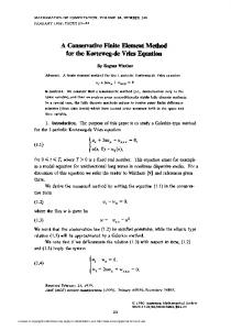
φe1 (x 1, y 1) y
1
x Element e P(x, y) 2 3
(x2, y 2) φe2
(x 3, y 3) φ e3
Fig. 1
A typical first order triangular element.
Triangles with fe expressed as linear functions are called first-order triangular elements. Fig. 1 shows a triangle where the values of coordinates and fe at the vertices are shown. Using the linear approximation in eqn (4), we can write f e1 = a + bx1 + cy1 f e 2 = a + bx 2 + cy2
f e 3 = a + bx3 + cy3 .
Solution of these equations gives 3
a = ∑ aif ei i =1
3
b = ∑ bif ei i =1
3
c = ∑ cif ei i =1
where, ai = (xi1yi2 − xi2yi1)/(2Ae), bi = (yi1 − yi2)/(2Ae), and ci = (xi2 − xi1)/(2Ae). i, i1 and i2 are a cyclic permutation of 1, 2 and 3. Hence, we can write 3
f e = ∑ uif ei i =1
where the terms ui = ai + bix + ciy are also known as barycentric or area coordinates. It may be noted that 3 ∂f e = ∑ bif ei ∂x i =1
and
3 ∂f e = ∑ cif ei . ∂y i =1
Using row vectors fe = [fe1 fe2 fe3], u = [u1 u2 u3], b = [b1 b2 b3] and c = [c1 c2 c3], (3) can be written as F(f ) =
t t 1 Ne (bf et ) bf et + (cf et ) ∑ cf t − k 2(uf t )t uf t ds 2 e=1 ∫∫ e e e Ae
where the superscript t indicates the transpose. Hence, F(f ) =
1 Ne ∑ {fe Pefet − k 2fe Qefet } 2 e=1
International Journal of Electrical Engineering Education 43/3
(5)
FEM in electromagnetics using MATLAB
235
where, Pe = Ae{b t b + c tc}
(6)
and Qe =
2 1 1 Ae 1 2 1 . 12 1 1 2
(7)
To obtain the matrix Qe, one uses the result provided in Ref. 8:
∫∫ u u
u ds =
l m n 1 2 3
Ae
l! m! n! 2! Ae . (l + m + n + 2)!
Matrices with subscript e, obtained for triangle number e, are called local matrices. Forming local matrices with MATLAB The first step in the FEM is to generate a triangular mesh over the cross-section, S. As mesh generation is not the object of this introductory paper, there are several options: (i) download free mesh generator programs from the internet; (ii) use mesh generators of any available FEM software (e.g., civil engineering FEM software); and (iii) use pdetool available in MATLAB. For simplicity, only one domain (region) with one boundary and first-order triangular elements will be considered. Most mesh generators produce text files as output which can be edited to yield the following data: Triangle node numbers A file element.txt which has three columns containing three node numbers of each triangle, with rows arranged to correspond to triangle numbers in ascending order. Coordinates of nodes A file coord.txt which has two columns containing x coordinate in the first column and y coordinate in the second, with rows arranged to correspond to node numbers in ascending order. Boundary node numbers A file bn.txt with one column containing the boundary node numbers in ascending order. The function M-file triangle.m contains the following MATLAB program to compute the local matrices Pe and Qe. International Journal of Electrical Engineering Education 43/3
236
M. K. Haldar
function [pe,qe] = triangle (x,y) ae=x(2)*y(3)-x(3)*y(2)+x(3)*y(1)x(1)*y(3)+. . . x(1)*y(2-x(2)*y(1); ae=abs(ae)/2; b=[y(2)-y(3),y(3)-y(1),y(1)-y(2)]; c=[x(3)-x(2),x(1)-x(3),x(2)-x(1)]; b=b/(2*ae); c=c/(2*ae); pe=(b.’*b+c.’*c)*ae; qe=[2,1,1;1,2,1;1,1,2];qe=qe*(ae/12);
Forming global matrices with MATLAB If the total number of nodes is Nn, eqn (5) can be written as F(f ) =
1 Ne ∑ { fPegf t − k 2f Qegf t } 2 e=1
(8)
where f = [f1 f2 . . . fNn], and P eg and Qeg are Nn × Nn square matrices, such that if p, q and r are node numbers (1), (2) and (3) of triangle e, only nine matrix elements of Peg and Qeg are nonzero: pp, pq, pr, qp, qq, qr, rp, rq and rr. Equation (8) can be written as: F(f ) =
1 [f P gf t − k 2f Q gf t ] 2 Ne
Ne
e =1
e =1
(9)
where P g = ∑ P eg and Q g = ∑ Qeg . Pg and Qg are called global matrices. The global matrices are thus obtained by adding the local matrices written as Nn × Nn square matrices. This operation is easily carried out by the following MATLAB program (explained by comments following %).
% load the data files load element.txt; load coord.txt; load bn.txt; % Find the total number of elements and nodes ne=length(element(:,1)); nn=length(coord(:,1)); % Set up null global matrices pg=zeros(nn,nn); qg=zeros(nn,nn); % Sum over all triangles International Journal of Electrical Engineering Education 43/3
FEM in electromagnetics using MATLAB
237
for e=1:ne; % Get the three node numbers of triangle number e node=[element(e,:)]; % Get the coordinates of each node and form row vectors x=[coord(node(1),1),coord(node(2),1),coord(node(3), 1)]; y=[coord(node(1),2),coord(node(2),2),coord(node(3), 2)]; % Calculate the local matrix for triangle number e [pe,qe]=triangle(x,y); % Add each element of the local matrix to % the appropriate element of the global matrix for k=1:3;for m=1:3; pg(node(k),node(m))=pg(node(k),node(m))+pe(k,m); qg(node(k),node(m))=qg(node(k),node(m))+qe(k,m); % Close the three for loops end;end;end;
Forming the FEM equations The functional given by eqn (9) can be written as F(f ) =
1 Nn Nn g 1 Nn Nn f i ∑ Pijf j − k 2∑ f i ∑ Q ijgf j ∑ 2 i =1 j =1 2 i =1 j =1
(10)
The finite element solution is obtained by minimising the functional in (10) with respect to the nodal values, i.e., by setting ∂ F(f ) = 0 for k = 1, 2, . . . Nn . ∂f k Thus 1 Nn g 1 Nn Pik + Pkig )f i − k 2 ∑ (Q ikg + Q gki )fi = 0. ( ∑ 2 i =1 2 i =1 Since the matrices are symmetrical, this becomes Nn
Nn
i =1
i =1
∑ Pikgfi − k 2 ∑ Qikgfi = 0 or in matrix form, P gf t − k 2 Q gf t = 0.
(11)
Now one has to implement boundary conditions. Only perfectly conducting boundaries are considered here. The number of boundary nodes is denoted as Nb. International Journal of Electrical Engineering Education 43/3
238
M. K. Haldar
Boundary conditions: TE modes For TE modes, f represents the axial magnetic field, Hz, and the boundary condition is the Neuman condition, df/dn = 0, where n is the normal to the perfectly conducting boundary. In FEM, this is a natural boundary condition and need not be imposed. Thus the values at the boundary are considered to be unknown and the eigenvalue equation (11) is solved using the MATLAB statement ksquare = eig(pg,qg). Boundary conditions: TM modes For TM modes, f represents the axial electric field, Ez, and the boundary condition for the perfectly conducting boundary is, f = 0. This is the Dirichlet condition, which must be strictly imposed in the FEM. It requires the following: (i)
Omitting differentiation with respect to the known boundary nodes. This can be done by simply deleting the rows of Pg and Qg corresponding to the boundary nodes. (ii) Deleting the columns of Pg and Qg corresponding to the boundary nodes, as f = 0 at these nodes. The deletion of the row and column corresponding to a boundary node is easily accomplished using Matlab’s dynamic memory allocation feature. The deletion procedure is implemented as follows:
% Find the total number of boundary nodes,nb nb=length(bn(:,1)); % Create an auxiliary column vector of % boundary nodes bnaux=bn; for n=1:nb; %Read the node number k of the boundary node k=bnaux(n); % Delete kth row and column of the global % matrices pg(k,:)=[]; qg(k,:)=[]; pg(:,k)=[]; qg(:,k)=[]; % After deletion, the row/column numbers % corresponding to boundary node numbers>k are % reduced by one. As boundary node numbers are % in ascending order, all node numbers can be % reduced with a unit column vector of length nb bnaux=bnaux – ones(nb,1); end; International Journal of Electrical Engineering Education 43/3
FEM in electromagnetics using MATLAB
239
As before, the eigenvalue equation is solved, but this time with the reduced matrices obtained with the above procedure. Homogeneous hollow waveguide examples There are many homogeneous hollow waveguide problems in the available literature which can be given as assignments to students. Four examples are given here. In these examples, pdetools was used to get first-order triangular mesh data. All the examples can be worked out with notebook PCs. Homogeneous rectangular waveguide The waveguide (WR-90) dimensions are 2.286 × 1.016 cm. Tables 1 and 2 compare the FEM and analytical values of k2 for TEmn and TMmn modes respectively. m represents the number of half wavelengths along the longer side and n represents the number of half wavelengths along the shorter side. FEM values are obtained with 2688 triangles and 1405 nodes. It may be seen that the error increases for higher values of k2, i.e., for higher-order modes. This is because for a given triangle size, the linear approximation inside a triangle can better represent f for lower-order modes which vary less rapidly in the waveguide cross-section. Homogeneous square waveguide This example is used to show degenerate (equal) eigenvalues. It also allows one to progress towards a physical understanding of why FEM produces degenerate eigenvalues for circular waveguides. The waveguide dimensions are 1.5 × 1.5 cm. For the sake of brevity, a comparison of FEM and analytical results is shown only for TE modes in Table 3. FEM values are obtained for 4960 triangles and 2565 nodes. It may be seen that modes such as TE12 and TE21 have the same eigenvalue. It is noted that rotating the field profile of the TE12 mode by 90° gives the field profile of the TE21 mode. TABLE 1 m
n
0 1 2
TABLE 2 m 1 2 3
n
Values of k2 (in cm−2) for TEmn modes (analytical values in brackets) 0
1
2
No mode 1.889(1.889) 7.563(7.555)
9.574(9.561) 11.468(11.450) 17.157(17.116)
38.459(38.245) 40.366(40.133) 46.104(45.799)
Values of k2 (in cm−2) for TMmn modes (analytical values in brackets) 1
2
3
11.468(11.450) 17.158(17.116) 26.662(26.559)
40.362(40.133) 46.103(45.799) 55.695(55.242)
89.024(87.939) 94.846(93.605) 103.655(103.048)
International Journal of Electrical Engineering Education 43/3
240
M. K. Haldar
TABLE 3 m
n
0 1 2
TABLE 4 m 0 1 2
n
Values of k2 (in cm−2) for TEmn modes (analytical values in brackets) 0
1
2
No mode 4.388(4.386) 17.569(17.546)
4.388(4.386) 8.778(8.773) 21.967(21.932)
17.567(17.546) 21.967(21.932) 35.184(35.092)
Values of k2 (in cm−2) for TEmn modes (analytical values in brackets) 1
2
3
6.540(6.526) 1.507(1.506) 4.151(4.146)
22.013(21.877) 12.681(12.631) 20.102(19.987)
46.581(46.005) 32.684(32.384) 44.289(44.178)
Homogeneous circular waveguide The radius of the circular waveguide is taken as 1.5 cm. FEM and analytical values of k2 for TEmn modes are given in Table 4. m represents the degree of rotational symmetry of the fields and n represents the nth root of the characteristic equation for k. FEM values are obtained for 4160 triangles and 2145 nodes. For m ≠ 0, the FEM produces two equal eigenvalues. As in the square waveguide, the field patterns corresponding to these equal eigenvalues are rotated by 90° with respect to one another. For m = 0, rotation by 90° produces identical patterns. This result is not obvious from analytical methods. Design example: single ridge waveguide Design curves for single ridge waveguides were obtained analytically by Hopfer.14 Figs 2 and 3 compare the FEM solutions, represented by dots, with some of the design curves given in Figs 5 and 7 of Hopfer’s paper respectively. Good agreement is obtained. Moreover, Fig. 3 illustrates the power of the FEM. In the range, 0.008 < s / a < 0.50, Hopfer was unable to obtain analytical solutions using a single rectangular waveguide TE mode as the TE30 mode cannot exist by itself but couples to the TE01 mode. The FEM analysis has no such limitation. It must be mentioned that for all the waveguide examples considered, a very small eigenvalue for TE modes was produced by FEM. This value approximates the zero eigenvalue corresponding to the f = constant mode15 and is ignored. Extension to other problems In this section, it is shown that the discussion in Section II can with minor extensions be used to solve many other problems. For the sake of brevity, we consider only two of them. International Journal of Electrical Engineering Education 43/3
FEM in electromagnetics using MATLAB
241
Fig. 2
Single ridge waveguide TE10 mode cut-off wavelength a = 2.286 cm and b/a = 0.45. Dots represent values calculated by FEM.
Fig. 3
Single ridge waveguide TE30 mode cut-off wavelength a = 2.286 cm and b/a = 0.45. Dots represent values calculated by FEM.
International Journal of Electrical Engineering Education 43/3
242
M. K. Haldar
Electrostatic problems The functional for Laplace’s equation is: F(f ) =
∂f 2 ∂f 2 1 e e + 0 r ds 2 ∫∫ ∂ x ∂ y S
where f represents the electric potential. e0 is the permittivity of free space and er is the dielectric constant. For homogeneous isotropic media, it is easy to see that the FEM equation is Pgf t = 0, the matrix P g being the same as that in Section II.D. Two boundaries are considered here. The mesh data should have two sets of boundary nodes. We can take f = 0 at one boundary. For nodes on this boundary, the corresponding rows and columns of P g are deleted. For the other boundary, f = V, a numerical value. The rows of P g corresponding to nodes on this boundary are deleted as before. However the column corresponding to each node is multiplied by −V and put as a separate matrix. The matrices are added together to form the matrix R. Next the columns are deleted from P g to get the reduced matrix P. The FEM equation is now of the form Pf t = R which can be solved for f t using Matlab. Wave propagation in inhomogeneous waveguides For homogeneous waveguides, the refractive index, n, is constant and so k is a constant. We could find the eigenvalue k2 and then compute the propagation constant, kz, from k 2z = erk20 − k2 and k0 = 2p/l0 for a given wavelength, l0. For an inhomogeneous waveguide, eqn (8) is written as: 1 Ne ∑ {fPeg f t − e re k02fQeg f t + kz2fQeg f t } , where, ere is the relative permit2 e=1 tivity of the medium inside element number e. Hence eqn (9) becomes: F(f ) =
F(f ) =
1 1 f R gf t − kz2f Q gf t 2 2
(12)
where g 2p 2 R = ∑ P e − e re Q eg l 0 e =1 and Ne
g
Ne
Q g = − ∑ Q eg . e =1
Equation (11) now becomes R gf t − kz2 Q gf t = 0.
(13)
The only modification is to generate the mesh with elements of different relative permittivity, ere, and find Rg for a given wavelength, l0. Unlike for a homogeneous International Journal of Electrical Engineering Education 43/3
FEM in electromagnetics using MATLAB
243
waveguide we need to determine the eigenvalue, kz2, numerically for each wavelength. Conclusion It is shown how the FEM can be introduced to electrical engineering undergraduates using only a few lines of MATLAB code. The MATLAB codes relate directly to the FEM operations. Four waveguide examples are given. These examples can be run on a standard PC. A design example illustrated the advantage of FEM compared to an analytical method. It was also shown how the concepts acquired can be readily extended to other problems. The demonstrated problems are 2D in nature. However, similar programming techniques can be employed for more complex problems, such as 3D problems presented, for example, by Silvester and Ferrari.6 Institutions with inadequate financial resources may benefit from the proposed methodology, as only MATLAB is needed, no add-ons (not even a mesh generator). The material presented in this paper may also be useful to beginning research students who are uninitiated in the FEM. Acknowledgement The author thanks Mr Duen Hong Ong, an undergraduate, for the results given in Section III.
References 1
2 3 4 5 6 7 8 9 10 11 12
J. Lu and D. V. Thiel, ‘Computational and visual electromagnetics using an integrated programming language for undergraduate engineering students’, IEEE Trans. Magnetics, 36 (2000), 1000–1003. S. Selleri, ‘A Matlab experimental framework for electromagnetic education’, IEEE Antennas and Propagat. Mag., 45 (2003), 85–90. S. Selleri, ‘A Matlab application programmer interface for educational electromagnetics’ in Antennas and Propagat. Soc. Symp, 22–27 June, 2003. S. Makarov, ‘MoM antenna simulations with Matlab RWG basis functions’, IEEE Antennas and Propagat. Mag., 43 (2001), 100–107. MATLAB, The Math Works Inc., http://www.mathworks.com P. P. Silvester and R. L. Ferrari, Finite Elements for Electrical Engineers (Cambridge University Press, Cambridge, 1990). J. Jin, The Finite Element Method in Electromagnetics (John Wiley and Sons, New York, 1993). S. R. H. Hoole, Computer-Aided Design of Electromagnetic Devices (Elsevier, New York, 1989). T. Itoh, G. Pelosi and P. P. Silvester, Finite Element Software for Microwave Engineering (John Wiley and Sons, New York, 1996). K. Foster, ‘Retaking the field – an old computational favourite is overhauled’, IEEE Spectrum, July (2004), 54–55. L. Y. Tio, A. A. P. Gibson, B. M. Dillon and L. E. Davis, ‘Weak form finite element formulation for Helmholtz equation’, Int. J. Elect. Enging. Educ., 41 (2004), 1–9. S. Ramo, J. R. Whinnery and T. Van Duzer, Fields and Waves in Communication Electronics (John Wiley, New York, 1994). International Journal of Electrical Engineering Education 43/3
244
M. K. Haldar
13 A. K. Ghatak and K. Thyagarajan, Optical Electronics (Cambridge University Press, Cambridge, 1989). 14 S. Hopfer, ‘Design of ridged waveguides’, IRE Trans. Microw. Theory. Tech., 3 (1955), 20–29. 15 P. Silvester, ‘A general high-order finite element waveguide analysis program’, IEEE Trans. Microw. Theory Tech., 17 (1969), 204–210.
International Journal of Electrical Engineering Education 43/3