Hierarchical clustering and filtering in half-inverse ... - Semantic Scholar

350

IEEE TRANSACTIONS ON SIGNAL PROCESSING, VOL. 51, NO. 2, FEBRUARY 2003

Hierarchical Clustering and Filtering in Half-Inverse Space for MEG and/or EEG Hypothesis-Free Analysis Ayumu Matani, Member, IEEE, Yasushi Masuda, Member, IEEE, Hideaki Okubo, and Kunihiro Chihara, Member, IEEE

Abstract—We propose hierarchical clustering and filtering methods for the analysis of spatio–temporal multidimensional time series, where both methods are based on a new pseudo distance. The pseudo distance is determined between orthogonal matrices, which are derived by eigenvalue decomposition of the variance–covariance matrix of the time series. Because the grouping algorithm is also important in clustering, a modified Ward method grouping criterion is used here. The filtering derives temporal similarity information between two time series, providing information that cannot be evaluated by the clustering. If the time series to be clustered and filtered cannot be obtained directly, different time series reflecting the original time series are used instead. There exists a transform between the time series, and hence, scaling distortion occurs. We also propose a scaling normalization method. As an application example, we present an analysis of a multichannel magnetoencephalography (MEG) and/or electroencephalography (EEG) time series. Each of the MEG and EEG generations is a transform from the same electrophysiological brain activity. We applied these methods to sound localization-related MEG time series and evaluated their effectiveness. These methods may be useful for discovering similarity among many multidimensional time series without a priori information and/or hypotheses. Index Terms—Electroencephalography (EEG), filtering, hierarchical clustering, hypothesis-free, magnetoencephalography (MEG), normalization, sound localization, spatio–temporal multidimensional time series.

I. INTRODUCTION

C

LUSTERING methods are classified into two classes, namely, hierarchical and nonhierarchical [1]. Hierarchical clustering is appropriate for analysis without a priori knowledge of the data sets to be clustered, and hence, hierarchical clustering is often categorized in unsupervised learning. If many data units are prepared and then are clustered to find within-cluster characteristics, hierarchical clustering is a powerful tool. In practice, hierarchical clustering consists of Manuscript received September 14, 2001; revised September 24, 2002. This work was supported in part by Core Research Evolutional Science and Technology (CREST) of Japan Science and Technology Corporation (JST). The associate editor coordinating the review of this paper and approving it for publication was Dr. Alex B. Gershman. A. Matani is with the Graduate School of Frontier Sciences, the University of Tokyo, Tokyo, Japan (e-mail: [email protected]). Y. Masuda is with the Department of Gerontechnology, National Institute for Longevity Sciences, Aichi, Japan (e-mail: [email protected]). H. Okubo is with the Core Technology and Network Company, SONY Corporation, Tokyo, Japan (e-mail: [email protected]). K. Chihara is with the Graduate School of Information Science, Nara Institute of Science and Technology, Nara, Japan (e-mail: [email protected]). Digital Object Identifier 10.1109/TSP.2002.806978

two steps: i) calculation of distances between all pairs of data units; ii) hierarchical grouping. In this paper, we limit data units to spatio–temporal multidimensional time series from spatially location-fixed multichannel recorded time series. Each multidimensional time series is represented by a matrix (column: spatial pattern, row: temporal activity). A distance appropriate for evaluating the dissimilarity in the nature of the recording is then chosen, or is determined, between the matrices. Let us assume there two matrices and and take some examples of the distance, which satisfy the distance axiom between the matrices. The Frobenius norm tr simply denotes the Euclidean distance by . The square for all of the elements of is also root of the largest eigenvalue of sometimes used. Those distances based on the difference are intuitive but are occasionally even sensitive to and in terms of the nonintrinsic differences between nature of the recording. Apart from the choice of distance, grouping algorithms are approximately classified into two, namely, merging two clusters having the nearest distance and merging two having the smallest approximation errors. In the former, there are further two extreme determinations of distance between clusters, namely, the nearest distance between data units from one cluster to another (single linkage) and the furthest distance (complete linkage) [1]. The former, with the two extreme determinations, is indifferent to the approximation error of each generating cluster. If something central in a cluster is treated as the representative of the cluster, the approximation error is produced by the representation. Taking the approximation error into account, the latter is proposed. The Ward method [2] with its fast algorithm [3] is a typical example. The grouping criterion is to find the minimum increment of the approximation error by merging. Details of the Ward method will be explained in Section II-B; the Ward method does not simply merge the nearest as the single and complete linkages and works only with the Euclidean distance. On the other hand, in nonhierarchical clustering, one first determines the number of clusters [1]. The determination requires a priori knowledge of the data units to be clustered. The -means method [4] is a typical example for generating clusters. After determining , the -means method performs as follows. i) initial centroids are determined. ii) Each data unit is classified with the nearest centroid. iii) The centroid of each cluster is recalculated.

1053-587X/03$17.00 © 2003 IEEE

MATANI et al.: HIERARCHICAL CLUSTERING AND FILTERING IN HALF-INVERSE SPACE

The second and third steps are iterated until the change of centroids is sufficiently small. For example, speech recognition is often performed as a nonhierarchical clustering of multidimensional time series. Speech is treated as a frequency pattern (vector) time series. Clustering of vector patterns such as speech recognition is called vector quantization [5]. In practice, vector quantization consists of two steps: i) determination of a representative of each cluster (codevector) by supervised learning from training data units; ii) classification of the other data units into one of the clusters. In the first step, the LBG algorithm [6], or the Lloyd algorithm [7], is widely used. The LBG algorithm is very similar to the -means method in the iteration procedure. The Pairwise Nearest Neighbor (PNN) algorithm [8] was proposed as an alternative to the LBG algorithm. It has been pointed out that the PNN algorithm is identical to the Ward method [9]. Regarding grouping algorithms, even in nonhierarchical clustering, the importance of the Ward method is seen in a new light. Although hierarchical clustering clarifies the similarity between multidimensional time series, it cannot evaluate temporal similarity information between two multidimensional time seand are the th column vectors of ries. Assume that and , respectively, where denotes the th the matrices ( ) and time sampling point. If the similarity between ( ) is calculated, then the temporal similarity information can be evaluated. This may be achieved by a filtering to extract ( ). the characteristics of ( ) from Let us limit the spatially location-fixed multichannel recording data to magnetoencephalography (MEG) and/or electroencephalography (EEG) time series. There are some application examples of clustering in EEG time series. Nonhierarchical clustering is often used for classifying specific waveforms [10], [11] and for selective averaging [12], [13]. However, we have not found previous studies concerning hierarchical clustering applied to MEG and/or EEG time series. Usually, brain researchers have a priori information of the recorded MEG and/or EEG time series or hypotheses about brain functions of interest, and hence, they can set the number of clusters and/or the representative of each cluster. This situation fits for nonhierarchical (also often supervised) clustering rather than hierarchical unsupervised clustering. Conversely, if brain researchers do not have any a priori information and/or hypotheses, then their standpoint is hypothesis-free. For those with a hypothesis-free standpoint, a strategy to develop hypotheses is that they record many numbers of MEG and/or EEG time series under different conditions and then perform hierarchical unsupervised clustering. The result may suggest a new hypothesis. In this paper, we propose hierarchical clustering and filtering methods, both of which are based on a newly determined pseudo distance between multidimensional time series. As an example, these methods are applied to sound localization-related MEG time series.

351

first three subsections and then explain the normalization method in an application to MEG and/or EEG in the last subsection. A. Distance A spatially -dimensional and temporarily ries is obtained as

-point time se(1) (2)

s have a sufficiently high signal-toLet us assume that noise ratio (SNR) and are well highpass filtered to be mean zero , where signals. Then, the eigenvalue decomposition of reflects the variance–covariance matrix of in the time average sense, is performed as

(3) where diag

(4) (5) (6)

diag

(7)

diag

(8) (9) (10)

and are the th eigenvalue and In (4) and (6), eigenvector (unit vector), respectively. The eigenvalues are in (5) plays placed in descending order as shown in (5). the role of the partition number dividing the large and small s, where are relatively large eigenvalues, namely, are relatively small. The subscripts and those where “ ” and “ ” in (7)–(10) denote large and small in the above sense. The subscript “ ” indicates the multidimensional time of (1) and of (2). Since has a relatively high series SNR, one may divide the signal and noise subspaces of by and [both in (3)]. Such a division procedure is popular in multiple signal classification (MUSIC) [14]–[16]. is determined empirically or by noise The partition number , level, as in MUSIC. Let us determine three operators , and , all of which extract the matrices from the matrices in the parentheses, corresponding to (6), , (9), and (10), respectively. For example, , and can be realized. The operators are used throughout this paper. Now, assume another multidimensional time series having the same size of as

II. METHODS We explain the clustering and filtering methods applied to general spatio–temporal multidimensional time series in the

(11) (12)

352


and s also have a high SNR and are mean zero signals. We then have

. If one needs sensitivity to temporal characteristic, then inone should start from the eigenvalue decomposition of stead.

(13) B. Grouping (14) in (3) and Both and both orthogonal matrix to be

of (13) are orthogonal matrices because are symmetric matrices. Therefore, the for the transform of to is found

(15) . assuming that the same partition number can be used for ( ) is the coefficient matrix partially In (15), ( ) by ( ). A norm of spanning ( ) therefore expresses the similarity between the signal ( ) and the noise subspace of ( ). It also subspace of expresses the dissimilarity between the signal subspaces of and . If the Frobenius norm is employed here, then the proposed distance between and (16) , is determined. The proposed distance (16) ranges from 0 to and which is shown by the following reasoning. If are orthonormal complements with respect to each other, then , so that . [It is a proof of (17).] is completely a part of the If, on the contrary, the span of , then . Although this also requires span , it is empirically true in almost every case for actual recorded multidimensional time series having relatively large because of the redundancy of the recording. In dimension another important feature of the proposed distance, the distance satisfies the pseudo distance axiom

The Ward method [2] is often used for hierarchical clustering and is characterized by the following two properties. i) It works with the Euclidean distance. ii) It employs a grouping algorithm for minimizing the cost function determined by the increment of the sum of the squared Euclidian distances of within-cluster data units from their centroid. The centroid is simply calculated as an arithmetical mean. The square sum plays the role of the approximation error if the centroid is treated as the representative of the within-cluster data units. In general, the centroid is characterized by the point minimizing the approximation error (second-order moment). This characteristic implicitly relates to the fast algorithm [3] of the Ward method. However, during the procedure to calculate the proposed distance (16), the information regarding the original multidimensional time series of (1) remains only in the orthogonal matrix in (3) and the partition number in (5). A problem therefore arises from the direct application of the proposed distance instead of the Euclidian distance to the Ward method. We must prepare something as a substitute for the centroid as used in the Ward method. Since the data units here are orthogonal matrices, a natural extension is that the substitute for the centroid should be an orthogonal matrix. However, the arithmetic mean of orthogonal matrices cannot be an orthogonal matrix. Now, assume s, that multidimensional time series exist in the th cluster . Set the centroid as an orthogonal matrix

where the number of columns of is and is the same partition number in (5). In this case, we calculate the approximation error from the substitute centroid in the same manner as represented by (16). Thus, the approximation error should be expressed by (20)

(17) (18)

Let us keep the same characteristic so that the centroid minimizes approximation error. Therefore

(19) where proofs of (18) and (19) can be found in Appendix A. Symmetry property (18) supports the last equals sign of (16). To put it simply, the proposed distance is a norm of the projection of the signal subspace of a data unit to noise subspace of another data unit and, hence, is based on the subspace method [17] or principal component analysis (PCA). The proposed distance (16) is sensitive to spatial characteristic because it is derived from the eigenvalue decomposition of

tr

tr


is achieved if the columns of span the space through s are distributed as poorly as poswhich the columns of sible. Therefore (21) , but this is Of course, is required to calculate the unimportant because only approximation error (20), and the two spaces spanned by the and are orthogonal complements with columns of respect to each other. Let us now return to the grouping algorithm. Assume that the number of multidimensional time series is . The proposed grouping algorithm based on the Ward method is expressed as follows. Stage 1) Begin with clusters, each of which consists of one multidimensional time series. At this stage, the approximation error is zero. Stage 2) At each stage, reduce the number of clusters by by comone through generating a new cluster and , whose combinabining two clusters tion produces the smallest increment of the approximation error using (20) and (21). times until the number Stage 3) Continue Stage 2 of clusters is one. C. Filtering First, the multidimensional time series tracted and is whitened to be

of (2) is con(22)

is zero mean, exists in the span of [in (3)] Since and has, by whitening (22), unit variance for any direction in the span. Second, with (22) and (14), the proposed distance (16) is represented by another form (23) where (24) of (24) is a filtering The proof is found in Appendix B. that is dissimilar to that indicates temporal information of of (11). Finally, the inversion filtering of (24) (25) that is similar to . indicates the temporal information of Such an inversion filtering is popular in array signal processing , the [18]. We call , which produces the Gram matrix target of the filtering. The filtering measures the characteristic of is the target in a multidimensional time series. Note that , which is used for evaluating of (12) not equal to

353

similar to of (1) because ( ) is not the only multi( ) and that dimensional time series to generate ( ) is invariant to ’s permutation of ( ). At this stage, we have explained the filtering as an analyzing method for evaluating the contribution between two multidimensional time series. It is also useful for evaluating the contribution within a multidimensional time series, between a partial multidimensional time series for one specific time duration and that for another time duration. In MEG time series analysis, there are two methods similar to the filtering (25), namely, MUSIC [15], [16] and signal space projection (SSP) [19]. In the mathematical form of the filtering . The filtering (25), MUSIC has the same Gram matrix projects another MEG and/or EEG time series to the Gram matrix, whereas MUSIC projects MEG generation model (leadfield vector; see Section II-D) to that. In normalization of the different projecting terms explained above, the filtering employs whitening (22), whereas MUSIC employs division by norm. The filtering does not require the MEG and/or EEG generation model, and thereby, it is a nonparametric metric. The other method (SSP) is occasionally a nonparametric metric. In SSP, first, some feature MEG vectors (spatial patterns) are prepared, and they are treated as bases which span the feature MEG space. Another MEG time series is then projected to one of the dual bases. If the feature MEG vectors are selected from a MEG time series and another MEG time series is projected to the space spanned by the feature MEG vectors, then SSP can evaluate the similarity between them in the meaning of the selected feature MEG vector. A difference between the filtering and SSP is that the filtering is a projection to a matrix, whereas SSP is a projection to a vector. D. Scaling Normalization for MEG and/or EEG Activity An often encountered difficulty is to obtain directly the spatio–temporal multidimensional time series to be clustered and filtered. In this case, different time series reflecting the time series may be used instead. There exists scaling distortion between these two time series. Even if the reflection is expressed by a mathematical transform, the transform is a forward model and is often difficult to invert. The transform is usually nonlinear but is often approximated by a linear system equation by spatial discretization [20]. The linear approximation can clarify the problem of inversion. In this subsection, we propose a scaling normalization method. No matter which general case fits for the above situation, the normalization method can be applied. However, since discussion of both the general case and the specific case of MEG and/or EEG is somewhat redundant, here, we explain the specific case only. If the proposed clustering and filtering methods are used for brain signal processing, the most appropriate multidimensional time series to be analyzed may be the electrophysiological brain activity because the electrophysiological brain activity is a primary representation of inside and outside brain phenomena. Since the direct detection of the activity using inserted needle electrodes is invasive, such detection is impossible in brain studies using volunteer subjects. MEG and/or EEG may be used instead since both MEG and EEG are generated by the same source: the electrophysiological brain activity. In mathematical

354


models of the brain, the electrophysiological brain activity is usually approximated by current dipoles [21]. There exists a transform model from the current dipole to the MEG and/or EEG as follows. First, the current dipoles, as a vector field, are represented by fixed orientation vectors on spatially discretized (grid grids in the brain volume. If the number of grids is ), then the number of parameters of the index: (dipole index: ) current dipoles will be in three-dimensional (3-D) space. Note that the current dipoles are located at the same indexed by grid. In addition, if the number of time samples is , then the current dipoles’ activity time series are denoted by in matrix form

Second, generates the MEG and EEG time series , and the numbers of detectors are and respectively, as

and ,

(33)

where all subscripts indicated by “ ” are replaced by subscript either “MEG” or “EEG.” Finally, we can represent the transform as a linear system equation (26) and where and EEG, respectively

respectively. in (31) is the th singular value of in and in (32) are the identity (28). zero matrix, respectively. Let matrix and the of (29) step by step. us discuss the inverse procedure using is rotated by . Second, the scaling First, the time series . In this step, the of the rotated time series is changed by first problem occurs in that the inverse numbers of the relatively small singular values occasionally amplify the noise additive to . The transform generated by is labeled here as the half-inverse transform, and the transformed space is labeled the half-inverse space. The dimension of the half-inverse space is . Third, the half-inverse transformed time series is instill -dimensional space by . In this step, the second serted in problem occurs; it is caused by the underdeterminedness. Fi. Note that the nally, the processed time series is rotated by first and second problems are independent with respect to each other. The scaling normalization is therefore achieved by the half-inverse transform

are the leadfield matrices of the MEG (27)

is the In the leadfield matrix (27), the leadfield vector MEG or EEG spatial pattern, produced by the th current dipole having unit magnitude. For detailed calculation of the leadfield vector, see [22]–[24] for MEG and [22], [25], and [26] for EEG. Let us use (28) for addressing to either MEG or EEG. The ill conditioning of to ) in (28) is mainly caused by unthe inverse transform ( ). Therefore, although the unique derdeterminedness ( solution cannot be obtained, the Moor—Penrose pseudo inverse for achieving the minimum norm solution is expressed by

(in the half-inverse space) is The scaling in the space of equal to the space of , except for the kernel of the transform (28). Apart from that, regularization may be necessary for in (33) to overcome the first problem. However, we are not concerned here with regularization because it has been well investigated [20], and accordingly, its implementation is not difficult. The half-inverse transform (33) is applied to and [both in (26)] separately, and therefore, and are obtained. Then, the hierarchical clustering and the filtering can be applied to the appended matrix [left-hand-side term of (26)]. By the way, optionally, the transform (33) is replaced by to maintain the characteristic of each is in the MEG and/or EEG detector. The additional term in whitening (22). charge of the maintenance like the term Whichever definition is selected as the half-inverse transform, no difference occurs to the hierarchical clustering and the is an orthogonal matrix, and hence, it just filtering because effects rotation. The half-inverse transform is useful for the scaling normalization, not only between the current dipole and either MEG or EEG, but between MEG and EEG as well. Although whitening is a scaling normalization method, it is nonparametric and, hence, is not appropriate for this scaling normalization, which takes the MEG and/or EEG generation model into account. III. EXPERIMENTS

(29) A. MEG Recording where the singular value decomposition of

is (30)

diag

(31) (32)

and in (30) are orthogonal matrices whose columns span the MEG activity space and the current dipoles’ activity space,

We performed MEG experiments to evaluate the hierarchical clustering and the filtering in the half-inverse space. As a test example, we adopted sound localization-related MEG. Sound localization is a human perception by which one can localize a sound source. In general, interaural intensity difference (IID) [27], [28] and interaural time difference (ITD) [29]–[31] play important roles in sound localization. The subject, hearing an IID or ITD stimulus through headphones, recognizes a virtual


355

TABLE I SOUND LOCALIZATION EXPERIMENTS WITH INTERAURAL TIME DIFFERENCE (ITD) STIMULI

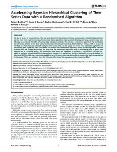
Fig. 1. Interaural time difference (ITD) stimuli. (a) Continuous click trains are presented to both ears of the subject. (b) Hearing the stimulus through headphones, the subject recognizes the sound image in the head. (States; C: center, LS: left small, LL: left large, RS: right small, RL: right large, S: silence).

sound source in the head. The virtual sound source is often called the sound image. In this study, we used only ITD stimuli comprising continuous click trains [32], as shown in Fig. 1(a). We set the pulse width and the interval to 454 s and 14.3 ms, respectively. The states of the sound images at the center (C), left small (LS), left large (LL), right small (RS), and right large (RL), as shown in Fig. 1(b), were set with the offset to 0, 385, 680, 385, and 680 s, respectively. In addition to the states of the sound images, the state of the silence (S) was also prepared. Actually, the stimuli consisted of changes from one state to another. To support the hypothesis-free standpoint, since many types of stimuli should be prepared, we performed all permutations of the states accordingly, as shown in Table I. Consequently, a total of 30 types of stimuli were prepared. The stimuli, including the state S, were used for the sudden appearance of the sound image (type onset) or for its sudden disappearance (type offset). The other stimuli were used for the shift of the sound image (type shift, further divided into types left-shift and right-shift by their shift direction). To avoid or to reduce prediction and habituation of the subject repeatedly hearing the stimuli, the lengths of the states were randomly changed (1–1.5 s), and the same types of stimuli were randomly presented 50 times per type. The MEG time series corresponding to all of the stimuli were recorded with a 64-channel whole-head biomagnetometer (CTF Systems Inc., Canada) installed in a magnetically shielded room (Tokin Corp., Japan). The recordings were performed under the same conditions, where the sampling frequency and pre- and post-trigger recording durations were 1250 Hz, and 100 and 500 ms, respectively. After the recordings, the same types of MEG time series were averaged together and were bandpass filtered

(1–40 Hz). We did not simultaneously record EEG due to an interference problem caused by a mismatch between the MEG and the EEG detecting systems we attempted to use. B. Analysis in (26) was first determined, The leadfield matrix where a sphere having homogeneous conductivity [24] was employed for the MEG generation model. Since this spherical model required the location of the center of the sphere, this was determined by least squares fitting of the brain surface of the magnetic resonance imaging (MRI) volume data of the subject [33]. One of the most important characteristics of the spherical model is that the current dipoles that are oriented radially in the sphere do not generate a MEG field, as shown by the following reasoning. The radial current dipoles produce the symmetric current distribution in the spherical model. The symmetric current distribution cancels out the generating MEG field outside the spherical model. The brain stem was located around the center in the spherical model, and hence, the current produced by the current dipoles in the region was distributed almost symmetrically. The current dipoles in the region therefore generated only a weak MEG field. The weakness was also caused by the fact that the spatial distance between the current dipoles in the region and MEG detectors was large. Therefore, in the discretization of the sphere, the brain stem region was removed. The removal was a little in (33). For the remaining rehelp for regularization of gion, polar coordinates with and elements were used as the parameters of the current dipoles in each grid (pitch: 10 mm). The element was not necessary due to the characteristic of the spherical model, and accordingly, the number of parameters was ( ). Consequently, the total number of elements, namely, the number of current dipoles, was 3248, such that the size of was 64 3248. Then, the MEG time series were half-inverse transformed using (33).

356


At this stage, the preprocessing was finished, and then, the hierarchical clustering was performed. First, for all 30 MEG time series, the waveforms having the same durations in which the MEG activities were significantly observed were extracted. Second, the proposed distances among all pairs of the MEG time series were calculated using (16). In this step, the partiin (5) was determined by the cumulative contion number tributions of all 30 MEG time series. Finally, the hierarchical grouping explained in Section II-B was performed. The above procedure was the actual use of the proposed hierarchical clustering. We called the proposed method Method I and prepared four other analyzing methods: Method II to Method V. Method II was the same as Method I, except that it employed the Euclidean distance. It corresponded with the conventional Ward method in the half-inverse space. Method II was used for evaluating the appropriateness of the proposed distance. Method III was the same as Method I, except that the distances were measured in the space spanning the MEG activity. Method III was used for evaluating the necessity of the half-inverse transform. Methods IV and V employed the single and complete linkages, respectively, as the grouping algorithm, using the proposed distance in the half-inverse space. Methods IV and V were used for evaluating the appropriateness of the grouping algorithm based on the Ward method. Furthermore, based on the clustering results, we selected several MEG time series that were either closely or poorly related to each other and then applied the filtering to them.

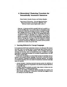
IV. RESULTS AND DISCUSSION Note that the purpose of this paper is not to develop a hypothesis for sound localization but to propose new methods for the analysis of spatio–temporal multidimensional time series. A. MEG Spatio–Temporal Patterns First, we confirmed there was no observation of a MEG response produced by the individual click trains of width and interval nor by the monoaural cue with offset [see Fig. 1(a) for – ]. Fig. 2 shows a typical MEG time series displayed by (a) time course stacks for all of the detectors and by (b) iso-contour maps (iso-contour line: 100 fT, black lines: positive, gray lines: negative). In each of Fig. 2(a) and (b), types onset (S C), offset (C S), left-shift (C LL), and right-shift (C RL) are placed at the top left, top right, bottom left, and bottom right, respectively. Each iso-contour map shows, in the azimuthal equidistant chart manner (top view, nose: left), the MEG spatial pattern around the peak latency, which is indicated by the triangular mark in the corresponding time course stack. Note that the spike-like waves around 0 ms, as shown in Fig. 2(a), are artifacts caused by the triggers for averaging. From typical spatio–temporal auditory MEG time series [33], the following two points may be noted. i) In the temporal activities, the significant activities are seen approximately from 60 to 300 ms for all of the types, despite slight differences.

Fig. 2. Typical MEG time series. (a) Time course stacks for all of the detectors. (b) Iso-contour maps at the time sample points indicated by the triangular marks in (a) (top view, iso-contour line: 100 fT, black lines: positive, gray lines: negative). The change of the states is written on the left-hand side of each illustration.

ii) In the spatial patterns, the significant patterns are seen in and around auditory cortexes located in both temporal areas. We found similar time course stacks and iso-contour maps for the 26 other experiments. We could not thereby discover the inherent characteristics among the MEG time series to evaluate similarity of them even qualitatively by only observation of the time course stacks and iso-contour maps. Needless to say, the quantitative evaluation of similarity among the MEG time series by such observation is almost impossible. B. Hierarchical Clustering Performance For all 30 MEG time series, the waveforms for durations of in (5) 60–300 ms were extracted and the partition number was set to 10 (out of a maximum 64), such that the cumulative contributions exceeded 97% for all. Fig. 3(a) shows the hierarchical clustering result of Method I by dendrogram (hierarchical cluster tree). The numbers along the horizontal axis of the dendrogram indicate the experiment numbers listed in Table I. The vertical axis indicates the distance between


Fig. 3. Results of Method I. (a) Dendrogram (horizontal axis: experiment number, vertical axis: distance). (b)–(e) Breakdown clusters in case of division by four (circle: type onset, cross: type offset, left arrow: type left-shift, right arrow: type right-shift).

357

Fig. 4. Results of Method II. Explanations of (a)–(e) are the same as in Fig. 3(a)–(e).

i) one MEG time series and another MEG time series; ii) an MEG time series and a cluster; iii) two clusters. The dendrogram is useful for validating the clustering result, independently of the brain researcher’s subjective interpretations. If the within-cluster distances are small and also the inter-cluster distances are large, then the clustering result is valid. Observing Fig. 3(a) from this validity standpoint, the MEG time series may be clustered into four groups. Fig. 3(b)–(e) show the four breakdown clusters. The circles, crosses, left arrows, and right arrows indicate types onset, offset, left-shift, and right-shift, respectively. In the same manner, the clustering results of Methods II and III are also shown in Figs. 4 and 5, respectively. For comparison purposes, four groups are also used for the breakdown clusters of Methods II and III, as shown in Figs. 4(b)–(e) and 5(b)–(e), respectively. From the validity standpoint, the clustering results of Methods II and III are evaluated as follows. For Method II, one can see two large obvious clusters in Fig. 4(a). The first two clusters [Fig. 4(b) and (c)] and the last two [Fig. 4(d) and (e)] should be separately merged. On the contrary, for Method III, there is no obvious division of the cluster in Fig. 5(a). The breakdown clusters are almost meaningless. Regarding Methods IV and V, only dendrograms are shown in Fig. 6 because the within-cluster distances are too large that the breakdown representation is definitely meaningless. The same was found when employing the largest eigenvalue of the difference (see Section I) as a distance measure. Note that the distances scaled by the vertical axes of the dendrograms in Figs. 3–6 have relative meaning only within each figure but do not have absolute meaning when comparing figures.

Fig. 5. Results of Method III. Explanations of (a)–(e) are the same as in Fig. 3(a)–(e).

Apart from the somewhat qualitative validation, the cophenetic correlation coefficient was then used for the quantitative one. The cophenetic correlation coefficient is a correlation coefficient of pairwise distances between before-and-after hierarchical clustering to validate the distortion by the clustering procedure. The closer to one the cophenetic correlation coefficient is, the smaller the distortion. The cophenetic correlation coefficients of Methods I to V were 0.70, 0.58, 0.53, 0.76, and 0.72,

358

Fig. 6. Dendrograms of (a) Method IV. (b) Method V. Explanation is the same as in Fig. 3(a).

respectively. The reason Methods IV and V have relatively high correlation values is that those two have no obvious breakdown clusters and, hence, just maintain the original distribution of the MEG time series. On the other hand, the correlation value of Method I, 0.7, can be considered high despite having obvious breakdown clusters. Those validation results indicate the following three points. i) The proposed distance is more appropriate than the Euclidian distance for evaluating the dissimilarity in terms of the nature of the MEG recording. ii) The half-inverse transform is necessary for scaling normalization. iii) The grouping algorithm based on the Ward method is more appropriate than the single and complete linkages. Let us discuss the clustering results of Methods I to III from the standpoint of brain function. Methods IV and V are excluded because their clustering results are invalid. We named the types of stimuli by expected perceptions produced by the stimuli. In fact, healthy subjects can separately perceive types onset, offset, left-shift, and right-shift, and thereby, the perception can be clustered by the types of stimuli as expected. Being independent of the perceptions, the stimuli, as stereo time series of ITD, can be also clustered by the names of types using their crosscorrelation functions between the left and right time series. The perception occurs at the end of the sequence through which each stimulus has been represented by its spatio–temporal brain activity. The spatio–temporal brain activity is partially recorded using MEG, where it is also independent of the sequence. Under such


circumstances, in the breakdown clustering results of Method I [Fig. 3(b)–(e)], types onset and offset are completely clustered separately. Types left-shift and right-shift are almost completely divided with only a couple of exceptions. On the other hand, no obvious characteristic is found in the results of Method II [Fig. 4(b)–(e)], and nothing, except that type offset is solely clustered, is found in the results of Method III [Fig. 5(b)–(e)]. It is important that the results of Method I, which is based on the independent MEG recording, namely, on unsupervised learning, are significantly consistent with the clustering of the stimuli and perceptions. However, encountered difficulties are as follows to answer the question what the explicit characteristics in the MEG time series are related to the results of Method I. Previous brain studies for sound localization sought to discover laterality [32] and contralaterality [34] in the latency and magnitude of brain activity using MEG, EEG, and/or functional magnetic resonance imaging (fMRI). Since the proposed distance , , and the (16) depends only on the orthogonal matrices partition number , the latency of the brain activity does not affect the clustering results (but affects the filtering results). If laterality or contralaterality exists in any magnitude, then a clustering result such as that of Method I may be obtained. However, laterality or contralaterality is difficult to discover by only observation of the iso-contour maps, as shown in the bottom row of Fig. 2(b), because the spatial activation patterns can be seen in and around both auditory cortexes regarding types left-shift and right-shift. Thus, it is difficult to reduce the results of Method I to known brain characteristics or the spatio–temporal MEG time series. On the other hand, to discuss new brain characteristics is not the main subject of this paper. We have an implicit answer to the question that the results of Method I are caused by , , and inherited from the the extracted information as difference of the covariance structure of the MEG time series. In the practical application of the proposed hierarchical clustering, there remains an inconvenience. The proposed distance (16) is sensitive to MEG and/or EEG spatial patterns. The relative location between the brain and the MEG and/or EEG detectors must therefore be fixed throughout the experiments. To support the hypothesis-free standpoint, the number of experiments becomes large. The necessary time for the experiments increases accordingly. To avoid or to reduce not only prediction and habituation but also fatigue of the subject, it is important to obtain reliable MEG and/or EEG time series. There are limitations in the psychophysical techniques for overcoming the problem. If the hierarchical clustering is performed for the MEG and/or the EEG time series is recorded at different locations, a method for adjusting the locations will be required. C. Filtering Performance We first selected the MEG time series corresponding to LS C, LL C, RS C, and RL C, and then set C LS for the target of the filtering (25). The duration of MEG time series and and the partition number in (5) to determine in (25) were the same values used in the hierarchical clustering (see Section IV-B). Fig. 7 shows the filtering results. The solid, dashed, dotted, and alternately long and short dashed lines inC, RS C, LL C, dicate the filtering results from RL and LS C, respectively. Being different from the hierarchical


359

between data to be analyzed and the origin of the data. We hope that these methods will help the analysis of spatio–temporal multidimensional time series. As an example, we applied the proposed methods to the analysis of MEG and/or EEG time series. The results indicated the effectiveness of those methods. Since the proposed methods do not require any a priori information, it will support studies by brain researchers from the hypothesis-free standpoint. In MEG and/or EEG analysis, inverse methods for estimating the location of current dipoles as the sources of MEG and/or EEG have been the mainstream to date. However, the proposed methods are categorized as noninverse methods. We also hope that in the analysis of MEG and/or EEG time series, the proposed methods will be beneficial as noninverse methods. APPENDIX A

! !

!

!

!

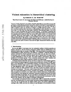
Fig. 7. Filtering results. The target is C LS. Those lines are the temporal contributions of the target (solid: RL C, dashed: RS C, dotted: LL C, alternately long and short dashed: LS C).

clustering results, one can see that the filtering results clarify the temporal information of the similarity between the MEG time series. The MEG time series that have the same shift direction as the target’s are similar to the target for durations of 100–150 ms. However, this situation is not always true for durations of 200–250 ms. Although there is room for argument regarding this situation from the standpoint of the brain function, unfortunately, we have not found previous studies appropriate for evaluation. The argument would therefore lead us into develop our hypothesis of the spatio–temporal structure in sound localization, and that is not the main subject of this paper. The important point is that the filtering can produce useful information for analyzing brain functions and for developing hypotheses of these.

Proof: Symmetry Property (18): From (15)

such that with (16) (34) is an orthogonal matrix, and hence, each column or Here, row is normalized. Therefore

(35) From (16), (34), and (35)

V. CONCLUSION We proposed hierarchical clustering and filtering methods for the analysis of spatio–temporal multidimensional time series, both of which employed a new pseudo distance. This pseudo distance is calculated using only two subspaces that are orthogonal complements with respect to each other and a partition number determined by eigenvalue decomposition of the variance–covariance matrix of the spatio–temporal multidimensional time series. The calculation process of not only this pseudo distance but also other previously proposed distances loses a large amount of information from the original spatio–temporal multidimensional time series. When a distance is determined, there exists a tradeoff relationship between sensitivity and robustness. The desired distance is sensitive to the features of interest and insensitive to the others. If one is interested in spatial patterns, this pseudo distance may be appropriate. In clustering, the grouping algorithm is also important. The Ward method, known with the Euclidean distance, is modified to fit the pseudo distance. Of the lost information, by the pseudo distance measure, the filtering can recover part of the temporal information. We also proposed a normalization method when there is a mathematical transform

Proof: Triangle Inequality Property (19): First, and are determined as follows: trices

ma-

diag

(36)

diag

(37)

Using (36) and (37), for example, the following notations regarding (15) will be possible:

360


Assuming

Finally, (23) is proved. Note that the following techniques are used in the above deformation. i) In (39) to (40), the underlined section of (39) is cyclically multiplied to the first product of the term. ii) In (40) to (41), the eigenvalue decomposition is performed for the underlined section of (40). iii) The underlined section of (41) is the identity matrix. iv) Equation (42) is the Frobenius norm by trace notation.

with (15)

ACKNOWLEDGMENT The authors would like to thank Dr. N. Fujimaki of Communications Research Laboratory, Kobe, Japan, for his helpful suggestions. REFERENCES

APPENDIX B Proof: Equivalent Property (23): With (22) and (36), let be

(38) The right-hand side term of (23) is denoted by . Using (38), we obtain

tr tr tr (39) tr (40) tr (41) tr

(42)

(43)

[1] M. R. Anderberg, Clustering Analysis for Application. New York: Academic, 1973. [2] J. H. Ward, “Hierarchical grouping to optimize an objective function,” J. Amer. Statist. Assoc., vol. 58, pp. 236–244, 1963. [3] D. Wishart, “An algorithm for hierarchical classifications,” Biometrics, vol. 25, pp. 165–170, 1969. [4] J. B. Macqueen, “Some methods of classification and analysis of multivariate observations,” in Proc. 5th Berkeley Symp. Math. Stat. Prob., 1967, pp. 281–297. [5] A. Gersho, “On the structure of vector quantizers,” IEEE Trans. Inform. Theory, vol. IT-28, pp. 157–166, 1982. [6] Y. Linde, A. Buzo, and R. M. Gray, “An algorithm for vector quantizer design,” IEEE Trans. Commun., vol. COM–28, pp. 84–95, 1980. [7] S. P. Lloyd, “Least squares quantization in PCM,” IEEE Trans. Inform. Theory, vol. IT–28, pp. 129–137, 1982. [8] W. H. Equitz, “A new vector quantization clustering algorithm,” IEEE Trans. Acoust., Speech. Signal Processing, vol. 37, pp. 1568–1575, Oct. 1989. [9] R. L. Bottemiller, “Comments on a new vector quantization clustering algorithm,” IEEE Trans. Signal Processing, vol. 40, pp. 455–456, Feb. 1992. [10] P. Wahlberg and G. Lantz, “Methods for robust clustering of epileptic EEG spikes,” IEEE Trans. Biomed. Eng., vol. 47, pp. 857–868, 2000. [11] A. B. Geve and D. H. Kerem, “Forecasting generalized epileptic seizures from the EEG signal by wavelet analysis and dynamic unsupervised fuzzy clustering,” IEEE Trans. Biomed. Eng., vol. 45, pp. 1205–1216, Oct. 1998. [12] G. Zouridakis, N. N. Bourtros, and B. H. Jansen, “A fuzzy clustering approach to study the auditory P50 component in schizophrenia,” Psych. Res., vol. 69, pp. 169–181, 1997. [13] G. Zouridakis, B. H. Jansen, and N. N. Boutros, “A fuzzy clustering approach to EP estimation,” IEEE Trans. Biomed. Eng., vol. 44, pp. 673–679, Aug. 1997. [14] R. O. Schmidt, “Multiple emitter location and signal parameter estimation,” IEEE Trans. Antennas Propagat., vol. AP-34, pp. 276–280, 1986. [15] J. C. Mosher, P. S. Lewis, and M. Leahy, “Multiple dipole modeling and localization from spatio–temporal MEG data,” IEEE Trans. Biomed. Eng., vol. 39, pp. 541–557, June 1992. [16] K. Sekihara, D. Poeppel, A. Marantz, H. Koizumi, and Y. Miyashita, “Noise covariance incorporated MEG-MUSIC algorithm: A method for multiple-dipole estimation tolerant of the influence of background brain activity,” IEEE Trans. Biomed. Eng., vol. 44, pp. 839–847, Sept. 1997. [17] E. Oja, Subspace Methods of Pattern Recognition. London, U.K.: Research Studies, 1983. [18] S. U. Pillai, Array Signal Processing. New York: Springer-Verlag, 1989. [19] C. D. Tesche, M. A. Uusitalo, R. J. Ilmoniemi, M. Huotilainen, M. Kajola, and O. Salonen, “Signal-space projections of MEG data characterize both distributed and well-localized neuronal sources,” Electroenceph. Clin. Neurophysiol., vol. 95, pp. 189–200, 1995. [20] W. Menke, Geophysical Data Analysis: Discrete Inverse Theory. New York: Academic, 1989. [21] M. Hämäläinen, R. Hari, R. J. Ilmoniemi, J. Kuutila, and O. V. Lounasmaa, “Magnetoencephalography—Theory, instrumentation, and applications to noninvasive studies of the working human brain,” Rev. Modern Phys., vol. 65, pp. 413–497, 1993.


[22] J. C. Mosher, R. M. Leasy, and P. S. Lewis, “EEG and MEG: Forward solutions for inverse methods,” IEEE Trans. Biomed. Eng., vol. 46, pp. 245–259, Mar. 1999. [23] D. B. Geselowithz, “On the magnetic field generated outside an inhomogeneous volume conductor by internal current sources,” IEEE Trans. Magn., vol. MAG-6, pp. 346–347, 1970. [24] J. Sarvas, “Basic mathematical and electromagnetic concepts of the biomagnetic inverse problem,” Phys. Med. Biol., vol. 32, pp. 11–22, 1987. [25] R. C. Barr, T. C. Pilkington, J. P. Boineau, and M. S. Spach, “Determining surface potentials from current dipoles, with application to electrocardiography,” IEEE Trans. Biomed. Eng., vol. BME-13, pp. 88–92, 1966. [26] D. Yao, “Electric potential produced by a dipole in a homogeneous conducting sphere,” IEEE Trans. Biomed. Eng., vol. 47, pp. 964–966, July 2000. [27] A. W. Mills, “Lateralization of high-frequency tones,” J. Acoust. Soc. Amer., vol. 32, pp. 132–134, 1960. [28] E. A. G. Shaw, “Transformation of sound pressure level from the free field to the eardrum in the horizontal plane,” J. Acoust. Soc. Amer., vol. 56, pp. 1848–1861, 1974. [29] W. A. Yost, “Discriminations of interaural phase difference,” J. Acoust. Soc. Amer., vol. 55, pp. 1299–1303, 1974. [30] J. O. Nordmark, “Biaural time discrimination,” J. Acoust. Soc. Amer., vol. 60, pp. 870–880, 1976. [31] D. W. Grantham and F. L. Wightman, “Delectability of varying interaural temporal difference,” J. Acoust. Soc. Amer., vol. 63, pp. 511–523, 1978. [32] P. Ungan, B. S¸ahino˘olu, and R. Utkuçal, “Human laterality reversal auditory evoked potentials: Stimulation by reversing the interaural delay of dechotically, presented continuous click trains,” Electroenceph. Clin. Neurophysiol., vol. 73, pp. 306–321, 1989. [33] N. Nakasato, S. Fujita, K. Seki, T. Kawamura, A. Matani, I. Tamura, S. Fujiwara, and T. Yoshimoto, “Functional localization of bilateral auditory cortices using an MRI-linked whole head magnetoencephalography (MEG) system,” Electroenceph. Clin. Neurophysiol., vol. 94, pp. 183–190, 1995. [34] M. G. Woldorff, C. Tempelmann, J. Fel, C. Tegeler, B. GaschlerMarkefski, H. Hinrichs, H. J. Heinze, and H. Scheich, “Lateralized auditory spatial perception and the contralaterality of cortical processing as studied with functional magnetic resonance imaging and magnetoencephalography,” Human Brain Mapping, vol. 7, pp. 49–66, 1999.

Ayumu Matani (M’96) received the B.S., M.S., and Ph.D. degrees from Osaka University, Osaka, Japan, in 1989, 1991, and 1998, respectively. He was with Osaka Gas Co. Ltd., Japan, from 1991 to 1995 and with Nara Institute of Science and Technology, Nara, Japan, from 1995 to 1998. He is now an Associate Professor with the Graduate School of Frontier Sciences, the University of Tokyo, Tokyo, Japan. His research interests include signal processing for complex biological systems.

361

Yasushi Masuda (M’02) received the B.S. degree from Osaka University, Osaka, Japan, in 1996 and the M.S. and Ph.D. degrees from Nara Institute of Science and Technology, Nara, Japan, in 1998 and 2002, respectively. He is now a Research Associate with the Department of Gerontechnology, National Institute for Longevity Sciences, Aichi, Japan. His research interests include human brain function and its measurement.

Hideaki Okubo received the B.S. and M.S. degrees from the University of Tokyo, Tokyo, Japan, in 1999 and 2001, respectively. He is now with Core Technology and Network Company, SONY Corporation, Tokyo. His research interests include biaural auditory response and its MEG analysis.

Kunihiro Chihara (M’77) received the B.S., M.S., and Ph.D. degrees from Osaka University, Osaka, Japan, in 1968, 1970, and 1973, respectively. He was with Osaka University from 1973 to 1992. He is now a Professor with the Graduate School of Information Science, Nara Institute of Science and Technology, Nara, Japan. His research interests include biomedical signal processing, acoustical instrumentation, three-dimensional visualization, virtual reality, digital archiver, and multimedia.