Using Hierarchical Clustering for Learning the Ontologies used in Recommendation Systems Vincent Schickel-Zuber
Boi Faltings
Swiss Federal Institute of Technology - EPFL Artificial Intelligence Laboratory Lausanne, Switzerland
Swiss Federal Institute of Technology - EPFL Artificial Intelligence Laboratory Lausanne, Switzerland
[email protected]
[email protected]
ABSTRACT Ontologies are being successfully used to overcome semantic heterogeneity, and are becoming fundamental elements of the Semantic Web. Recently, it has also been shown that ontologies can be used to build more accurate and more personalized recommendation systems by inferencing missing user’s preferences. However, these systems assume the existence of ontologies, without considering their construction. With product catalogs changing continuously, new techniques are required in order to build these ontologies in real time, and autonomously from any expert intervention. This paper focuses on this problem and show that it is possible to learn ontologies autonomously by using clustering algorithms. Results on the MovieLens and Jester data sets show that recommender system with learnt ontologies significantly outperform the classical recommendation approach.
Categories and Subject Descriptors
Unfortunately, collaborative filtering suffers from scalability[10] and cold-start problems[11]. The former problem is due to the neighborhood of items that must be constructed in order to extract the experience of similar users, while the latter is a consequence of the unconstrained search space that requires many items to be rated in order to find the right neighbors. To constrain the search space, a novel technique called ontology filtering has been proposed([12], OF). This approach infers preference ratings of items based on the ratings of known items, and their relative position in an ontology. The ontology is defined as a multi-inheritance graph structure, where an edge represents one or more features, and an item is an instance of at least one concept. Given this ontology, OF associates with each concept c an a-priori score, APS(c), which captured the information contained by a concept. To predict the user’s rating of an unrated concept y, the system uses knowledge of the normalized rating S(x) of the closest concept x, and the lowest common ancestor to concepts x and y in the ontology. Formally, the inference is as follows:
H.1.2 [Information Systems]: User/Machine systems
General Terms Algorithms, Experimentation, Performance.
Keywords Ontology, Recommendation System, Clustering.
1.
INTRODUCTION
With the growing importance of the internet, people are becoming overwhelmed by information. Recommender systems have been designed to help people in this situation by finding the most relevant items based on the preferences of the person and others. Today, the most widely used technique is item-based collaborative filtering, ([10], CF). Given a user, the goal of CF is to recommend items based on the experience of the user as well as other similar users. Collaborative filtering captures the user’s experience by asking him to rate the items he has interacted with, and stores all these historical data in a user-item matrix R.
Permission to make digital or hard copies of all or part of this work for personal or classroom use is granted without fee provided that copies are not made or distributed for profit or commercial advantage and that copies bear this notice and the full citation on the first page. To copy otherwise, to republish, to post on servers or to redistribute to lists, requires prior specific permission and/or a fee. KDD’07, August 12–15, 2007, San Jose, California, USA. Copyright 2007 ACM 978-1-59593-609-7/07/0008 ...$5.00.
µ S(y|x) =
AP S(lca) AP S(x)
¶ S(x) + (AP S(y) − AP S(lca))
(1)
where lca is the lowest common ancestor between concepts x and y. Informally, Equation 1 infers the score of concept y by first looking at the closest concept x that has a score. Then, it looks at the commonalities between the concept x and lca, which measures how much information is preserved going up the tree. Finally, we add the information gained by adding the extra features between concepts lca and y. Thus, the recommended items are the ones achieving the best score. Note that contrary to CF, OF only uses the user’s preferences for the inference process. To illustrate these two approaches, we are going to build a simple recommendation system for helping a user choose a means of transportation. Figure 1(a) shows the matrix R that contains the preferences of three users: David, Paolo, and Alex. Such a matrix is the input of traditional recommendation system. The ratings range from 1 to 5, and the symbol x means that no preferences were stated by the users. Let’s now imagine that Alex is planning to visit one of his friends who lives far away. Further imagine that to get there, Alex can only use a car or the train. Bike David 4 Paolo x Alex 4
Car 5 x x
Train x 5 x
(a) user-item matrix R
Plane x 4 4
Bike Car Train Plane
Bike Car Train Plane 1 -1 x 0 -1 1 x x x x 1 -1 0 x -1 1 (b) item-item matrix S
Figure 1: (a) matrix R, while (b) is matrix S computed from (a) To use item-based collaborative filtering, the system starts by constructing the item-item similarity matrix S (Figure 1(b)). This
matrix is constructed from R using Equation 3 (see section 2.1), where Si,j is the similarity between items i and j. Given Alex, the predicted rating of an item i is computed using a weighted average of Alex’s ratings by the similarity of closest neighbors to i. ˆ Alex,i , is computed as Formally, the predicted rating of item i, R follows[8]: P ˆ Alex,i = Ri + R
j∈ K (Si,j
P
∗ (RAlex,j − Rj ))
j∈ K
(2)
|Si,j |
where K is the set of the k-closest neighbors to item i. If we set |K| to 2, the predicted ratings of items train and car become 5 ˆ Alex,train = R ˆ Alex,car = 5). As both items have identical (i.e.: R predicted ratings, CF would recommend both to Alex.
tologies, and that ontology filtering with these learnt ontologies still outperforms item-based collaborative filtering. We also define a new algorithm that is capable of building multi-hierarchical ontologies, and show that this more complex structure brings some robustness to the prediction accuracy. Finally, we provide fresh experimental results concerning the behavior of hierarchical clustering algorithms and ontology filtering recommendation system on two data sets that contain real users data (MovieLens and Jester). The rest of this paper is organized as follows. First, we introduce all the necessary background that is used throughout the paper, while our algorithms used to learn and select which ontology to use are presented in Section 3. In the experiment section, we give detailed results of the behavior of learnt ontologies and show that these learnt ontologies actually outperform item-based collaborative filtering on the Jester and MovieLens data sets. Finally, we conclude this paper in Section 5.
km 00 >1
On-wheels
Train
Individual
Private
nd la nO
In -a ir
S(Car|Bike), the recommended item will be the train, . Given Alex’s preferences, it is quite easy to see that the prediction made by ontology filtering is more coherent than the one from CF; as the majority of users who like to travel by public transport would also prefer to travel by train rather than by car. This behavior is represented by the fact that both concepts Plane and Train share the same ancestor, which is different from the ancestor of the concept Car. Moreover, if Alex liked to travel by car, then he would have stated it; as users tend to state the preferences they really care about. Note also that ontology filtering uses less data than collaborative filtering as the structure of the ontology limits the search space to the closest concept with a rating. In E-commerce applications, many items with new features are being constantly added to E-catalogs. Inversely, old items are removed from the E-catalogs as they become obsolete. In such situations, it is unrealistic to imagine that such an ontology can be maintained by a group of experts. Furthermore, the ontology does not exploit the similarities as expressed by the matrix S. Finally, we think that using the same ontology for every user is suboptimal as each user perceives reality differently from others. This paper focuses on the problem of learning these ontologies using unsupervised learning algorithms. Given this set of ontologies and a particular user, we propose another algorithm to select which ontology to use based on the user’s preferences. We show that hierarchical clustering algorithms can be used to learn the on-
2.
BACKGROUND
In both collaborative filtering and ontology filtering, users state their preferences by rating a set of items, which are then stored in the user-item matrix R. Formally, this matrix contains all the users’ profiles, where the rows represent the users U = {u1 , , um }, the columns correspond to the set of items I = {i1 , , in }, and Ru,i is the rating assigned to item i by the user u. It is common practice to denote the average rating of user u by R¯u , and the average rating of the item i by R¯i .
2.1
Collaborative Filtering
Item-based collaborative filtering works by finding similar items to the ones bought by the user, and then combines those similar items into a recommendation list. The fundamental assumption behind CF is that similar users like similar items. Formally, the recommendation process is as follows. First, CF computes the pairwise similarities between all the items in the matrix R. These similarities are computed using the adjusted cosine similarity metric, which is defined as follows[10]: P
sim(i, j) = qP
− R¯u )(Ru,j − R¯u ) q ¯ 2 P ¯ 2 u∈ U (Ru,i − Ru ) u∈ U (Ru,j − Ru ) u∈ U (Ru,i
(3)
Once the item-item similarity matrix S has been computed, the predicted rating of an item i is computed using the k most similar items to i, which is commonly known as i’s neighborhood. Thus, the predicted rating is computed using a weighted average of the user’s ratings by the similarity of item i’s neighborhood (Equation 2). Once all the possible items to be recommended have been rated, we simply select the N items with the best predicted rating. This selection process is called the top-N recommendation strategy. By working on the items rather than on the users, CF is able to reduce the search space, which makes it scalable to E-commerce environments. For example, Amazon.com with its 29 million customers uses item-based collaborative filtering to personalize its recommendations([7]). However, with thousands of items in current E-commerce catalogs, the search space remains huge and unconstrained. Thus, CF requires the user to rate many items in order to find highly correlated neighbors. Moreover, the recommendation accuracy is greatly influenced by the size of the item’s neighborhood.
2.2
Ontology Filtering
In ontology filtering, two input structures are required: the users’ historical data R and an ontology modeling the domain. The on-
tology is defined as a directed acyclic graph, where an edge is a binary isa relation that models some features. Note that the features are usually not made explicit when defining the ontology. Take for example a bottle of red and a bottle of white wine. Both bottles would be children of the wine concept, and the color of the wine would be the feature that differentiates the red wine sub-concept from the white wine one. However, the taste would also be a feature that differentiates these two subconcepts, but this feature will remain implicit. Ontology filtering starts by extracting the information contained in the ontology. This is achieved by computing an expected normalized score of each concept c, known as the a-priori score, AP S(c). The APS is defined as a lower bound of the actual score an instance of the concept might have. We define the APS of a concept c as: AP S(c) =
1 nc + 2
(4)
where nc is the number of descendants of the concept c [12]. As for collaborative filtering, the user expresses his preferences by rating a set of items. For each rated item, the algorithm extracts its features and computes the score of each concept based on the specified rating. Unfortunately, it is very unlikely that the user was able to give enough ratings to compute the score of all the concepts in the ontology. To overcome this problem, for all the concepts y without any score, OF will infer it by transferring the score of the closest concept x (Equation 1). In Equation 1, the coefficient α(x, lca) = AP S(lca)/AP S(x) represents the ratio of features which are both liked in the concept x and lca, while β(y, lca) = AP S(y) − AP S(lca) measures how much the new features added to the lowest common ancestor will be liked[12]. The former coefficient represents the score being preserved when traveling upwards to the concept lca, while the latter contains the score gained by traveling downwards from the lca . Note that the inference assumes that the relationships between real scores are the same as those between a-priori scores. To minimize the error during the inference, OF needs to find the closest concept x to any given concept y in the ontology. To perform this crucial task, Schickel and Faltings[12] derived a new distance function from Equation 1 called OSS. In [13], OSS was refined and it was showed that it actually outperforms state of the art metrics on WordNet and the GeneOntology. Formally, OSS defines the distance between concepts x and y in an ontology as follows: D(x, y) =
log(1 + 2β(x, lca)) − log(α(y, lca)) maxD
(5)
where α and β are the same coefficients as in Equation 1.
2.3
CF vs. OF
There are three fundamental differences between ontology filtering and collaborative filtering. First, rather than using the item-item similarity matrix S, the item similarity in ontology filtering is restricted to a hierarchical ontology. This reasoning topology allows to constrain the search space, which limits the number of ratings the system has to elicit from the user. Experimental results have shown that ontology filtering leads to significant improvements in the prediction accuracy over CF, especially when little data about the user is known [12]. Second, ontology filtering infers the missing score from the closest concept with preferences rather than from a neighborhood. As less data is required, it makes this approach much more scalable than collaborative filtering. Finally, missing user preferences are inferred from the user’s past experience instead of using other people’s preferences, which increases the personalization of the recommendations list[12]. The main assumption in ontology filtering is that an ontology
modeling the items’ features exists. Unfortunately, this is an unreasonable assumption when we consider the fact that hundreds of items get added or removed from E-catalogs each day. Furthermore, the ontology should capture the item similarities as expressed by the user population. Thus, new techniques are required for building these ontologies automatically, and without any user intervention. Moreover, collaborative filtering proved that using collaborative data increased the prediction accuracy. Thus, we show that it is possible to construct these ontologies from the matrix R using clustering algorithms, which allows the ontologies to capture the knowledge of a user population.
3.
LEARNING THE ONTOLOGIES
Users are being continuously solicited to express ratings on items they have either seen or bought. As a consequence, rated items are becoming widely available. For example, buyers on eBay.com are invited to evaluate a seller each time they have bought an item, while on YouTube.com, users can rate videos they have seen. Microsoft Office also invites users to rate the help tips they have received. Given these ratings, our first contribution is to show that hierarchical clustering algorithms can successfully be used to learn a set of hierarchical trees that will later be used as ontology in the ontology filtering approach.
3.1
Clustering Algorithms
Over the years, researchers in the data mining community have proposed many clustering algorithms in order to perform unsupervised learning. These algorithms can be classified into at least six categories[6]: fuzzy clustering, nearest-neighbor clustering, hierarchical clustering, artificial neural networks for clustering, statistical clustering algorithms, and density-based clustering. In this paper, we are interested in building hierarchical ontologies. Thus, we will focus our research on hierarchical clustering algorithms, which can build such a structure. Hierarchical algorithms can in fact be categorized into two subcategories: distance-based clustering and conceptual-based clustering. Both approaches construct hierarchical trees, but they use very different data representation. With distance-based clustering, objects are represented in a well defined space, like a vector in a 2D cartesian space. Thus, two or more objects will be assigned to the same cluster if they are close according to a given distance function. However, with concept-based clustering, objects are defined by a set of concepts, where a concept is usually an attribute-value pair. Given this representation, two or more objects belong to the same cluster if they share common concepts.
3.1.1
Distance-Based Clustering
When considering distance-based clustering, there are in fact two distinct ways to build a hierarchical tree: the bottom-up or topdown approach. These approaches are respectively known as the agglomerative clustering and partitional clustering. Partitional algorithms start by assigning all the items to be clustered into a unique cluster. Then, one cluster Cj is chosen and is then further bisected into Ci , where i ∈ [1, 2] clusters. For each item in Cj , we assign them to the cluster Ci that optimizes a distance function. This process continues until either all the items are found on the leaf of the tree, or the number of clusters has met a given threshold θ. Inversely, agglomerative clusterings assign each item to its own cluster Ci ,where i ∈ [1, n]. Then, the two closest clusters are merged into a unique cluster. As for partitional clustering, the process reiterates until the entire tree is created, or the number of clusters has met a given threshold θ.
The main advantage of partitional algorithms is their low complexities, which allow them to cluster millions of elements. However, partitional algorithms can suffer from local minima, and are dependent on the input order of the items. On the other hand, in general, agglomerative algorithms give better clustering solutions than partitional algorithms. However in [15], Zhao et Karypis have shown that for clustering document data sets, partitional clusterings always led to better clustering solutions than agglomerative ones. The main disadvantage of agglomerative clusterings is their complexities. In the first step of the algorithm, all pairwise similarities must be computed, leading to a complexity of O(n2 ).
3.1.2
Concept-Based Clustering
The most famous (incremental) conceptual clustering algorithm is COBWEB, which was introduced by Fisher[3] in 1987. Contrary to the first two clustering algorithms, items need to be represented by a set of attribute-value pairs. For example, a mammal could be modeled by the attributes body cover, heart chamber and body temperature, which have the following respective values: hair, four, and regulated. Given this representation, a node (class) in the tree represents the probability of the occurrence of each attribute-value pair for all the instances of that node. Thus, the root node represents all the possible attribute-value pairs defined in the system, and nodes become more specific as we go down the tree. For each item to classify, COBWEB will incrementally incorporate it to the classification tree by descending the tree along an appropriate path, updating counts along the way, and performing one of the four operators at each level. These operators are as follows. • add - adds the item to an existing class, • create - creates a new class for the item, • merge - merges two classes, and • split - splits a class into several ones. As item are added incrementally, the ordering of the initial input can lead to different classification results. To reduce this problem, [3] uses the operators merge and split. Furthermore, node merging and splitting are roughly inverse operators, and allow COBWEB to move bidirectionally through a space of possible hierarchies. The choice of the operator will by be guided by a category utility function that rewards traditional virtues held in clustering, i.e.: similar objects should appear in the same class, while dissimilar ones should be in different classes. Thus, the category utility function is in fact a trade off between intra-class similarity and inter-class dissimilarity of items. A detailed explanation of category utility can be found in [3]. One of the main advantages of COBWEB over the partitional and agglomerative clustering algorithms is that it allows new items to be added incrementally to the classification tree, without recomputing the entire tree. Note also that the process is bidirectional, which means that a node that has been created can be merged again later on. Second, conceptual clustering uses probabilistic descriptions of concepts, rather than distances. Furthermore, the operators merge and split guarantee homogeneity of the content of the class. However, COBWEB has some known problems. First, the classification tree is not height-balanced which leads to space and time complexity to degrade dramatically. The overall complexity of COBWEB is exponential to the number of attributes, as the category utility function requires analyzing all the attribute-value pairs. Despite these problems, and because most authors assume that the number of attributes is small, COBWEB is becoming increasingly popular in the Semantic Web. For example in [1], Clerkin et al. proposed to use COBWEB directly on the user-item matrix R to build meaningful hierarchical ontologies of songs. To do this, they
consider each item as an attribute, and the rating assigned to each item is transformed in the feature value good if it had a rating superior or equal to 4, or bad otherwise. In [14], Sea and Ozden have used COBWEB to generate the ontology from files’ description in order to perform ontology-based file naming.
3.2
Learning Hierarchical Ontologies
In the collaborative filtering research community, it is an established fact that users can be categorized in different communities, and that a community of users behaves in a similar fashion. Following these observations, we believe that using just one ontology for all the users is not appropriate, and that it is better to select which ontology to use based on the user’s preferences. Following this, we will use many clustering algorithms to generate a whole set of ontologies Λ, and then select the best ontology based on the user’s preferences. In order to generate these ontologies, we will use different distance functions or criteria functions ([15]). Table 1 shows the criteria functions that we use in our algorithms, where k is the number of clusters to consider, nr denotes the number of elements in cluster r, Cr is the rth cluster, Crt is the centroid of the rth cluster, and sim(i, j) is the similarity between items i and j. Table 1: Criteria functions used for distance-based clustering ³P ´ P 1 I1 maximize kr=1 n1r sim(i, j) i,j∈Cr P P 2 I2 maximize kr=1 i∈Cr sim(i, Crt ) Pk 3 E1 minimize r=1 nr sim(Crt , C) P r 4 G1 minimize kr=1 Pcut(Cr ,C−C sim(i,j) 5 6 7 8 9
H1 H2 slink clink U P GM A
i,j∈Cr
maximize IE11 maximize IE12 maxi∈Ci ,j∈Cj sim(i, j) mini∈Ci ,j∈Cj sim(i, P j) maximise ni1,nj i∈Ci ,j∈Cj sim(i, j)
During partitional clustering, a distance function is required in order to assign each item in Cj to the cluster Ci that optimizes the distance function. Thus, our algorithm will use the criteria I1 , I2 , E1 , H1 , and H2 as distance functions. I1 and I2 are internal criteria functions that focus on producing a clustering solution that optimizes the function over the items of each cluster individually. The essential difference between I1 and I2 is that the former maximizes the average pairwise similarities between all the items assigned to each cluster, while the latter represents each cluster by a center of gravity, known as centroid, and then looks at the similarity between the items and this centroid. Notice that I2 is in fact equivalent to the very popular K-Means algorithm, with K set to 2. However, E1 is known as an external criterion function as it looks on how the various clusters are different from each other, and tries to minimize the cosine between the centroid of each cluster. G1 is a graph based criterion function that models the items as a graph (the node corresponds to an item, while an edge between a pair of nodes measures the similarity between each of these nodes), and uses a variant clustering quality measures (the min-max cut,[2]) as the criterion function. Finally, H1 and H2 are hybrid criteria functions that simultaneously optimize multiple individual criteria functions. Many techniques have been proposed for selecting which clusters to choose next for bisection, ranging from random policy, to size analysis. In order to obtain a more natural hierarchical solution, [15] proposed to choose the cluster among the k possible choices as the one that leads to the k + 1 clustering solutions that optimized one of the above criteria functions. The key criterion in agglomerative clustering is the function used to merge a pair of clusters. Table 1 shows three criteria functions
commonly used today. The single-link, slink, and complete-link, clink, criteria functions both compute the similarities by considering a pair of items in the different clusters. The main difference lies in the fact that the single-link considers the closest elements of the two clusters, while the complete-link looks at the furthest pair. However, these criteria functions do not perform well in practice because they only use limited information. The UPGMA criterion function overcomes these problems by measuring the similarity of two clusters as the average of the pairwise similarity of the items in each cluster. Besides these three functions, the first six functions in Table 1 can also be used for selecting which clusters to merge[15]. Formally, Algorithm 1 generates a set of hierarchical ontologies from the user-item matrix R as follows. First, we initialize a set Λ that will contain all the learnt ontologies. In step 2, we compute the item-item similarity matrix S from the matrix R using Equation 3. Using Si,j as sim(i, j), and a threshold θ as the number of leaf clusters, we generate 15 distinct hierarchical trees using the partitional (step 4) and agglomerative clustering (step 6) algorithms introduced in subsection 3.1.1. Algorithm 1 Learning the ontologies Λ with θ leaf clusters Input: The user-item matrix R, and θ leaf clusters. Output: A set Λ containing 15 ontologies 1. Λ = φ 2. Compute matrix S from user-item matrix R using equation (3) 3. For criteria function 1 to 6 do 4. Λ ← Λ∪ tree generated by partitional clustering. 5. For each criteria function 1 to 9 do 6. Λ ← Λ∪ tree generated by agglomerative clustering. 7. return Λ If the threshold parameter θ is set to any value less than the total number of items to cluster, then some leaf clusters will contain more than one item. As users can express a rating on any item, it may well occur that a concept has more than one item with different scores assigned to them. In the model defined by [12], each concept is represented by a unique feature, rather than a set of them. Furthermore, the score is defined as a lower bound on the expected likelihood of the user liking the concept. This means that for a user to like a concept, he must also like its subconcepts. However, how the score of a concept is computed has not yet been properly defined. Following our ontology construction, a concept will represent a set of items, each having a possible rating assigned by the user. In the literature [9], these concepts can be referred to as messy concepts. These families of concepts have three characteristics: they have gray areas of interpretation (open-textured), they change (non-stationary), and they have exceptions (non-convex). Formally, exceptions in concept can occur if a negative example resides in the concept’s interior. To solve this problem, we propose to compute the score of a concept as an average of the user’s ratings assigned to the concept’s instances. Formally, the score of a concept c for a user u is computed as follows: P S(c) =
i∈LSC
eu,i R
|LSC|
(6)
where LS is the set of items that have been rated by the user u, LSC is a subset of LS and contains the rated items that are instance eu,i is the normalized rating of item i made by the of concept c, and R user u. Notice that the average computation will compensate the fact that some items (exceptions) have been incorrectly classified. The inference process defined in Equation 1 needs to find the closest concept with a score to the one we want to find the score
in order to minimize the error. Furthermore, as the inference is done from only one concept, the selection of the closest concept is fundamental. As users tend to like similar items, this implies that theses items will be represented by concepts in the ontology which are close to each other. Thus, if the concepts that represents the items liked by the user are too distant from the disliked ones, then the inference will introduce a bias towards the liked concepts. As a consequence, we must select the ontology that minimizes the distance between the liked concepts and the disliked ones. Algorithm 2 is a two step process that is based on this idea. First it selects a subset of ontologies that we will perform the best, and then select the ontology that minimizes the distance between liked and disliked concepts for the selected ontologies. The first stage of the algorithm simply limits the search of the right ontology as the computation of distances is computationally expensive. Algorithm 2 Selecting the best ontology from Λ for user u Input: The set of ontologies Λ, and u’s learning set LS Output: The best ontology λi for user u. 1. Split u’s learning set LS into LSL and LST . 2. For each λi in Λ do 3. Predict the score of items in LST based on items in LSL. 4. preci (λi ) ← precision of the items in LST 4. Λ2 ← ontologies with best preci (λi ) 5. For each λi in Λ2 do P D(n,m) 6. compute Dist(λi ) = n∈Liked,m∈Disliked |Liked||Disliked| 7. return λi |argλi ∈Λ2 min(Dist(λi )) Algorithm 2 starts by splitting the user’s preferences LS into two sets: LSL and LST . LSL will be used for learning the scores, and will contain 90% of the data in LS. For each ontology we have learnt using Algorithm 1, we infer the score of the items in LST based on the score of the items in LSL. Then, we compute the precision of the inferred scores based on the real score found in LST , where the precision is defined as the ratio of correct items found by the size of LST . In step 4, we select the ontology that achieves the best precision. This selection process is as follows. If we have at least two ontologies with the highest precision value, then we return these ontologies. Otherwise, we select the best ontologies and also the ontologies with the second best precision value. This selection process ensures that we always have at least two ontologies for the rest of the algorithm. For each selected ontologies Λ2 , and using Equation 5, step 6 computes the distance between the concepts liked by the user and the disliked ones in the user’s learning set LS, where n and m are concepts respectively from the set of concepts Liked that are liked by the user, and from the set of concepts Disliked that he disliked. Note that LS is a partition composed of the sets Liked and Disliked. Finally in step 7, we return the ontology that minimizes the distance. To summarize, Algorithm 1 uses distance-based clustering algorithms to learn a set of ontologies that capture the pairwise similarities between the items. Given these ontologies, Algorithm 2 selects the personalized ontology that represents best the user’s preferences. Finally, ontology filtering will use the selected ontology to infer the missing preferences, and recommend a set of N items to that particular user. Consequently, we will call this new approach Personalized Ontology Filtering, pOF.
3.3
Learning Multi-Hierarchical Ontologies
We believe that the recommendation accuracy can be further improved if we slightly increase the search space. When using classical hierarchical clustering algorithms to generate the ontologies,
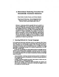
all the implicit features between a concept and its sub-concept will be stored in a single edge. This could potentially limit the concept representation, and thus limit OF’s inference process. Moreover, hierarchical clustering algorithms used in Algorithm 1 always select the best cluster to merge/split based on the optimization of one of the criterion function in Table 1. Thus, it ignores other possible suboptimal candidates. In the next section, experimental results show that, on average, it is the agglomerative clustering with the complete-link criterion function that achieves the best result. Algorithm 3 extends this algorithm in order to build multi-hierarchical ontologies. Algorithm 3 Learning a Multi-Hierarchical Ontology with a window size α and threshold cluster θ Input: A set of items I, and the similarity matrix S, α, and θ. Output: a clustering tree modeling a multi-hierarchical ontology. 1. C ← φ 2. Assign each item i to its own cluster Ci and C = C ∪ Ci . 3. while |C| > θ do 4. X ← φ 5. For each Ci , Cj in C do 6. X ← X ∪ (xCi ,Cj = mini∈Ci ,j∈Cj sim(i, j)) 7. xCi ,Cj ← max(X) 8. Ck ← merge(Ci ,Cj ) 9. Cm ← {Ci , Cj } 10. C ← C/Cm 11. window ← xi,j − αxi,j ; X ← φ 12. For each Cp in Cm , Cq in C do 13. xCp ,Cq ← minp∈Cp ,q∈Cq sim(p, q) 14. if xCp ,Cq > window then 15. Cr ← merge(Cp ,Cq ) 16. C ← C ∪ Cr 17. C ← C ∪ Ck
Clu ste Ag glo me rat ive
Cr
step 8
step 15
Cj
Cq
Cj=Cp step 6 - xci,cj
Agglomerative clustering with clink C={Ck, Cq} And with Step 11->16 C={Ck, Cr, Cq}
6 ->1 11
Ck
ps Ste
rin gw it h
clin k
The first 10 steps and the step 17 of Algorithm 3 are in fact the classical agglomerative clustering with the complete-link criterion function, where the complete-link criterion function is being used in step 6. Given a coefficient α ∈ [0..1] as input parameter, step 11 computes a window size of acceptable clusters based on the value of the criterion value and α. Given this window size, we look at all the possible pairs of clusters that can be made with one of the merged cluster Ci or Cj , and see if its criterion value is within the window size. For each of these pairs, we merge them into a unique cluster and add it to the list of open clusters C. Notice that xCp ,Cq cannot be bigger than xCi ,Cj as the pair Ci Cj optimizes the criterion function in step 6. As cluster Cp has a already got a parent (i.e.: Ck ), step 15 makes cluster Cr another parent of Cp .
ments on two famous data sets: MovieLens1 and Jester2 . MovieLens is the most famous data set in the recommendation system community; it contains the ratings of 943 real users on at least 20 movies. There are 1682 movies in total, which can be described by 19 themes: drama, action, and so forth. Jester is another famous data set that contains the users’ ratings on jokes collected over a period of 4 years. The data set contains over 4.1 Million ratings and is actually split into three zip files: jester-data-1.zip, jester-data-2.zip, jester-data-3.zip. In this paper, we only used the first data set; it contains already 24,983 users on all the 100 jokes. These sets were used for three reasons. First and most importantly, they are the most widely used data sets, which makes it easy to reproduce the experiments. Second, both of those data sets contain (real) rated items which are necessary for filling in the useritem matrix R. Finally, these sets are very different in content and sparsity, where the sparsity is defined as the fraction of entries in the matrix R without values [10] over the total number of possible entries. For example, MovieLens contains movies that can easily be defined with some features such as the theme, duration, and so forth. However, Jester is made up of jokes, which is much harder to describe and thus is an ideal candidate to test our ontology learning algorithm. Notice also that the sparsity of MovieLens(0.937) is much greater than the one of Jester(0.447). The experiment set up was as follows. First, we selected all the users who rated at least 65 items, and used the remaining one to populate the user-rating matrix R. After removing users with less than 65 ratings, we are left with 407 users in MovieLens and 6199 users for Jester. For each remaining user, we randomly separated its ratings into two non-overlapping sets IS and T S. The intermediate set IS contains exactly 50 ratings, while the set T S contains the remaining ratings. The intermediate set IS is used to study the behavior of the recommendation algorithms with different amounts of rating data to learn the model. In the first case, we extracted 5 ratings from IS that we put into a learning set LS, in order to simulate the case when few preferences about the user are known. In the other situation, we used all 50 ratings in IS to see how the algorithms behave when a lot of ratings are available for learning the model. The testing set T S is used for computing the prediction using the top-N recommendation policy, with N set to 5. For these experiments, we used the toolkit CLUTO3 version 2.1.1 that implements all of the partitional and agglomerative clustering algorithms used by Algorithm 1. For the COBWEB algorithm, we used the java package WEKA4 version 3.4.
4.1
P recision =
Step 13 - xcp,cq
Figure 3: Illustration of Algorithm 3
1
EXPERIMENTS To evaluate our algorithms, we performed two identical experi-
Nok Nok ; Recall = |RS| Nr
http://www.cs.umn.edu/Research/GroupLens/data http://www.ieor.berkeley.edu/∼goldberg/jester-data/ 3 http://glaros.dtc.umn.edu/gkhome/cluto/cluto/download 4 http://www.cs.waikato.ac.nz/∼ml/weka/ 2
4.
Evaluating Recommendation Algorithms
Many metrics have been proposed for evaluating the accuracy of the predictions made by recommendation systems. The most famous metric used to be the Mean Absolute Error, (MAE, [10]), which evaluates the accuracy by measuring the mean average deviation between the expected rating and the true rating. Later on in [5], it was argued that this metric was in fact not very accurate when considering rated items for users, as a user is usually interested to know if he’s going to like the item or not. As a consequence, [5] proposed to use the classical information retrieval metrics: precision and recall. Given a recommendation set RS, precision is defined as the ratio of relevant items Nok by the total number of items shown in RS, while recall is defined by the ratio of relevant items to the total number of relevant items available in the database, Nr . (7)
There are two challenges when using precision and recall for evaluating the accuracy of recommendation systems. First, precision and recall need to be considered as a whole to fully evaluate the performance. Second, it has been observed in many applications that precision and recall are in fact inversely related. Thus, we need to use a metric that is able to combine both precision and recall. As a consequence, and following the results in [5], we use the F1 metric to evaluate the accuracy of a recommendation system. This metric combines the precision and recall into a harmonic mean ranging from 0 to 1, where 0 occurs when both precision and recall are null. Inversely, the value 1 only happen if both precision and recall are both equal to 1. Formally, the F1 metric is defined as follows: F1 =
2P recision ∗ Recall P recision + Recall
(8)
The main objective of our learnt ontologies is to help recommender systems to correctly recommend items. Thus, we will also use the F1 measure on the recommended items to evaluate the quality of the learnt ontologies.
4.2
Hierarchical Clustering Analysis
In this experiment, we studied the behavior of the ontologies generated by Algorithm 1, and their efficiency as ontologies in the personalized ontology filtering approach. Following Algorithm 1, we analyzed all the possible combinations made by the criteria functions given in Table 1. Thus, we obtained 15 different ontologies: 6 using the partitional approach, and 9 with the agglomerative approach. Given these ontologies, we implemented pOF with Algorithm 2 to see whether or not the ontology personalization helps to increase the prediction accuracy. Note that the COBWEB algorithm was use to benchmark the learnt ontologies. Table 2 summarizes the various algorithms used in this experiment. Table 2: Notations used by the various algorithms P i1 P i2 P e1 P g1 P h1 P h2 A i1 A i2 A e1 A g1 A h1 A h2 A slink A clink A upgma COBWEB pOF
Partitional clustering using criterion I1 Partitional clustering using criterion I2 Partitional clustering using criterion E1 Partitional clustering using criterion G1 Partitional clustering using criterion H1 Partitional clustering using criterion H2 Agglomerative clustering using criterion I1 Agglomerative clustering using criterion I2 Agglomerative clustering using criterion E1 Agglomerative clustering using criterion G1 Agglomerative clustering using criterion H1 Agglomerative clustering using criterion H2 Agglomerative clustering using criterion slink Agglomerative clustering using criterion clink Agglomerative clustering using criterion UPGMA The concept-based clustering algorithm Personalized ontology filtering(Algorithm 1 & 2)
Each learnt ontology was then fed as input ontology to the ontology filtering algorithm, and prediction on all the users were made. To measure the quality of the ontologies, we used the prediction accuracy defined in Equation 8 (i.e.: the F1 metric). The underlying assumption is that a good ontology should generate good recommendations, and thus increase the prediction accuracy. The results obtained by the different criteria functions significantly diverge within the same family of algorithms (i.e.: partitional or agglomerative). As a consequence, we thought that using a simple average measure over all the criteria would induce too much bias. Especially when we consider the fact that there are more agglomerative algorithms than partitional. To simplify the understanding,
we transformed the F1 results into relative F1 value, rF 1. This is done by dividing the F1 results by the maximum possible value between the 15 possible ontologies. Notice that the relative F1 value is very similar to the relative Fscore introduced in [15]. To have a better understanding of the behavior of each ontology, we tested it with different numbers of leaf clusters, ranging from 5 to the number of items available. Notice also that such a detail study was not performed by [15]. #clusters P-i1 P-i2 P-e1 P-g1 P-h1 P-h2 A-i1 A-i2 A-e1 A-g1 A-h1 A-h2 A-upgma A-slink A-clink pOF COBWEB
5 0.92373 1 0.72432 0.66714 0.95538 0.96416 0.9235 0.93752 0.79454 0.66714 0.74057 0.84804 0.93958 0.66677 0.95016 1.07357 0.70159
10 0.97397 0.99023 0.69181 0.72318 1 0.97633 0.94892 0.9719 0.73172 0.72394 0.83112 0.85124 0.98224 0.68665 0.9561 1.10116 0.69947
20 1 0.98308 0.78296 0.74148 0.92673 0.93697 0.97217 0.98335 0.667 0.77269 0.76735 0.80934 0.95688 0.70083 0.95704 1.07586 0.66771
40 0.98208 0.98267 0.79208 0.90908 0.89358 0.87226 0.95752 0.92592 0.66709 0.90744 0.79804 0.73035 0.96617 1 0.97443 1.0788 0.64461
60 0.92791 0.90027 0.76153 0.97757 0.91473 0.78784 0.93228 0.88596 0.70788 1 0.82775 0.84645 0.93888 0.99565 0.95343 1.05005 0.62035
80 0.8884 0.90149 0.75762 0.99919 0.87 0.81062 0.89474 0.84463 0.80379 1 0.83622 0.87914 0.89702 0.96017 0.88577 0.9517 0.6091
100 0.89714 0.85413 0.84822 1 0.85138 0.85169 0.89714 0.87532 0.84534 0.97004 0.8558 0.90457 0.88038 0.97172 0.89153 0.91722 0.63131
Avg 0.94189 0.94455 0.76551 0.85966 0.91597 0.8857 0.93233 0.9178 0.74534 0.86303 0.80812 0.83845 0.93731 0.85454 0.93835 1.03548 0.65345
Figure 4: Relative F1 values for Jester, 5 ratings in LS Figure 4 and 5 display the relative F1 values obtained on the Jester data set. First, we can see that on average, pOF using Algorithm 2 to select the best learnt ontology performs better than any of the simple clustering algorithms (rF 1 = 1.0355 and rF 1 = 1.0469), whatever the size of the learning set. This tends to confirm our intuition that not one ontology is strictly better than the others, but rather that some users will reach a better accuracy with a given ontology. Notice that having a relative score superior to 1 for pOF is not a mistake. It is due to the fact that the maximum is computed on the 15 simple clustering ontologies only. Another important result is that the ontology learnt by COBWEB is the worst performing ontology. The main reason for this lies in the definition of COBWEB: it is a conceptual clustering algorithm. As a consequence, items need to be defined by a set of attribute-value pairs. In our E-commerce context, this data is unavailable as we only have the user-matrix R. This is also an indication that the technique [1] of transforming the item-to-item similarity matrix into attribute-value pairs is not suitable in this domain. When 5 items are used for learning the user’s score, the partitional clustering with the i2 criteria function (P-i2) has the best average relative score. Then, partitional clustering with the h1 function (P-h1) becomes the best algorithm when 50 items are used for learning the data set. This tends to go in the direction of Zhao’s conclusions [15] that partitional clustering algorithms perform better than agglomerative ones. Notice the evolution of the clustering P-g1 with the number of clusters. If only very few clusters are created, then P-g1 performs badly. However, when we have many clusters, P-g1 performs really well which tends to show that the graph criterion requires many leaf clusters to generate a good ontology. When the number of clusters are set to either 40, 60, 80, and LS to 5, then interestingly agglomerative algorithms do perform better than partitional clustering ones. This would indicate (and the results with MovieLens confirm this) that agglomerative clustering needs enough leaf clusters to perform correctly, while partitional algorithm seems better with less clusters. It makes sense when we consider the fact that partitional algorithms are top down approaches that recursively split clusters. Thus, too many splits may degrade the ontology, as it generally increases the variance. Inversely, agglomerative clusterings are bottom up approaches that recursively merge clusters. When looking at the MovieLens data set (Figure 7 and 8), we
Jester MovieLens
#clusters P-i1 P-i2 P-e1 P-g1 P-h1 P-h2 A-i1 A-i2 A-e1 A-g1 A-h1 A-h2 A-upgma A-slink A-clink COBWEB 100 0.247922 0.264556 0.271966 0.435304 0.469359 0.531173 0.198463 0.21052 0.21581 0.219471 0.33306 0.360501 0.197228 0.195981 0.196595 0.751616 1682 147.4204 185.8118 196.6213 120.7714 1293.98 1592.284 34.79125 35.89776 37.59519 33.97908 694.5894 835.5383 36.59017 37.22639 33.58081 30816
Figure 6: Execution time in seconds required for the clustering algorithm to generate the ontology. #clusters P-i1 P-i2 P-e1 P-g1 P-h1 P-h2 A-i1 A-i2 A-e1 A-g1 A-h1 A-h2 A-upgma A-slink A-clink pOF COBWEB
5 0.92199 1 0.86218 0.59848 0.98554 0.94253 0.98182 0.95756 0.90571 0.59848 0.72858 0.83612 0.9528 0.60301 0.99592 1.10507 0.64866
10 1 0.94498 0.77141 0.62347 0.99668 0.98046 0.96576 0.97014 0.8353 0.62783 0.76684 0.8311 0.92766 0.60367 0.96524 1.08234 0.64406
20 0.9502 0.9513 0.6962 0.6806 1 0.96519 0.92109 0.92747 0.61178 0.68842 0.71589 0.76491 0.92468 0.63717 0.95768 1.05344 0.63953
40 0.92113 0.93071 0.81741 0.82298 1 0.95347 0.9156 0.90997 0.59828 0.81516 0.73853 0.68172 0.96043 0.97247 0.92494 1.05072 0.63206
60 0.94957 0.92297 0.71435 0.97371 0.95368 0.9027 0.94747 0.91396 0.64679 0.95787 0.7958 0.81398 0.95605 1 0.95371 1.05502 0.62773
80 0.89892 0.91032 0.72781 1 0.86795 0.84852 0.89915 0.92123 0.76108 0.9641 0.81557 0.86419 0.91222 0.92229 0.90206 1.02225 0.62337
100 0.94203 0.90704 0.89892 0.89384 0.90357 0.90338 0.94203 0.96367 0.90683 0.94361 0.92598 1 0.9804 0.9835 0.96859 0.95915 0.69863
Avg 0.94055 0.93819 0.78404 0.79901 0.9582 0.92803 0.93899 0.93771 0.75225 0.79935 0.78389 0.82743 0.94489 0.81744 0.95259 1.04686 0.64486
#clusters P-i1 P-i2 P-e1 P-g1 P-h1 P-h2 A-i1 A-i2 A-e1 A-g1 A-h1 A-h2 A-upgma A-slink A-clink pOF COBWEB
5 0.85819 0.77527 1 0.86951 0.94444 0.91684 0.52208 0.64579 0.58947 0.56556 0.83433 0.9038 0.72438 0.52469 0.90848 1.26798 0.71347
20 0.90691 0.92806 0.94035 0.87643 1 0.846 0.51313 0.58586 0.52755 0.58262 0.89713 0.90267 0.65738 0.47677 0.92253 1.34464 0.63978
60 0.93299 0.97378 0.92338 0.91947 1 0.89171 0.53684 0.62117 0.55189 0.66565 0.90878 0.90827 0.68674 0.5641 0.92626 1.34023 0.67423
100 0.89813 0.89361 0.88621 0.89565 0.92986 0.86179 0.49868 0.601 0.51796 0.70807 0.91827 0.91641 0.66053 0.53024 1 1.35016 0.65088
500 0.86582 0.88676 0.72445 0.88505 0.96069 0.84053 0.47846 0.59558 0.84788 0.74149 0.91451 0.85527 0.64499 0.47789 1 1.27567 0.64279
1000 0.87823 0.86677 0.68143 0.79018 0.9099 0.71635 0.80507 0.8178 1 0.79567 0.79441 0.76771 0.84773 0.69957 0.79018 1.19754 0.55043
1682 0.8595 0.86777 0.68595 0.78512 0.90909 0.72727 0.80992 0.80165 1 0.78512 0.78512 0.75207 0.82645 0.67769 0.77686 1.06612 0.91736
Avg 0.88568 0.88458 0.83454 0.8602 0.95057 0.82864 0.59488 0.66698 0.71925 0.69203 0.86465 0.85803 0.72117 0.56442 0.90347 1.26319 0.68414
Figure 5: relative F1 score for Jester, 50 ratings in LS
Figure 8: Relative MovieLens Jester, 50 ratings in LS
can see that the results are very similar than the one obtained with Jester. For example, personalized ontology filtering performs better on average than any of the clustering algorithms taken separately, whatever the size of the learning set LS. As a mater of fact, the improvement is even more significant than with Jester. Second, the ontology produced by COBWEB is again giving a very poor prediction accuracy. For the first time, the agglomerative clustering with the clink criteria function is the best performing clustering algorithm when 5 items are used for learning the user’s model. Note however, that P-i1 is nearly as good as A-clink, and thus no clear conclusion can be drawn from this result.
another. The worst performing algorithm is COBWEB, which requires nearly 9 hours to come up with a clustering tree on MovieLens! We expected such a result as the complexity is exponential to the number of attribute-value pairs, which in the case is equal to 1682 different items (attribute) and two values (good or bad). As a consequence, COBWEB clearly does not scale well to big problems. However, it is good to point out that this computation can be broken into smaller parts, as COBWEB is an incremental algorithm. Very surprisingly, agglomerative clusterings took less time to compute than partitional clusterings, which is obviously not what is expected when reading the general literature. This is not a mistake, and there are two explanations for this. First, the most expensive step in agglomerative clustering is the pairwise similarity computation of all the pairs of items. In our situation, the matrix S containing this data has already been computed, and thus remove this O(n2 ) step. Second, as highlighted by Zhao[15], the pair-wise similarities or the improvements in the value of the criterion function achieved by merging a pair of clusters i and j do not change during the different agglomerative step, as long as i and j is not selected to be merged. Finally, using the criteria functions H1 and H2 significantly increases the execution time of the clustering algorithm. These results are coherent with the theory as H1 and H2 are both hybrid functions that respectively combine criteria I1 with E1 , and I2 with E1 .
#clusters P-i1 P-i2 P-e1 P-g1 P-h1 P-h2 A-i1 A-i2 A-e1 A-g1 A-h1 A-h2 A-upgma A-slink A-clink pOF COBWEB
5 0.84069 0.87627 0.90203 0.9193 0.9281 0.8758 0.72539 0.85194 0.7468 0.74558 0.88115 1 0.87567 0.72786 0.89295 1.20871 0.82724
20 0.91926 0.79532 0.83749 0.87733 1 0.82128 0.64607 0.74609 0.65229 0.67179 0.91094 0.88216 0.76542 0.63624 0.91503 1.20327 0.72471
60 0.98805 0.79741 0.68534 0.72397 0.79987 0.67032 0.5235 0.61221 0.52695 0.55442 0.75327 0.77272 0.62262 0.52852 1 1.18411 0.59
100 0.93512 0.74341 0.64131 0.68421 0.73797 0.62582 0.4808 0.57204 0.4808 0.53726 0.79041 0.83676 0.58107 0.4808 1 1.09918 0.55166
500 1 0.8143 0.68346 0.82052 0.99298 0.70004 0.50637 0.58314 0.74603 0.67057 0.8596 0.86767 0.61131 0.50637 0.98353 1.20731 0.58101
1000 1 0.97471 0.63691 0.88072 0.9237 0.69636 0.91393 0.89917 0.84548 0.90855 0.83508 0.82843 0.91952 0.61383 0.93932 1.07737 0.52325
1682 0.98595 0.87408 0.89353 0.88207 0.81748 0.79924 1 0.90802 0.80962 0.82148 0.70466 0.74439 0.95968 0.90483 0.96958 0.80673 0.50779
Avg 0.95272 0.83936 0.7543 0.82687 0.88573 0.74127 0.68515 0.73894 0.68685 0.70138 0.8193 0.84745 0.76218 0.62835 0.9572 1.11238 0.61509
Figure 7: Relative F1 values for MovieLens, 5 ratings in LS When 50 ratings are used in LS, the best performing ontology is again the one learnt using the partitional clustering with the H1 function. This tends to suggest that, on average and when sufficient data about the user is known, partitional clustering with the H1 criteria function performs the best. A detailed analysis of the ontology size reveals in fact that the agglomerative clustering with the clink function can outperform P-i1 if the number of clusters are set to either 100 or 500. Fortunately, our pOF approach with Algorithm 2 is capable of predicting which ontology to use as its relative F1 score is always bigger than 1, and whenever the number of clusters are less or equal to 1000. When considering which clustering algorithm to use, the accuracy of the prediction should not be the only criterion. The execution time required to build the tree should also be an important aspect. In Figure 6, we indicated the execution time (in seconds) required for the clustering algorithm to generate its tree. As expected, the execution time does vary a lot from one algorithm to
4.3
Multi-Hierarchical Clustering Analysis
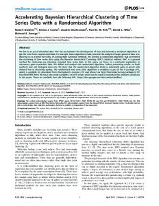
In this experiment, we wanted to see whether the multi-hierarchical ontology generated by Algorithm 3 does increase the recommendation accuracy or not. To test this aspect (and due to the limited amount of space) we only reproduced the Jester experiment, and compared it with the behavior of the agglomerative clustering using the clink criterion function. First, we looked at the number of extra clusters generated by the step 11 to 16 of Algorithm 3. As expected, the dotted line in Figure 9 shows that by increasing the coefficient α, many extra clusters are being created. Notice that following algorithm 3, one extra cluster implies that 2 clusters will have at least 2 parents. An interesting aspect is to consider whether keeping increasing the size of the window will always improve the accuracy of the recommendation. The plain line in Figure 9 shows the average accuracy of the recommendation made by using Algorithm 3 for generating the ontology. The average accuracy was obtained by averaging the F1 values when respectively using 5, 10, 20, 40, 60, 80, and 100
4.4
90 Number of extra clusters generated by step 11 to 16 of Algorithm 3 80
Scaled accuracy of recommendation of Algorithm 3
70 60 50 40 30 20 10 0 0.15
0.2
0.25
0.3
0.35
0.4
0.45
0.5
alpha
Figure 9: Number of extra clusters generated by Algorithm 3 leaf clusters in the ontology. Note also that the F1 metric values were scaled up to fit in the interval 0 to 90 by using the formula y = 3000 ∗ F 1value − 900. The solid line clearly indicates that increasing the window size leads to better prediction accuracy. However, if the window becomes to big (i.e. α > 0.4), then the structure becomes overloaded by inheritance edges, which significantly increases the search space. Finally, notice that increasing the coefficient α will also increase the computational resources required to build the ontology. Thus, a tradeoff will need to be done between prediction accuracy and ontology quality. In Figure 10, we plotted the prediction accuracy obtained using the ontology filtering approach with different learning sets sizes. The plain line is ontology filtering using Algorithm 3 to build the ontology, while the doted line is OF that uses the classical agglomerative clustering with clink for the ontology construction. This is respectively represented by the Algorithm 3 * and A clink * and lines, where ∗ is the size of the learning set for learning the scores.
Recommendation Accuracy
The first experiment showed that our personalized ontology filtering led to the best results compared to classical clustering algorithms. Following these results, we focus on whether our personalized ontology filtering approach is in fact better or worse than collaborative filtering. For the experiments, we analyzed the item-based collaborative filtering (CF) using the adjusted cosine similarity for the similarity between pairs of items, and the personalized ontology filtering (pOF) defined in section 3.2. CF was used as benchmark as it is the most widely used recommendation system. For the ontology filtering, we used Algorithm 1 to generate all the ontologies, and used Algorithm 2 to select the best ontology to be used by each user. The performance of CF greatly depends on the number of neighbors used to compute the prediction (Equation (2)). At the same time, the ontologies generated by Algorithm 1 will be different depending on the number of leaf clusters (i.e.:threshold θ) that were specified. To test these aspects, we ran the algorithms using various values of leaf clusters and neighbors. Figure 11 shows the accuracy of the pOF and CF recommendation systems on the Jester data set. The dashed lines represent collaborative filtering, while the plain lines are the personalized ontology filtering. The notation *-5LS and *-50LS means that 5 and respectively 50 items were used to learn the model. The xaxis shows the number of neighbors that were used for CF, which is also the same parameter used for the number of leaf clusters in Algorithm 1. The y-axis measures the accuracy of the recommendation using the F1 metric. 0.4 CF_5LS pOF_5LS 0.38
CF_50LS pOF_50LS
F1 Metric
0.36 0.39
0.34
0.37
0.32 0.35
F1 Metric
0.3 0.33
0.28 10
0.31
20
40
60
80
100
#clusters/neighboors 0.29 Algorithm 3_5LS A-clink_5LS
0.27
Algorithm 3_50LS A-clink_50LS
0.25 5
10
20
40
60
80
100
#leaf cluster in the learnt ontology
Figure 10: Accuracy for the Jester data set, with α set to 0.4 These results tend to go in favor of our hypothesis, which states that a multi-hierarchical structure leads to a better ontology than a simple hierarchical one. As one can see, the ontology generated with the multiple inheritance algorithm reaches nearly always the best prediction accuracy, with the best improvements when the ontology contains at least 80 leaf clusters. When using agglomerative clustering with the clink criterion function, the prediction accuracy fluctuates up and down depending on the parameter number of leaf clusters, and significantly decreases when the ontology contains 100 leaves. This unwanted behavior is not observed with the multiple inheritance algorithm, which seems more robust to the number of leaf clusters. This can be explained by the fact that Algorithm 3 builds many extra inheritance edges, which means that the inference process has a higher probability of finding a shorter path between two given concepts. This shorter path will allow more score to be transferred between these concepts, which leads to a better inference process.
Figure 11: Accuracy for the Jester data set First, and most important, we can see that ontology filtering using the learnt ontologies performs much better than CF. The result is even more emphasized when very few ratings (only 5, OF-5LS) are used to learn the model. As a matter of fact, the improvement of our personalized OF is always significant (p-value