Hierarchical Correlation Compensation for Hidden Markov Models

HIERARCHICAL CORRELATION COMPENSATION FOR HIDDEN MARKOV MODELS Hui Lin*, Ye Tian**, Jian-Lai Zhou**, Hui Jiang*** *Dept. of Electronic Engineering, Tsinghua University, Beijing, China ** Microsoft Research Asia, Beijing, China *** Dept. of Computer Science and Engineering, York University, Canada Email: [email protected]; {t-yetian,jlzhou}@microsoft.com; [email protected] ABSTRACT In this paper, we present a Hierarchical Correlation Compensation (HCC) scheme to reliably estimate full covariance matrices for Gaussian components in CDHMMs for speech recognition. First, we build a hierarchical tree in the covariance space, where each leaf node represents a Gaussian component in the CDHMM set. For all lower-level nodes in the tree, we estimate a diagonal covariance matrix as usual. But we estimate full matrices for all upper-level nodes since they have large amount of data. For each Gaussian in a leaf node (with diagonal components estimated already), we compensate its offdiagonal components by using a linear combination of a set of prototype covariance matrices, which includes the estimated covariance matrices of all nodes in the tree along the upward path from the leaf all the way to the root. At last, the linear combination weights are estimated based on the maximum likelihood (ML) criterion. We have evaluated the HCC on the DARPA Resource Management (RM) task and an in-house large-vocabulary Chinese dictation task. We have achieved significant error reduction over the best diagonal covariance models. Experimental results also show that HCC yields better performance than other full covariance modeling schemes.

1. INTRODUCTION Full covariance explicitly models the correlation among feature components. But it is very difficult to obtain reliable estimation of a full covariance matrix due to a large number of free parameters to be estimated in practice. In speech recognition based on CDHMMs, we usually adopt diagonal covariance matrices for all Gaussian components in the models. Diagonal covariance matrix implies strong assumption that the feature components are independent. Even mixtures of diagonal covariance can model the correlation to some extent; the model precision is still limited. In speech recognition, many different approaches have been proposed to de-correlate feature dimensions for this purpose in either feature or model space. In feature space, it is well known that Discrete Cosine Transform (DCT) [2] and Linear Discriminant Analysis (LDA) [3] are used in the front-end processing. In model space, Maximum Likelihood Linear Transform (MLLT) [4] and Heteroscedastic Linear Discriminant Analysis (HLDA) [5] use a global projection matrix optimized by the maximum likelihood criterion. Besides, semi-tied Covariance (STC) [6] and Multiple HLDA (MHLDA) [7] also address the same issue by building multiple subspace projections.

0-7803-8874-7/05/$20.00 ©2005 IEEE

Recently, people have proposed several approaches to directly estimate full precision matrices in CDHMMs based on a linear combination of a set of global prototype full precision matrices, such as mixture of covariance (MIC)[8], SPAM[9], modeling covariance by basic expansion [10]. Experimental results show that all these full precision modeling approaches outperform the diagonal models. In this paper, we present a Hierarchical Correlation Compensation (HCC) method to reliably estimate the full covariance matrices in CDHMMs based on a tree-based prototyping scheme. First of all, we build a hierarchical tree in the covariance space, where each leaf node represents a Gaussian component in the CDHMM set. For all lower-level nodes in the tree, we estimate a diagonal covariance matrix as usual. But we estimate full matrices for all upper-level nodes since they have large amount of data. For each Gaussian in a leaf node (with diagonal components estimated already), we compensate its off-diagonal components by using linear combination of a set of prototype off-diagonal covariance matrices, which includes the estimated covariance matrices of all nodes along the upward path from the leaf all the way to the root in the tree. At last, the linear combination weights are estimated based on the maximum likelihood (ML) criterion. We have evaluated the above HCC algorithm on the RM database and an in-house large vocabulary Chinese dictation task, experimental results shows that our HCC algorithm yields better performance than all other existing full covariance modeling methods, such as STC, HLDA, and MIC. The remainder of this paper is organized as follows. In section 2, we give the outline of our algorithms, followed by hierarchal tree build in section 3. The hierarchal correlation compensation scheme is described in section 4. The experiments are reported in section 5 and 6. Finally, we conclude the paper with our findings in section 7.

2. THE HCC ALGORITHM OUTLINE Our hierarchical covariance compensation (HCC) scheme consists of the following five steps: 1. Train a baseline model set of tri-phone CDHMMs with diagonal covariance matrices. The mean and the covariance are estimated as usual based on the ML criterion. We will keep the structure, mixture weights, and the mean vectors of the baseline model set unchanged in following stages. 2. All the tied-states are used to build a tree. The tree can be built according to the full covariance’s K-L distance with

I - 673

ICASSP 2005

the top-down clustering. Or we can use the decision tree generated from the previous baseline model training stage. We use tied-states as base elements in tree-building since the full covariance matrices of Gaussian components may not be reliable for the clustering. After the tied-state tree is built, for each tied-state node we expand all its Gaussian components as another layer of its child. Estimate a covariance matrix for each node in the tree. For all leaf nodes, we estimate diagonal covariance matrices. For each upper-level node, a full covariance matrix is estimated from all of its child nodes. For each Gaussian component in a leaf node, the estimated full covariance matrices of all the nodes along the upward path from the leaf node to the root are used to estimate the off-diagonal components in its full covariance matrix based on a linear combination scheme, where the combination weights are estimated by the maximum likelihood criterion. Replace the diagonal covariance matrices in the model set trained in step 1 with the newly estimated full covariance matrices. The resultant model set is used for recognition.

4.

5.

¦ node

¦

¦

…

…

…

¦ node

…

3.

¦ root

tied − state

m

Figure 1. The tree generated from the top-down covariance matrix clustering

i th tied-state node is ω tied − state ,i =

The weight of

¦ω

m {components ∈ ith tied − state}

3. HIERARCHICAL TREE BUILDING To build a tree, we use the tied-states in the baseline model as basic elements. There are two ways to build the tree. The first one is to use the covariance matrices’ K-L distance measure to do the top-down matrix clustering. The second one is to derive from the decision trees generated in the baseline model training stage.

(5)

We then use all the tied-state nodes to do the top-down clustering as in [11]. In clustering, we need to define how to calculate distance measure between each pair and how to compute a center for each new cluster. The distance measure between two Gaussian densities

(

g m ( x) = N x; µ m ; ¦ −m1

) and

(

g n ( x) = N x; µ n ; ¦ −n1

)

is defined as the sum of the Kullback-Leibler (KL) divergence 3.1 Top-down covariance matrix clustering In the training process, we use maximum likelihood to estimate the mean vectors and full covariance matrices of each Gaussian component. The mean of the m ’th Gaussian component

from

g m ( x)

g n ( x)

−1 m

−1 n

to

)

g m ( x) . That is

T

+ (µ m − µ n ) ¦ n−1 (µ m − µ n ) (1)

m

m ’th Gaussian component

Since only the covariance is of interest, the distance between the Gaussian means is ignored. Eventually, we use the following formula to calculate the distance between two covariance matrices:

(

d (m, n) = Tr ¦ −m1 ¦ n + ¦ −n1 ¦ m

is

Σm =

¦τ γ

m

(

)(

(τ ) ο (τ ) − µ m ο (τ ) − µ m

¦τ γ

m

,where ο (τ ) is the τ ’th observation vector;

We define the

)

T

(2)

(τ )

probability that ο (τ ) belongs to the

γ m (τ )

is the

¦ node,k =

m ’th component’s weight ω m as (3)

τ

The full covariance matrix of the i th tied-state node i is estimated from all of its child nodes as:

¦ tied − state ,i =

¦

m m { m∈ith tied − state ' s components}

¦ω

m { m∈ith tied − state ' s components}

¦ [ω

i∈G ( k )

tied − state , i

¦ω

i∈G ( k )

ω m = ¦ γ m (τ )

.

(4)

)

(7)

Next, for each intermediate node k in the tree, a full covariance matrix is calculated from all tied-states belonging to the node k as:

m ’th Gaussian component.

¦ω

(6)

T

¦τ γ (τ )ο (τ ) = ¦τ γ (τ )

The full covariance matrix of the

(

and from

+ (µ n − µ m ) ¦ m−1 (µ n − µ m )

m

Σm

g n ( x)

d (m, n) = Tr ¦ ¦ n + ¦ ¦ m

µ m is µm

to

,where

G (k )

¦ tied − state , i ]

(8) tied − state , i

is the set of all the elements belonging to node

k . ω tied − state , i and ¦ tied − state , i are

the weight and the full

covariance matrix of tied-state. Based on the distance measure in Eq. (7) and new center calculation in Eq.(8), we use the standard top-down clustering approach to build the tree and expand each tied-state in leaf node with all its Gaussian components as shown in Figure 1.

I - 674

3.2 Phonetic decision tree based tree building Different from the previous top-down clustering tree, the data is initially divided into monophone clusters. Then each monophone’s node is expanded with its phonetic decision trees generated in baseline model training for this monophone. The leaf nodes up to this point are all tied-states. Then each leaf node is expanded with all its Gaussian components as another layer of child nodes. The resultant decision tree is shown in Figure 2. The full covariance matrix of each intermediate node is estimated based on Eq. (8).

M

[

(

ˆ −1 − Tr ¦ ˆ −1 ¦ Q(Λ ) = ¦ ω i log ¦ i i i i =1

is the component’s weight defined in Eq. (3).

i

is the new full covariance matrix to be estimated as in Eq.(10), where only the weights

λi ,m are

For each Gaussian component

¦ node

…

Layer 2 (monophone)

Decision Tree

¦ node

……

Layer 3

unknown.

M is the total

……

i

, the weights

¦ node

……

Leaf nodes (Gaussian Component)

¦

…

……

(

…

4.1 Linear combination Assume a Gaussian component in the i th leaf node, all intermediate nodes along the upward path from this node to the root is defined as the set:

­ i ' s parent , i ' s parent' s parents Ψ (i ) = ® ¯....,..., root

ˆ ¦ i

of the

i

,½ ¾ ¿

th Gaussian

, where

diag (¦ i )

i ,m

node , m

− diag (¦ node,m )

m∈Ψ ( i )

].

(10) is the diagonal matrix of

¦i ,

and λi, m

are all combination weights to be estimated. 4.2 Weight estimation The linear combination weights

λi,m

5. EXPERIMENTS (I): THE RM TASK In this section, the above HCC method is evaluated in the DARPA RM task. A total of 3990 sentences are used for training and the baseline model is trained by using HTK which starts from a single Gaussian monophone system. After four iterations of embedded training, the monophone models are cloned to produce a single Gaussian triphone system. In-word triphone models are used in our experiments. These initial triphone CDHMMs are trained with two iteration of embedded training after the decision-tree tying. The baseline system in step 1 is produced by standard iterative mixture splitting using four embedded training per mixture increasing. At last, 6 Gaussian mixture components with diagonal covariance matrices are trained as the baseline model for each tied-state. A total of 1199 sentences are used as the test data. The decoding is based on HTK which uses a word-pair grammar. The word error rate (WER) of the baseline system is 4.09%.

(9)

components is estimated by

¦ λ [¦

(12)

weights λi, m in the Matlab® optimization toolbox.

4. HIERARCHICAL CORRELATION COMPENSATION In the baseline model set, all diagonal components in covariance matrices are estimated reliably. Only off-diagonal components are needed to be compensated. For each Gaussian component, all the nodes along the upward path to the root are used to estimate the off-diagonal components for this Gaussian component based on a linear combination strategy. The linear combination weights are estimated by the maximum likelihood criterion.

ˆ = diag (¦ ) + ¦ i i

)

N mixture components

Figure 2. Tree structure generated from phonetic decision trees

Thus the new full covariance

are

We use a numerical method to maximize the Q function w.r.t.

…

m

λ(i )

independent from other Gaussian components. Hence the optimization problem of the whole model can be decomposed into M small optimization problems. That is, for i = 1,2..., M , optimizing

ˆ −1 − Tr ¦ ˆ −1 ¦ Q (Λ i ) = log ¦ i i i Layer K (Tied-state state)

(11)

¦ i is ˆ i th component’s full covariance estimated as in Eq.(2). ¦

, where the

ωi

)]

number of Gaussian components in the model set.

¦ root

Layer 1 (root)

component. The EM algorithm is used here. The auxiliary function in the EM algorithm can be written as

are estimated to maximize

the likelihood function of data belonging to this Gaussian

5.1 Compared with other related techniques First of all, we compare the HCC with other existing related techniques, such as HLDA[5], STC[6], and MIC[8]. The result is shown in table 1. From the table, we can see that all the techniques can achieve better performance than the baseline model set with diagonal covariance matrices. Among all these techniques, the HCC gives the best performance and the relative WER reduction is up to 22.7%. The reason is that after we successfully overcome the reliable estimation problem, full covariance explicitly models the correlations between features components and thus improves speech models classification accuracy. We can also see that there is no significant performance difference between top-down clustering and decision tree, and decision tree is slightly better. The possible reason is that topdown clustering is a data-driven tree, while decision tree also utilizes phonetic information and can achieve better performance.

I - 675

Table 1. Performance comparison of various approaches on RM WER WER reduction Baseline 4.09% 0% HLDA 3.74% 8.56% STC (1 transformation) 3.53% 13.7% STC (143 transformations) 3.33% 18.6% MIC (39 prototypes) 3.49% 14.7% HCC (top-down clustering) 3.22% 21.3% HCC (decision tree) 3.16% 22. 7%

5.2 Compared with diagonal model with more mixtures

Table 2. Performance comparison on Chinese database Error Rate Baseline HLDA STC HCC (decision tree)

21.14% 20.11% 19.69% 18.07%

Error Rate Reduction 0% 4.87% 6.86% 14.52%

7 CONCLUSIONS In this paper, we proposed a new Hierarchical Correlation Compensation (HCC) algorithm to reliably estimate the full covariance for CDHMMs in speech recognition. We evaluate the HCC on the standard RM and a large in-house Chinese dictation tasks. A significant error reduction over the standard model with diagonal covariance matrices has been observed. Furthermore, experimental results also show that the HCC yields better performance than all other existing full covariance modeling methods.

REFERENCES

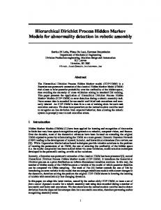
Fig 3. Performance comparison of HCC with diagonal models with increasing number of mixtures In Figure 3, we first show the recognition performance (in WER) of several diagonal model sets as a function of their mixture numbers in each tied-state. We increase the mixture number from 6 in the baseline model set up to 12. When the number of mixture components reaches 8 (the error rate is 4.00%), the word error rate reduction compared with the baseline is only 1.96%. This shows that it can not significantly improve the performance over our baseline model by simply increasing the number of diagonal Gaussian mixtures. We also plot the HCC’s performance in the figure as an isolated diamond point. From the results, it is clear that the HCC yields much better performance than the diagonal model set with even larger number of mixtures. 6.

EXPERIMENTS (II): CHINESE DICTATION TASK

In this section, the above HCC method is evaluated in a larger database, i.e., an in-house Chinese dictation task. The baseline system is the MSRA Mandarin Speech Toolbox [12]. We added more training data to the toolbox. A total of 49378 sentences from 250 speakers (totally 75 hours) are used for training. The baseline model set is a CDHMM set with 16 mixtures of Gaussian components with diagonal covariance matrices for each tied state. A total of 500 sentences from 25 speakers are used for word-loop decoding in the level of Chinese characters. The tied-state number is 5114. The error rate of Chinese character of the baseline system is 21.14%, while that of HCC with decision tree is 18.07%. We got 14.52% error rate reduction.

I - 676

[1] A. Ljolje, “The importance of cepstral parameter correlation in speech recognition”, Comput. Speech Lang., vol. 8, pp. 223~232, 1994. [2] S. B. Davis and P. Mermelstein, “Comparison of parametric representations for monosyllabic word recognition in continuously spoken sentences,” IEEE Trans. Acoust., Speech, Signal Processing, vol. 28, pp. 357, 1980. [3] Haeb-Umbach, R. and Ney, H., “Linear discriminant analysis for improved large vocabulary continuous speech recognition”, in Proc. ICASSP’92. [4] R. A. Gopinath. “Maximum likelihood modeling with Gaussian distributions for classification”. in Proc. ICASSP’98. [5] N. Kumar, “Investigation of silicon-auditory models and generalization of linear discriminant analysis for improved speech recognition,” Ph.D. dissertation, Johns Hopkins Univ., Baltimore, MD, 1997. [6] M. J. F. Gales, “Semi-tied covariance matrices for hidden Markov models”, IEEE Trans. Speech Audio Processing, vol. 7, pp. 272–281, 1999. [7] M. J. F. Gales, “Maximum Likelihood Multiple Subspace Projections for Hidden Markov Models”, IEEE Trans. Speech Audio Processing, vol. 10, pp. 37–47, 2002. [8] Vanhoucke, V. and Sankar, A. “Mixtures of inverse covariance”, IEEE Trans. Speech Audio Processing, vol. 12 , pp. 250 - 264, May 2004 [9] S. Axelrod, R. Gopinath, and P. Olsen, “Modeling with a subspace constraint on inverse Covariance matrices”, in Proc. ICSLP 2002. [10] Olsen, P.A.; Gopinath, R.A., “Modeling inverse covariance matrices by basis expansion”, IEEE Trans. Speech and Audio Processing, vol. 12, pp.37 - 46, Jan. 2004 [11] Shinoda, K. and Lee, C.-H., “A structural Bayes approach to speaker adaptation”, IEEE Trans. Speech and Audio Processing, vol. 9, pp:276 - 287, March 2001 [12] E. Chang, Y. Shi, J. Zhou, and C. Huang, “Speech lab in a box: A Mandarin speech toolbox to jumpstart speech related research toolbox,” in Proc. Eurospeech 2001