The hierarchical edge bundle method clusters the graph edges to better understand ... the same part of the control structure are drawn near each other to form ...
Hierarchical Edge Bundles for General Graphs Yuntao Jia, Michael Garland and John C. Hart
Technical Report
June 2009
Abstract The hierarchical edge bundle method clusters the graph edges to better understand and analyze graphs, but its effectiveness relies critically on the quality of the hierarchical organization of its nodes and edges. This paper proposes a novel graph visualization approach that extracts the community structure of a network and organizes it into a more balanced and meaningful hierarchy so that its edge bundle rendering better indicates its structure. Results on several data sets demonstrate that this approach clarifies realworld communication, collaboration and competition network structure and reveals information missed in previous visualizations.
1
Introduction
Graph visualization is becoming a crucial tool for understanding and analysis of an ever expanding collection of social communication and collaboration networks. As such networks and the connections they represent become larger and more complex, traditional straight-line graph drawings become less effective at revealing structure, which has lead to the development of many new visualization techniques, including e.g. graph clustering, graph filtering and edge bundles. Among these recent approaches, edge bundles is particularly effective at depicting communication in a network by depicting edges as curves and collecting them to reveal an underlying graph “control” structure. Since the control structure is often much simpler than the graph itself, edge curves representing the same part of the control structure are drawn near each other to form bundles which drastically remove the visual clutter of edge crossings. This has the benefit of more clearly depicting a larger graph’s structure, but relies on the availability and quality of additional information needed to properly bundle the edges into a coherent control structure which limits their application. For example, the hierarchical edge bundle method [15] needs a pre-defined hierarchy, and geometry-based edge clustering [7] needs geometric positioning information. We propose a new approach that automatically builds hierarchical edge bundles for general graphs without requiring any extra information. Based on the motivation in Sec. 3, we first find well-connected nodes within small communities and place them at the base of the hierarchy. We then progressively merge these communities based on their affinity to form the upper levels of the organizational hierarchy. We can automatically construct a community hierarchy following Girvan and Newman [12]. First graph edges are filtered to remove all but those with the lowest betweenness centrality. The remaining edges connect nodes in relatively small communities. Smaller communities are merged into larger communities if they are connected by edges, and the merging order is determined by the betweenness centrality of these community connecting edges. Such repeated merging in increasing BC-order yields a “dendrogram” whose organizational hierarchy can be severely imbalanced to look more like a collection of lists than a balanced tree hierarchy. To better prepare this structure for use in organizing a hierarchical edge bundle visualization, we balance the tree and reduce its overall depth. As tested on various graphs, the approach is very efficient and yields both meaningful graph community hierarchies as well as effective and pleasing edge bundle visualizations. An additional novel contribution of this community hierarchy is the ability to measure the relative strength of the communities. The choice of which communities to merge is sometimes obvious and sometimes arbitrary, based on the distribution of the betweenness centrality of edges between communities. We quantify the obviousness of this merging choice, call it the “BC differential,” use it to indicate the strength of the community and depict this strength as bundle tension in the hierarchical edge bundle visualization. The rest of the paper is organized as follows. Sec. 2 reviews related work on edge bundles, clustering nodes and edges into hierarchies and computing betweenness centrality. Sec. 3 discerns, through comparisons and discussion, the kind of hierarchies that work best for hierarchical edge bundle visualization, leading to the algorithm described in Sec. 4. The results in Sec. 5 show that this approach greatly improves the visualization of networks by clustering communication into meaningful hierarchies of topics, and discusses user interaction and analyzes its accuracy vs. speed tradeoffs. Sec. 6 concludes with ideas for future work on larger graphs and time-varying networks.
1
Managing Director Director Traders Lawyer Manager
Vice President President
Employee
CEO
N/A
Manual (ideal)
Small Worlds [1]
Strict BC [12]
Balanced BC (this paper)
Figure 1: Comparison between different hierarchies (top) and their hierarchical edge bundles (bottom) on graph “enron-email-2001.08.”
2
Previous Work
Our approach builds on and extends hierarchical edge bundles by automatically building a control hierarchy using an approach that extends the poor hierarchy generated by Girvan and Newman’s betweenness centrality community filter. This section reviews the previous work in each of these areas. Edge bundles render large graphs via edge clustering, by collecting together long edges analogous to the way electric wires are merged into bundles along a shared mutual path segment, fanning out at ends to connect distinct endpoints. Holten [15] proposed hierarchical edge bundles to visualize a compound graph accompanied by a predefined hierarchy. His approach first drew the hierarchy using an existing tree layout method, such as a radial layout [9]. It then laid out long and complex graph edges using the nodes of the tree as B-spline control points. Each edge in the original graph was modeled as a single B-spline using the control points along the shortest path in the hierarchy from one end node to the other in the hierarchy. Cui et al [7] visualized large graphs via edge clustering through a geographical control structure. Balzer and Deussen [4] used edge bundles to simplify edges in a clustered level-ofdetail graph visualization, that filtered the layout of the original graph. Confluent drawing [8] displayed non-planar node-link diagrams using curved edges, though not all graphs are confluently drawable. Flow map layouts [20] route edges through a binary cluster hierarchy, though only for single-source graphs. Our approach relies on hierarchical edge bundles, but generates a control hierarchy automatically for any input graph. Graph hierarchies are often created by repeated graph clustering, where nodes are clustered to indicate node affinity groups. Herman et al. [14] summarizes a number of these methods and their application to visualization. More recently, Wu et al. [23] hierarchically clustered nodes by their shortestpath distance from hub nodes (chosen by least betweenness centrality or highest degree) for data mining and visualizing power-law graphs. Kumar and Garland [17] clustered nodes based on an authority metric and stratified the graph into different layers for faster layout and overlaid for interactive visualization. Graph hierarchies can also be created by filtering. Auber et al. [1] filtered out weak edges in a “smallworld” graph to generate and visualize a hierarchy of strongly connected components. Chiricota et al. [6] applied similar ideas based on edge strength to discover components structure in software systems. Betweenness centrality (BC) measures how often an edge is on the communication paths among all other nodes. High-BC edges connect large communities, whereas low-BC edges connect individuals within a community. Girvan and Newman [12] removed high BC edges to reveal community structures in
2
social and biology networks, and this approach was later surveyed and compared with other approaches by Newman [19]. Heer and Boyd [13] removed high-BC edges to reveal communities within social networks, whereas Jia et al. [16] removed low-BC edges to reveal the communication pathways within social networks. We combine these approaches, using low-BC edges to detect and cluster communities, and simplifying high-BC edges to accentuate the communication pathways between communities.
3
Motivation
Our approach extends the hierarchical edge bundle (HEB) graph rendering method, which requires a pre-defined control hierarchy for general graphs, by automatically constructing a community hierarchy. A community hierarchy is a tree structure whose leaves represent graph nodes and parents represent affinities that collect graph nodes into communities. These affinities are hierarchical so communities can contain sub-communities, but communities are otherwise mutually exclusive. Unless one community is the direct ancestor of another, a graph node could not belong to both communities. Hence they are good for hierarchies of exclusive labels or segmentations, but not appropriate e.g. for multiple attribute or tag categorization. We construct a community hierarchy by repeated cluster merging. Given some (yet undefined) community affinity metric, we first decompose the graph into many small tight-knit communities of a few nodes of which the dense interconnections maximize the affinity metric. We then merge smaller tighter-knit communities into larger, looser communities in order of decreasing affinity metric measured between communities. Repeated merging yields a community hierarchy and concludes with its root representing the community of all nodes in the original graph. We use this community hierarchy to control the layout of both graph nodes and graph edges. We place all of the graph nodes on the perimeter of a circle or other polygon. The graph nodes are placed in the sequence of an in-order traversal through the community hierarchy to cluster their position on the perimeter according to community. We then use a radial tree layout [9] to place the parent tree nodes of the community hierarchy in the interior region of the surrounding perimeter leaf nodes. In addition to the nodes, the layout of graph edges in this representation is also managed by the community hierarchy by using it to control hierarchical edge bundling. HEB depicts an edge between graph nodes as a B-spline curve whose control points are the hierarchy node radial-layout positions along the shortest tree path between the two leaf nodes in the hierarchy corresponding to the two graph nodes. For common graphs, such as those that represent social networks, there are more edges within a community than between communities. The within-community nodes are proximate due to the hierarchy’s radial layout which localizes their dense edge layout, whereas the fewer edges between communities should follow different shortest paths through the hierarchy to avoid collision and remain discernable through the interior region of the radial layout. Fig. 1 illustrates the motivation of our approach by demonstrating the results of hierarchical edge bundle visualization of the email network between former Enron employees in August 2001. Individual email communications are represented as B-spline curved edges from senders (red) to receivers (green). The effectiveness of the HEB visualization relies on the quality of the community hierarchy. The manual example, based on the Ex-Enron employee status report [21], serves as ground truth for the semantics of the community hierarchy, though its shallow depth creates a mish-mash of edges in the interior and large fanouts to the nodes. Automatic community hierarchy methods can be problematic. For example “small worlds” [1] does not detect these communities as well. The betweenness centrality metric does find such communities, but the hierarchy generated by Girvan and Newman [12] is significantly imbalanced, yielding lists instead of hierarchies. Balancing the hierarchy generated by betweenness centrality yields a much better organization and layout, that is more amendable to the advantages of hierarchical edge bundle visualization. Balanced community hierarchies better facilitate user perception for two reasons. First, the depth is greater in an unbalanced tree, which further complicates the visual task of following a single edge from one peripheral node to another. Second, imbalance concentrates more edges through the root and ancestry of a hierarchy, which makes thicker edge bundles that are harder to follow. Tree rotations can balance a lopsided tree [3], but rotation changes the hierarchical organization of a tree which would change the community structure of the underlying graph. The next section describes a better approach that re-defines the merging rules that create the community hierarchy to yield a more 3
balanced tree while retaining the fidelity of Girvan and Newman’s BC-based communities.
4
Balanced Community Hierarchy Construction
We construct a balanced community hierarchy for an input graph in three steps, illustrated in Fig. 2. We first compute the betweenness centrality of every edge in the graph, and remove edges in non-increasing order of BC to find the smallest communities that collectively form the base of the hierarchy. We then construct the hierarchy by merging these communities according to the increasing BC of the removed edges. Third, we adjust the newly created hierarchy to facilitate its radial layout. This yields a completed hierarchy to enable the hierarchical edge bundle visualization of the original graph. a
c
a
c
b
d
b
d
a
Input graph
c
b
c
b
d
d a
Filter edges
a
Create subtrees
b
c
d
Merge to a single hierarchy
Hierarchical edge bundles
Figure 2: Work flow of our approach.
4.1
BC Edge Filtering
Betweenness centrality [10] indicates how often a node lies on the shortest and presumably most used communication paths between other nodes X σu,w (v)/σu,w BC(v) = (1) u6=v6=w∈V
where σu,w counts the number of shortest paths between u and w, and σu,w (v) counts only the ones containing v. High BC edges typically connect communities of nodes within which connections are dense but between which connections are loose [12]. The bigger the BC, the larger the communities. In contrast, low BC edges usually connect nodes within the same community. In particular, an edge BC of 1 (the smallest allowed) indicates it connects two nodes clearly in the same community, and these two nodes form the smallest possible community. Girvan and Newman [12] detect communities in a graph by removing edges in descending BC order, which leaves small disjoint communities of nodes connected by the remaining edges. We augment their process with the additional rules: • an edge < a, b > is removed only if min(deg(a),deg(b)) ≥ 2, and • an edge e is removed only if BC(e) > 1. The first rule ensures that every node retains its least BC edge, and the second establishes a target termination condition where every remaining edge has unit BC. We also place removed edges on a stack so we can reintroduce them in LIFO (last-in-first-out) order.
4.2
Merging Communities
The numerous small communities that result from edge filtering are detected by a simple connected component sweep. We convert these small components into a forest of small subtrees to form the bottom of the hierarchy, illustrated in the third step of Figure 2. We then merge subtrees according to the previously removed edges in order of increasing BC. If a removed edge connected a pair of nodes from two subtrees, then those two subtrees belong to a bigger community in the original graph. Since the filter pushed removed edges onto a stack in descending order of BC, popping these edges from a stack produces increasing BC edges that merge communities in the correct order. 4
Ta
Sa
Tb
e < a, b >
na nb
na nb
Figure 3: Merging two community hierarchies. Here two communities are connected because a node in Ta is connected by an edge to a node in Tb . Merging two subtrees can lead to imbalance unless certain rules are followed. If a removed edge < a, b > connects two graph nodes a and b belonging to two different communities represented by the current subtrees Ta and Tb , then Ta and Tb are merged based on the two following rules. • If height(Ta ) = height(Tb ), then a new node is added as parent of both Ta and Tb . • If height(Ta ) > height(Tb ), then we find the subtree Sa ⊂ Ta whose community includes a such that height(Sa ) = height(Tb ) and add Tb as a child of the parent of Sa . The second rule is illustrated in Fig. 3. It ensures that merging trees of different height does not increase the height of the result by more than one. This differs significantly from Girvan and Newman [12] where every merge increases the height of the result. In fact the approach of Girvan and Newman yields a tree of worst-case O(n) height for n nodes. The worst case height under our rules is O(log n) by induction. If we have two nodes, the height is one and the claim is satisfied. If we have a subtree of height k then by assuming the proposition it has O(2k ) nodes, then under the second rule, we would not increase its height unless we had another tree of at least that height. Even if we did, the merged tree would then have height k + 1 and consist of O(2k+1 ) nodes. These new merging rules make more sense for both community detection and hierarchical edge bundle visualization. For community detection, a reintroduced graph edge < a, b > defines a larger community by connecting two communities that contain a and b. However, node a may belong to several communities, represented as nested subsets by an ancestry path in the community hierarchy. We must select one of these communities of a to merge with the community of b, so we merge the largest communities of both that share the same level in the hierarchy with the assumption that they represent the same kind of community. While this assumption is often incorrect, Girvan and Newman [12] often merge a very small community with a very large community, leading to rather jagged and lopsided hierarchies as shown in Fig. 1. For hierarchical edge bundles, a Girvan-Newman hierarchy routes communication from one community to another through a shared parent (the current root during the tree merging process). Sending all communications that far up and then back down unnecessarily increases the edge density in the interior of the radial layout of the HEB, as shown in Fig. 1. Merging subtrees at the minimum height yields simpler and shorter communication pathways in the HEB, leaving the interior to represent and highlight more significant cross-community communication.
4.3
Adjusting the Hierarchy
We use radial layout [9] to position the nodes of the community hierarchy. Such layouts work best for trees of uniform depth, otherwise multiple radii are needed as demonstrated in Fig. 1. Though our community hierarchy construction rules strive for uniform depth they do not always achieve it. Furthermore, the chosen root of the tree might not represent the mass center of the graph nodes at its leaves. In severe cases, this can lead to a biased drawing as shown in Fig. 4. To better prepare the community hierarchy for radial layout, we apply a few simple adjustments. First we explore different root node choices to recenter the radial tree layout so that no child of the root node represents more than half of the original graph nodes. (This is feasible if the root has more than 5
Original Graph
Extracted Hierarchy
Fixed Root
Kenneth Lay
Fixed Depth
Edge Bundles
Selected visualization
Figure 4: Construction of balanced community hierarchies for graph “enron-email-2001.08.” two children.) If a root’s child is found to represent more than half the nodes, then we set it to be the new root and automatically retest the hierarchy, as shown in Fig. 4. We also strive to have all of the leaves of the hierarchy at the same level. If through a bottom-up search we find a node whose children represent different heights, we insert dummy nodes to make their heights equal.
4.4
Measuring Community Strength
We detect communities based on edge betweenness centrality and low BC edges connect nodes in small communities. The BC of intra-community edges is lower than that of inter-community edges. A community is strong if this margin is large. In other words, we can measure the strength of a community by measuring the BC difference between intra-community edges and inter-community edges. We call this the “BC differential” and we use it to indicate for each community hierarchy node whether the choice of which two communities to merge was obvious or arbitrary. To be more precise, for each community hierarchy node, we define intra-community edges to be the edges connecting that hierarchy node’s children to each other, which means this node is the lowest common ancestor (LCA) in the shortest path between its child communities. For inter-community edges, we count the edges that connect leaves from the node’s community to its sibling communities, which means the node’s parent is the LCA of the shortest path between the leaves. Besides measuring the strength of communities, we use the BC differential to control the HEB drawing. In particular, we set the edge bundle B-spline tension proportional to the BC difference. A node with high BC difference represents a strong community and we increase the tension of B-splines through that control point to make the edge bundles more compact near that node.
6
IA Independents Mid-American Big East Big Ten Atlantic Coast Conference USA Southeastern Pacific-10 Mountain West Big 12 Big West Western Athletic
Figure 5: Graph ”college-football-2000” visualized with edge bundles. First row: Original graph, original graph with hierarchical edge bundles. Second row: hierarchy created with Girvan and Newman’s approach [12] and hierarchy created with our method.
5
Results and Discussion
We have tested our algorithm with several real data sets to demonstrate its effectiveness in both visualization and community detection. In all the results, we use the GEM method [11] to layout the original graph. Based on whether the graph is directional or not, we have applied different color mappings in their hierarchical edge bundle visualizations. For directed graphs, we color source nodes with red and target nodes with green. For undirected graphs, we color nodes in a hue color mapping based on their polar angles in the radial layout. In both cases, the color is linearly interpolated along the B-spline that is used to visualize the edge. Figure 5 visualizes the undirected graph “college-football-2000”1 which represents 616 matches between 115 Division IA college football teams during regular season fall 2000 [12]. What makes this data set interesting is that its community structure is known. In particular, those teams belong to 11 conferences except a few independent teams that do not belong to any conference. Games were played more frequently between teams in the same conference. Like Girvan and Newman’s [12], the hierarchy constructed by our approach discovers these conference communities and clusters teams in the same conference as siblings to each other. The independent teams are placed in conferences they played more with. This confirms that our method correctly detected the communities within this graph. Girvan and 1 Available
at URL http://www-personal.umich.edu/˜mejn/netdata/
7
Newman [12] also captured the team conferences, but their unbalanced hierarchy does not fit well with the hierarchial edge bundle visualization. Figure 4 visualizes the directed graph ”enron-email-2001.08”, which represents the 389 emails between 132 Enron employees in August 2001, extracted from cleaned Enron email data [22]. Red represents senders and green represents recipients. We only considered the ”TO” recipients and ignored the ”CC” or ”BCC” recipients. The graph can be visualized more effective with the hierarchy constructed by our method. In that month, Kenneth Lay is named the CEO of Enron, and by interactively selecting his node, we can see a lot of emails from him to all other employees in various communities including his own. We also found partial ground truth organization structure from the SocialRank project [18], shown in Fig. 6. Our method discovers similar results. The relevant employees are user labeled and emails between them are also visualized by user selection.
Mark Tylor Mark Haedicke Kay Mann Elizabeth Sager Christian Yoder
Stacey White Susan Bailey Sara Shackleton Stephanie Panus Tana Jones Williams Jason Marie Heard
Figure 6: The organization ground truth (top) of Enron employees during Jan. 2000 and Nov. 2001. Similar results (bottom) discovered with our community hierarchy detection method. Figure 7 visualizes the undirected graph ”myfacebook” which represents the network between 165 facebook friends of the first author. By the nature of social networks, the graph is highly connected with 1803 edges. The generated hierarchy detects different groups of my friends, including friends in the same department which further includes my lab mates, friends from my previous college, senior colleges who have spent more years here than me, junior colleges who have spent less years here than me, friends from a registered student organization (RSO) that I worked with, friends that I played soccer with, and friends in a summer internship program. The hierarchical edge bundle visualization is also shown and leads to some discovery. First, my internship friends do not know my other friends because they are from different colleges. There are a few exceptions for interns from the same college as me. Second, there are many connections between my current department friends and friends from my previous college. This is simply because after graduation 8
they joined the same college and same department as me. Figure 8 visualizes the undirected graph “sp500-38,” which represents 3206 cross correlations of price fluctuation of 365 stocks from the S&P 500. Our method is able to recognize different stock sectors and put them near to each other in the hierarchy. The hierarchical edge bundles visualization reveals that financial stocks affect all other kind of stocks except energy, consumer staples and health stocks, which are relatively independent. The proposed method is very efficient. Most operations have linear complexity with two exceptions. One is betweenness centrality which can be computed in O(nm) time for unweighted graphs and O(nm+ n2 log n) time for weighted graphs [5], where n and m are the numbers of nodes and edges respectively. The other is sorting edges in descending order of BC before removing edges, which requires running time of m log(m). All presented results can be computed within seconds for the graphs shown.
5.1
Quality of the Communities
Figure 9 shows the BC-differential measured on the graph “college-football-2000” and visualized on the hierarchy with pseudo color mapping. Nodes with high BC difference indicate strong communities, which coincide with the conferences of those teams. Smaller BC difference nodes indicate weaker, somewhat arbitrary, choices for communities because their intra-community edges and inter-community edges have smaller difference in BC. The middle image in Figure 9 demonstrates the rendering of the BC-differential metric for community strength, depicted by the tension of B-spline control points in the hierarchical edge bundle. We marked two nodes with dashed rectangles. One of them has much higher BC difference than the other and its edge bundles are more compact in the visualization to illustrate that it is a strong community. We further use this information to discover more accurate community information from the graph. In particular, we remove nodes in the hierarchy if their BC differences are lower than a threshold. The result is shown in the right image of Figure 9 with a threshold of ten. Only strong communities are preserved here and they are more close to the conferences of those teams.
5.2
Accuracy v. Speed
Users also have control over the tradeoff between accuracy and speed in our algorithm. In particular, when removing edges, we only compute the BC once to determine the order of all edges, which saves computation time. If accuracy is more important, then BC can be recomputed after removing each edge, as done in the approach by Girvan and Newman [12]. For ”college-football-2000,” the static BC case, the Big 12 and Big West conferences are merged into a bigger community, as shown in the first image in Figure 11. By recomputing a dynamic BC after each edge is removed during the filtering process, those two conferences end up well separated, as shown in the first image in Figure 10. The hierarchy is more accurate and similar to the community ground truth, which is shown in the second image. We oriented the latter for better comparison. However this incurs the additional time complexity of a factor of m in each edge removal step.
5.3
User Interactions
We have implemented our algorithm in a visualization tool which also supports several simple but effective user interactions. First, users can modify the hierarchy based on their knowledge or other extra knowledge about the data. Two operations are provided: moving and swapping. The moving operation allows users to change the parent of a chosen node. The swapping operation allows users to swap two hierarchy nodes with each other. In both cases, the same operations affects the descendants of the selected node(s). An example on the graph ”college-football-2000” is shown in Figure 11. In the hierarchy constructed by our method, several teams from Big 12 and Big West conferences were mixed together. The visualization is shown in the left image. The user moved several involved Big 12 teams to separate those two conferences. The visualization after the interactions is shown in the right image. Users can also filter displayed edge bundles by selecting or deselecting graph nodes. For the graph “college-football-2000,” the user can perform queries such as “display only the Illinois’ games.” The results are shown in the left image in Figure 12. Users can also select a community of nodes by selecting the corresponding parent node in the community hierarchy. 9
Our tool also takes advantage of the HEB visualization. For example, users can change the strength of the edge bundles to change the bundle compactness. An example on the ”college-football-2000” is shown in the right image of Figure 12 where the strength is changed to 0.65. Users can also change the edge bundle transparency or apply different color mappings.
6
Conclusion and Future Work
We modified Girvan and Newman’s [12] BC-based community detector into a more balanced community hierarchy which we showed works significantly better for HEB graph visualization, allowing HEB to be applied to a wider variety of graphs without the need of an associated pre-defined hierarchy. We also implemented this method as part of an interactive graph visualization tool, where the user can modify and manipulate the visualization for knowledge discoveries. We also discussed methods to assess the quality of the discovered hierarchies, further facilitating users to understand the community structure residing in graphs. One future direction for this approach is extending it to larger graphs. One concern is the radial layout used to draw the hierarchy. When there are too many nodes, drawing them on a single circle spaced nodes too closely, and the B-spline curve paths representing edges become unusable. Another scalability concern is the superlinear computation time of betweenness centrality, which can be addressed through approximation [2]. Another idea is to extend this approach to time-varying or even real time data, such as real time messages or email within a social network. How to extract a hierarchy that is meaningful over time and how to update the hierarchy smoothly will be the key issues to solve.
References [1] D. . Auber, Y. Chiricota, F. Jourdan, and G. Melancon. Multiscale visualization of small world networks. In INFOVIS ’03: Proceedings of the IEEE Symposium on Information Visualization (INFOVIS’03), pages 75–81, 2003. [2] D. A. Bader, S. Kintali, K. Madduri, and M. Mihail. Approximating Betweenness Centrality, pages 124–137. Springer, 2007. [3] J.-L. Baer and B. Schwab. A comparison of tree-balancing algorithms. Commun. ACM, 20(5):322– 330, 1977. [4] M. Balzer and O. Deussen. Level-of-detail visualization of clustered graph layouts. Asia-Pacific Symposium on Visualization, 0:133–140, 2007. [5] U. Brandes. A faster algorithm for betweenness centrality. J. Math. Soc., 25(2):163–177, 2001. [6] Y. Chiricota, F. Jourdan, and G. Melancon. Software components capture using graph clustering. In Program Comprehension, 2003. 11th IEEE International Workshop on, pages 217–226, 2003. [7] W. Cui, H. Zhou, H. Qu, P. C. Wong, and X. Li. Geometry-based edge clustering for graph visualization. IEEE Transactions on Visualization and Computer Graphics, 14(6):1277–1284, 2008. [8] M. T. Dickerson, D. Eppstein, M. T. Goodrich, and J. Y. Meng. Confluent drawings: visualizing non-planar diagrams in a planar way. In Proc. 11th Int. Symp. Graph Drawing (GD 2003), number 2912 in Lecture Notes in Computer Science, pages 1–12. Springer-Verlag, September 2003. [9] P. Eades. Drawing free trees. Bulletin of the Institute for Combinatorics and its Applications, 5:10–36, 1992. [10] L. C. Freeman. A set of measures of centrality based upon betweenness. Sociometry, 40(1):35–41, 1977. [11] A. Frick, A. Ludwig, and H. Mehldau. A fast adaptive layout algorithm for undirected graphs. In GD ’94: Proceedings of the DIMACS International Workshop on Graph Drawing, number 894, pages 388–403, 1994. 10
[12] M. Girvan and M. E. Newman. Community structure in social and biological networks. Proc Natl Acad Sci U S A, 99(12):7821–7826, June 2002. [13] J. Heer and D. Boyd. Vizster: Visualizing online social networks. In INFOVIS ’05: Proceedings of the Proceedings of the 2005 IEEE Symposium on Information Visualization, page 5, 2005. [14] I. Herman, G. Melan¸con, and M. S. Marshall. Graph visualization and navigation in information visualization: A survey. IEEE Transactions on Visualization and Computer Graphics, 6(1):24–43, 2000. [15] D. Holten. Hierarchical edge bundles: Visualization of adjacency relations in hierarchical data. Transactions on Visualization and Computer Graphics, 12(5):741–748, 2006. [16] Y. Jia, J. Hoberock, M. Garland, and J. Hart. On the visualization of social and other scale-free networks. IEEE Transactions on Visualization and Computer Graphics, 14(6):1285–1292, 2008. [17] G. Kumar and M. Garland. Visual exploration of complex time-varying graphs. IEEE Transactions on Visualization and Computer Graphics, 12(5):805–812, 2006. [18] J. Montemayor, C. Diehl, M. Pekala, and D. Patrone. Socialrank: An ego- and time-centric workflow for relationship identification. In HCIR2008. Microsoft Research, 2008. [19] M. Newman. Detecting community structure in networks. The European Physical Journal B Condensed Matter, 38(2):321–330, March 2004. [20] D. Phan, L. Xiao, R. Yeh, P. Hanrahan, and T. Winograd. Flow map layout. In INFOVIS ’05: Proceedings of the Proceedings of the 2005 IEEE Symposium on Information Visualization, pages 219–224, 2005. [21] J. Shetty and J. Adibi. The Enron email dataset database schema and brief statistical report. Information Sciences Institute Technical Report, University of Southern California, 2004. [22] J. Shetty and J. Adibi. Discovering important nodes through graph entropy the case of enron email database. In LinkKDD ’05: Proceedings of the 3rd international workshop on Link discovery, pages 74–81, 2005. [23] A. Y. Wu, M. Garland, and J. Han. Mining scale-free networks using geodesic clustering. In KDD ’04: Proceedings of the tenth ACM SIGKDD international conference on Knowledge discovery and data mining, pages 719–724, 2004.
11
Original graph
Edge Bundles
My dept. friends My lab mates Friends from prev. college Senior colleges Junior colleges RSO friends Soccer friends Internship friends
Generated Hierarchy (with user supplied labels) Figure 7: Graph ”myfacebook,” including user supplied labels of communities discovered by our automatic hierarchy generation method.
12
Original graph
Edge Bundles
Fianancials Health Care Information Technology Energy Consumer Staples Material Industrials Consumer Discretionary
Generated Hierarchy (with user supplied labels) Figure 8: Graph ”S&P500” including user supplied labels of communities discovered by our automatic hierarchy generation method.
13
Big Ten Big East
Atlantic Coast Conference USA
Mid-American
Western Athletics
Southeastern Big 12 & Big West
Pacific-10 & Mountain West
Figure 9: Measuring quality of communities with BC differentials on graph ”college-football-2000.”
Big West
Western Athletics
Big West
Western Athletics Mountain West
Big 12
Mountain West Big 12 Big East
Big East Pacific-10
Pacific-10 Atlantic Coast
Atlantic Coast SoutheasternEastern DIV
Mid-American
Mid-American Southeastern
Big Ten
SoutheasternWestern DIV IA Indepdents Conference USA
IA Indepdents
Big Ten
Conference USA
Figure 10: Community hierarchy constructed with recomputing BC compared to the community ground truth of graph ”college-football-2000.”
Figure 11: A user interactively modify the community hierarchy of graph ”college-football-2000” to separate two conferences.
14
Illinois
Middle Tennessee State California San Diego State
Figure 12: Manipulating a hierarchical edge bundle visualization on graph ”college-football-2000”.
15