Visualizing Edge-Edge Relations in Graphs - CiteSeerX

Visualizing Edge-Edge Relations in Graphs Corinna Vehlow∗ , Jan Hasenauer† , Fabian J. Theis† , and Daniel Weiskopf∗ ∗ †

VISUS – Visualization Research Center, University of Stuttgart, Germany

Institute of Bioinformatics and Systems Biology, Helmholtz Center Munich, Munich, Germany

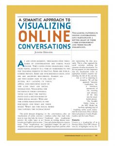
Figure 1: Financial transaction data of 249 transactions between 181 accounts visualized as directed straight links connecting vertices and hence representing relations between objects. The blue curves represent edge-edge relations, thereby connecting pairs of transactions that vary in amount drastically, although assigned the same set of keywords. Left: Loops attached to transactions represent temporal patterns (emphasized by the green arrows), i.e., reoccurring transactions of diverging amounts between the same accounts. Right: Selection of four transactions whose amounts vary from many other transactions that have the same keywords.

A BSTRACT Graphs are used to model relations between sets of objects. Objects are represented by vertices and relations by edges of the graph. Besides vertex-vertex relations, in some application domains also relations between edges exist. Our new visualization approach supports the investigation of both relation types in one diagram. Edge-edge relations are visualized as curves that are directly integrated into the node-link diagram that represents the object-relation structure. In contrast, vertex-vertex relations are illustrated distinguishably from edge-edge relations using straight links as representations. While the shape of links is used to differentiate between the relation types, the weights of the edge-edge relations are mapped to the width and color of the curves. To facilitate an extensive analysis of interrelations, our approach incorporates several interaction techniques that can be used for filtering and highlighting. The usability of our visualization is demonstrated with two case studies in the application domains of bioinformatics and financial services. Keywords: Graph visualization, correlation visualization, multivariate graph data. Index Terms: H.5.2 [Information Interfaces and Presentation]: User Interfaces—Graphical user interfaces (GUI); E.1 [Data]: Data Structures—Graphs and Networks; J.3 [Computer Applications]: Life and Medical Sciences—Biology and genetics; 1 I NTRODUCTION Graphs are a common way to describe relations between objects, where both objects and relations are oftentimes multivariate. For re∗ E-mail: † E-mail:

{vehlow,weiskopf}@visus.uni-stuttgart.de {jan.hasenauer,fabian.theis}@helmholtz-muenchen.de

IEEE Pacific Visualisation Symposium 2013 26 February - 1 March, Sydney, NSW, Australia 978-1-4673-4799-0/13/$31.00 ©2013 IEEE

lations, such multivariate data might describe a time series of edge weights or in general a vector of properties describing the vertexvertex relations (VVRs). These multivariate VVRs might be interrelated among each other. Such edge-edge relations (EERs) can be derived implicitly based on correlation or similarity measures for the respective multivariate attribute vectors. Of course, EERs could also be independent from properties of VVRs, if they are given explicitly in the data model. For biochemical reaction networks (BRNs) [23], EERs exist for reaction parameters or fluxes. Interdependencies between reactions can occur, e.g., if one reaction influences the concentration of the substrate of an other reaction. Furthermore, EERs can be used to describe correlations between samples of potential parameters inferred from experimental data. The analysis of correlations between these samples is essential to assess the uncertainty of the simulated attributes. Other possible applications include dynamic weighted social contact or citation networks, within that the change of the weight of a particular edge might be correlated or anti-correlated with the change of weight of another edge. Anti-correlations in a social contact network, e.g., would demonstrate that an increasing amount of contact to some people, directly comes along with less contact to others. The most prominent visual metaphor to encode relational data is the node-link diagram [7, 11]. Besides node-link diagrams, visual adjacency matrices are popular representations of relational data. With these existing techniques, VVRs and weighted EERs could be visualized using two separate views (see Figure 2): for example, a node-link diagram representing VVRs and an additional node-link diagram representing EERs. The similarity or correlation measures between VVRs could thereby be mapped to the color of links within the additional view (see Figure 2(b)). The use of two views calls for the use of brushing and linking to allocate elements, e.g., to highlight the respective two VVRs the selected EER connects. However, already the selection of several EERs would pose a problem, as a consistent highlighting of the respective links (VVRs) would

201

(a) Highlighted VVRs (thick links): A154→A64, A175→A19, A175→A34, and A175→A50

(b) Highlighted EERs (curved links): A154→A64 ⇔ A175→A19, A154→A64 ⇔ A175→A34, and A154→A64 ⇔ A175→A50

Figure 2: Visualization of VVRs and EERs of the graph from Figure 1 using separate linked views. (a) Node-link diagram of directed VVRs using clockwise curved links; each VVR is assigned a different color (hue). (b) Node-link diagram of EERs; nodes represent VVRs of (a) and are therefore colored in the same fashion. The strength of dissimilarity is mapped to the color and width of the links.

not be bijective without the use of labels. Furthermore, when visualizing EERs out of context, i.e., separate from the graph structure, it is hard to extract circular dependencies between VVRs or dependencies between relations within a subnetwork or community of the graph. Hence, the use of two views impedes path-oriented tasks. These become even harder using an adjacency matrix instead of a node-link representation to visualize EERs. To support an investigation of the structural context of related VVRs, we suggest visualizing EERs directly in the context of the node-link diagram showing relations between objects. To the best of our knowledge, there exists no such visualization approach for EERs. Our visualization approach uses two different edge representations within node-link diagrams that facilitate an easy differentiation between VVRs and EERs. While the shape of the links is used to indicate the type of relation, the visual attributes color and width are used to visualize the weights of EERs. The usefulness of our visualization technique is illustrated by two case studies analyzing (anti-)correlations between parameter and flux samples in biochemical reaction networks and (dis-)similarities of financial transactions between a set of accounts. 2 R ELATED W ORK As mentioned before, node-link diagrams are a commonly used representation for graphs. They are intuitive and effective for perceiving relations between objects and for solving path-related tasks, as they exploit Gestalt principles [24] of closure and good continuation. When using node-link diagrams, vertices are mapped to geometric forms such as circles or squares and relations among them are expressed by straight or curved links. Depending on the application domain, these relations can be used to describe interactions, such as reactions between chemical species, contacts between people, and the like. Furthermore, node-link diagrams are also used to visualize similarity relationships of objects, such as protein sequences [13], to infer structural properties of these objects. For directed graphs, directed edges are commonly visualized as straight links with triangular arrow heads. Alternative representations include tapered representations, (clockwise) curvature, or color-/intensity-based representations [19]. Curvature has been used for many visualizations within that vertices are mostly aligned linearly and arcs are used to represent relations between them. TimeArcTrees [17] include several such vertical arranged sets of vertices, one for each time step, where the arcs connecting vertices within a set are colored based on the edge weights. Within the Arc Diagrams [36] and Thread Arcs [22], arcs are used to visualize relations between repeating parts in strings and in email conversations, respectively. ArcTrees [28] combine a 1D treemap, visualizing the

202

hierarchical structure of objects, with an arc diagram of Chaikin curves attached to the treemap to depict additional relations between objects within the hierarchy. In contrast, B´ezier curves that vary in the amount of curvature can be used to connect two treemap regions and to indicate direction [14]. Curved edge presentations can also be used to improve the 2D layout of node-link diagrams. One example are the pivot graphs [37], which use curves of different bend angle to connect nodes representing categories within the original multivariate graph. Within EdgeMaps [8], two types of curves are used to visualize incoming and outgoing edges of a selected node distinguishably. In the train graph representation [2], straight and curved links are combined to reduce visual clutter: straight links are used to represent continuous connections between stations not passing through a third one, whereas B´ezier curves represent connections passing through other stations without stopping. There are several more layout algorithms for node-link diagrams with curved edge representations that try to optimize the angular resolution between adjacent edges [6, 9, 15, 16, 18]; in the approaches [15, 16], the control points for curves are included as vertices within the graph used to compute the layout. However, all of the abovementioned approaches have been developed to visualize relations between objects (VVRs). EERs, representing correlations between or similarities of VVRs, could be visualized within a separate node-link diagram where each vertex represents a VVR. A more common way of visualizing correlations or similarities are correlation matrices [5, 10], where each column/row represents a VVR and cells within the matrix could be color-coded based on the strength of the correlation or similarity. Visualizing both types of relations in separate views would introduce the need for brushing and linking techniques to support the user in allocating corresponding elements within the two views. However, the capabilities of brushing and linking are limited concerning multiple selection, i.e., if the user wants to investigate or compare several VVRs and EERs at a time. Hence, EERs should be visualized directly in the context of the object-relation structure. To the best of our knowledge, there is no approach that visualizes such EERs, i.e., edges between edges, within a node-link diagram. 3 V ISUALIZATION T ECHNIQUE To support users in exploring the two types of relations, these should be visualized by different and appropriate visual representations [31]. Edges are usually represented as lines, where directed edges are mostly represented by arrows, clockwise curves, tapered representations, or color-/intensity-based representations [35]. Therefore, it would be straightforward to represent

(a) Undirected graph

(b) Directed graph

Figure 3: Design of edge shapes for directed and undirected graphs. While VVRs are represented as straight shapes, EERs are visualized ´ using cubic Bezier curves. (a) Undirected VVRs are represented as tight straight shapes. The positioning of docking points allows for ´ optimizing the layout of the Bezier curves. (b) The direction of VVRs is indicated by the clockwise curvature as well as arrows. Hence, the positioning of docking points for EERs is restricted.

directed VVRs using one of the abovementioned representations and EERs using straight links attaching the midpoints of the two connected VVRs. This would lead to many sharp angles between VVRs and attaching EERs, which are not aesthetically pleasing within graph layouts [30]. Furthermore, it would be hard to differentiate between VVRs and EERs, using similar shapes. Treisman and Gormican [33] performed several tests on the preattentive processing of visual features. Among others, they investigated lines vs. curvature and found that curved targets can be found much more rapidly among lines than the other way round. The aim of visualizing graphs, as presented here, is to investigate interrelations between edges, which should therefore be detectable immediately. Hence, we decided to represent VVRs as relatively straight shapes, whereas EERs are represented as curves (see Figure 3). In addition to the shape of links, a color gradient is used to emphasize the difference between VVRs and EERs. In case that the VVRs are directed, the direction is indicated by triangular arrow heads attached to the straight links. The direction is further stressed by pulling the straight links outward to form triangularlike shapes (see Figure 3(b)), referring to clockwise curves. We decided against the other aforementioned possibilities—color and tapered representations—to indicate directionality because color is already used otherwise and tapered representations are not suitable for graphs that include multiple edges between two vertices, which occur, e.g., in biochemical reaction networks. Furthermore, the weights of EERs have to be encoded visually. A common way to do so is to use the width of links representing edges [35]. Therefore, the strength of EERs is mapped to the width of the curves. Although the shape of the relatively straight VVRs stands in contrast to the curves representing EERs that connect VVRs, the transition between them should be smooth to achieve an aesthetically pleasing graph representation. In particular, the curly bracket-like shape of VVRs in combination with the curves that go out in the normal direction of the VVRs provide for a continuous transition between the two edge shapes (see Figure 3(b)). Thus, our design for different edge shapes supports the Gestalt principle of continuity [24]. The aesthetic of visual representations is not to be underestimated. The results of the user studies performed by Tractinsky [32] and Cawthon and Vande Moere [3] showed that there is a positive correlation between a visualization’s perceived aesthetic and the ease of its use. Norman [29] claims that “beauty matters” in that humans are encouraged to think creatively when solving problems involving objects to which they have a positive affection. Within the next subsections, we will explain the mapping to visual features in more detail, after introducing our data model. In addition, we will explain which interaction techniques have been integrated to support the user in analyzing EERs.

´ Figure 4: Definition of the control points for a Bezier curve, representing the relation between two undirected VVRs, ve(vi1 , vi2 ) and ve(vi3 , vi4 ). P0 and P3 are chosen as the closest docking points of the two VVRs; P1 and P2 are positioned on the normal of those docking points.

3.1 Data Model We model a directed graph G = (V,V E, EE) as a set of vertices V and two sets of edges V E ⊆ V × V and EE ⊆ V E × V E to represent the different relation types: VVRs and EERs. Each edge ve j (vi1 , vi2 ), 1 ≤ j ≤ m, m = |V E|, connects two vertices vi1 , vi2 , 1 ≤ i1 , i2 ≤ n, n = |V |, representing (un-)directed relations between objects. In contrast, each edge eek , 1 ≤ k ≤ o, o = |EE|, connects two edges ve j ∈ V E representing an undirected relation between VVRs. Each edge ve j ∈ V E is assigned a vector of attributes ~a := [a1 , a2 , . . . , a p ], where p = |~a|. Based on this vector, we can derive (anti-)correlations or (dis-)similarities to build EERs. In case that EERs are already given explicitly in the data, these attribute vectors can be empty. Each edge eek ∈ EE is assigned a weight wk ∈ R, representing the strength of the (anti-) correlation or (dis-) similarity. This weight is later mapped to visual attributes of the edge eek and used for filtering. Therefore, wk is normalized such that −1 ≤ wk ≤ 1, where wk < 0 for anti-correlations and dissimilarities and wk > 0 for correlations and similarities, respectively. 3.2 Edge Shapes Our approach uses different shapes for VVRs and EERs to support the differentiation of the two relation types. For VVRs (ve(vi1 , vi2 )) that are related to another VVR, we developed two different shapes reminiscent of the shape of curly brackets. The docking point Pve(vi ,vi ) for EERs is thereby positioned halfway between the ver1 2 tices vi1 and vi2 and slightly shifted into the direction of the normal of the edge ve(vi1 , vi2 ) (see Figures 3 and 4). One of the two shapes was developed for undirected VVRs, fitting closely to the straight line connection between the respective vertices (see Figure 3(a)). In contrast, for directed VVRs the docking point is shifted more into the normal direction, leading to an open triangle-like shape (see Figure 3(b)). Therefore, the second shape supports the differentiation between two contrarily directed edges connecting the same two vertices (ve(vi1 , vi2 ) and ve(vi2 , vi1 )). VVRs that are not related to any other VVR are visualized as simple straight thin lines. For directed VVRs, the displacement of the docking point is done so that the curve circumscribed by the three points vi1 , Pve(vi ,vi ) , and vi2 corresponds to the clockwise curve for the 1 2 directed edge. If the VVRs are undirected, the docking point Pve(vi ,vi ) is shifted along the normal into the direction that reduces 1 2 the Euclidean distance to the second docking point Pve(vi ,vi ) of 3 4 the EER. Hence, there are two different docking points Pve(vi ,vi ) 1 2 0 and Pve(v for an undirected edge ve(vi1 , vi2 ) (see Figure 4). If i ,vi ) 1

2

ve(vi1 , vi2 ) is undirected and related to several other VVRs that are positioned on different sides of the edge ve(vi1 , vi2 ), both such docking points are constructed, one on each side (see ve(vi1 , vi2 ) in Figure 3(a)). Holten et al. [19] found out that curves are not the best way to represent direction. Hence, for directed VVRs, the edge representation is extended by a triangular arrow head to indicate di-

203

rection (see Figure 3(b)). For that same reason, users can select to use arrows only to infer the direction of an edge, where VVRs are represented using the same shape as for undirected edges. To differentiate EERs from VVRs, the former are visualized using cubic B´ezier curves. These curves lie within the convex hull of a set of four control points (P0 , P1 , P2 , and P3 ), used to define the curve. Each curve starts in P0 , points toward P1 and P2 , before it finally arrives at P3 . The start and end points (P0 and P3 ) correspond to the two docking points of the related VVRs (see Pve(vi ,vi ) and 1 2 Pve(vi ,vi ) in Figure 4). The other two control points are positioned 3 4 on the normals of the respective edges (ve0 s), where the distance from the docking point is proportional to the length of ve link, i.e., the distance between vi1 and vi2 . The strength |wk | of the EER is mapped to the width of the curve shape. 3.3

Edge Coloring

Both edge shapes are rendered with color gradients such that the color changes gradually from a vertex vi to the docking point P and finally to the midpoint M of the curve representing the EER (see Figure 3). In particular, the value of the color is changed along the gradient, starting with a light color at vertices and ending with a dark color at midpoints. This color gradient puts the focus onto the EERs, which are of our main interest concerning analysis: highly saturated and dark colors pop out in front of white background more easily than less saturated and light colors. Furthermore, the color gradient helps identify the VVRs and vertices involved in a EER. Our basic color scheme uses gray (unsaturated) colors only, starting with light gray at vi , over gray at P and ending with black at M. To visualize whether two VVRs are correlated/similar or anticorrelated/dissimilar, the hue of color is used. We use a divergent color table, where a highly saturated red (blue) is used if wk > 0 (wk < 0). EERs are thereby rendered with a color gradient such that value and saturation of the color increase from P to M. 3.4

Graph Layout for Vertex Positioning

Besides the design of visual representatives of relations, which is the main focus of our approach, the computation of an aesthetically pleasing layout is important. Common graph layout algorithms, such as force-directed, orthogonal, or hierarchical layout algorithms, aim at optimizing a set of aesthetic criteria for graph drawings [7]. We decided to adopt and slightly modify the approach by Kamada and Kawai [21] that is based on spring forces proportional to the graph theoretic distances because it supports the definition of diverging preferred edge length for different relations (VVRs and EERs). As input for the layout algorithm, we use a graph that contains all vertices vi ∈ V as well as all ve j ∈ V E. For those VVRs ve(vi1 , vi2 ) that are related to any other VVR ve, the docking point Pve(vi ,vi ) as well as the two edges connecting 1 2 the vertices vi1 and vi2 with the docking point are inserted into the graph. For each EER (eek ∈ EE), an edge connecting the respective two docking points is included into the graph. One of the aesthetic graph drawing criteria is to produce layouts with edges of about the same length. The aim of laying out graphs as visualized here is to put related vertices v close to each other, where EERs are allowed to be longer than VVRs. Hence, we modified the approach by Kamada and Kawai by adding different weights wlength ∈ R to different types of edges corresponding to desirable edge lengths. Edges between vertices v and docking points P are weighted lowest (wlength = 1), as they should be closest. Edges between two vertices v are assigned a weight twice as big (wlength = 2), as the docking point should lie half way inbetween those vertices. In comparison, edges between docking points are assigned a higher weight (wlength > 2) to allow for more flexibility concerning EERs. Tests showed that the best layouts were produced with weights in the interval 3 ≤ wlength ≤ 5. We use wlength = 4

204

throughout this paper. After computing the layout based on this approach, a refinement is performed to adjust the positions of docking points to the positioning described in Section 3.2. Further details on the layout approach are provided in the supplemental material. 3.5 Interaction To support the user in analyzing EERs, we incorporated several interaction techniques into our visualization approach. It is possible to change the transparency of VVRs and EERs separately, e.g., to fade out VVRs and thus to put the original graph structure even more into the background, than it is achieved by the color gradient. To draw both edges slightly transparent also is advantageous when occlusions and edge crossings occur, as the path of edges can be identified more easily. To emphasize strong EERs, a threshold tw can be set so that for each eek with wk < tw the transparency is increased. As weak EERs are not completely hidden but rather faded to the background of the visualization, the user does not lose the context of strong EERs that are brought into the user’s focus. The exact weight of EERs is available within the tooltips. Relations of interest can also be highlighted by selecting a vertex vi , an edge ve j , or an edge eek . When selecting a vertex vi1 , each VVR ve(vi1 , vi2 ) and ve(vi2 , vi1 ) in which vi1 is involved, as well as all EERs (ee0 s) of all ve(vi1 , vi2 ) and ve(vi2 , vi1 ) are highlighted by putting all other vertices and edges to the background. When selecting a VVR ve(vi1 , vi2 ), the two vertices vi1 and vi2 as well as all EERs of ve(vi1 , vi2 ) are highlighted in the same way. Finally, EERs eek can be selected to highlight the two VVRs ve j1 and ve j2 , that are connected by eek . In contrast to the approach of two linked views as discussed in Section 1, in our approach multiple selection does not lead to ambiguities concerning related VVRs. 4 C ASE S TUDIES The usefulness of our visualization approach is illustrated by means of two case studies from different application domains: dynamic biochemical reaction networks and financial transaction networks. 4.1 Biochemical Reaction Network 4.1.1 Application Background and Requirements To analyze metabolism, signal processing, and gene regulation in cells, biochemical reaction networks (BRNs) are widely used [23]. BRNs describe the interaction of biochemical species via biochemical reactions. In a graph-theoretic sense, reactions can be interpreted as directed edges (ve) between vertices (v) that represent the biochemical species. Graphs representing BRNs can contain up to three classes of edges: (1) The simplest reaction, the conversion of one substrate into one product, is illustrated as a regular directed edge. (2) Some reactions consume (produce) several substrates (products) and are therefore illustrated using inter-edges. These inter-edges are visualized as dotted lines, connecting the substrates (products) with the regular reaction edge. (3) Some species (vertex vi ), known as enzymes or modifiers, regulate chemical reactions (edge ve j ). Such regulations are illustrated by a hyper-edge (thick dotted lines) from a modifier species to the modified reaction. Chemical reactions not connecting two vertices represent consumptions reactions (if starting from a species) or synthesis (if ending in a species) reactions. BRNs are often described by mathematical models, most commonly ordinary differential equations (ODEs) [23]. These models predict the time-dependent concentrations of the chemical species xi (t), and the time-dependent reaction fluxes κ j (x(t), θ j ) as a function of the reaction parameters θ j . The latter two are properties of the reactions and hence of the edges ve j ∈ V E of the graph. The parameters can in general not be measured directly but have to be inferred from experimental data using, e.g., Markov chain Monte Carlo (MCMC) sampling [27]. MCMC sampling

(a) Parameter correlations

(b) Flux correlations for 4 points in time (see further points in time within supplemental material)

Figure 5: Correlation analysis of the Eissing model describing apoptosis induction. Positive correlations (red) and negative correlations (blue) between (a) parameters and (b) fluxes with Pearson correlation (|ρ| > 0.5) are illustrated. (a) In particular, parameter pairs of reversible reactions, such as (k3 ,k4 ), show strong positive correlations. In contrast, parameter pairs associated to alternative reaction paths, such as (k7 ,k8 ), are anti-correlated. As the number of reversible reactions exceeds the number of alternative reaction paths, predominantly positive correlations occur. (b) Pair-wise flux correlations (dis-)appear at particular points in time. Therefore, only correlations for the currently selected point in time are emphasized, whereas all others are faded to the background by decreasing their opacity to maintain an overview of all points in time. The strong change of correlation structure between t = 175 min and t = 180 min clarifies that the system undergoes a sudden transition of fluxes.

yields a sample of parameters {θ (l) }N l=1 that provide a reasonable fit of the data [25, 38]. Associated to this parameter sample (l) N {θ j (l) }N l=1 is a sample of time-dependent fluxes {κ j (t)}l=1 and (l) N states {xi (t)}l=1 ), with 0 ≤ t ≤ T and T being the final time point. The parameter sample as well as the sample of dynamic fluxes are attribute vectors ~a j of ve j , (1)

(N) T

~a j = [θ j , . . . , θ j

]

(l)

(N)

or ~a j (t) = [κ j (t), . . . , κ j (t)]T .

This gives rise to two types of edge correlations: static parameterparameter correlations and dynamic flux-flux correlations. We use the Pearson correlation coefficient, ρ~a j

1

,~a j2

=

cov(~a j1 ,~a j2 ) σ~a j σ~a j , of the two 1

2

attribute vectors ~a j1 and ~a j2 as measure for the degree of correlation; cov(~a j1 ,~a j2 ) denotes the covariance of ~a j1 and ~a j2 , whereas σ~a j is the standard deviation of ~a jk . More details of this applicak tion background can be found in [34]. The parameter correlations can be illustrated in a static node-link diagram using our visualization approach. As fluxes are dynamic, we obtain an attribute vector ~a for each point in time t, resulting in a time-dependent correlation coefficient. To analyze the timedependence of the correlation coefficient, we allow users to navigate through time. Note that we associate all parameters with the reaction edges and none with the inter- and hyper-edges used to visualize more complex reaction types. For our case study, we employ the Eissing model [12], which describes apoptosis induction, the physiological process of programmed cell death. The model predicts the time evolution of 8 biochemical species involved in 17 different chemical reactions. The layout for the Eissing model was manually refined to satisfy biological drawing conventions for graphs and to meet the expectations of the system biologists who analyzed the data. 4.1.2 Results For our analysis we employed parameter, flux, and state samples generated for in silico measurement data using a Bayesian parameter estimation. The fluxes and states were evaluated between t = 0 min and t = 360 min in steps of about 5 minutes. Figure 5 depicts the resulting pair-wise positive and negative correlations in parameters and fluxes, respectively. For parameter and flux correlations, we used a threshold of |ρ| ≥ 0.5. Our combined visualization of the BRN and parameter correlation in Figure 5(a) reveals recurrent correlation patterns. In particular, all parameter pairs associated to the same reversible reaction,

k3

e.g., (k3 ,k4 ) with C3a + IAP  C3a IAP show strong positive cork4

relation. This is plausible because the effective flux close to steady state is predominately determined by the ratio of forward and backward reaction rates, e.g., k3 /k4 . Hence, if the data provide information about the effective steady state flux, we expect tight bounds in the ratio, e.g., k3 /k4 , but not necessarily for the absolute value of both parameters. Using our visualization approach, this correlation pattern can be easily identified. In addition to these pair-wise positive correlations, parameter pairs associated to alternative reaction paths are anti-correlated, for instance, (k7 ,k8 ). While k7 determines the level of direct C3a k

degradation (path A: C3a →7 0), / k8 determines the level of indirect C3a degradation via the complex formation with C3a and IAP k

(path B: C3a + IAP  C3a IAP; C3a IAP →8 0). / Both, reaction path A and B, result in a reduction of the C3a concentration, which is a key variable and also measured in the in silico dataset. The negative correlation indicates that the data are informative with respect to the effective C3a reduction, but the precise flux distribution on the two paths is unknown. We find a similar structure for C8a degradation, where we observe negative correlations of parameters associated to basal degradation (k6 ) and the parameters determining CARP-induced degradation (k17 ,k18 ). Using our approach, it is easy to identify such negative correlations, while within separate views it would be hard to identify whether the related VVRs are part of two alternative reaction paths or not. Our visualization approach also allows for the study of redundancy in the system: highly redundant systems may possess a higher percentage of negative correlations, which indicate alternative reaction paths, than positive correlations. In contrast to the graph containing the parameter correlations, the graph containing the flux correlations is dynamic. The strength of the correlations as well as the correlation structure changes over time, i.e., some EERs (dis-)appear at particular points in time (see Figure 5(b)). Indeed, the correlation structure can change suddenly, which is for the Eissing model observed between t = 175 min and t = 180 min. Using our visualization approach, the user can easily detect this sudden change and unravel the underlying source, the rapid transition: living cell → dying cell. Again, pair-wise positive flux correlations between the paths of a reversible reaction as well as pair-wise negative correlations of fluxes belonging to alternative reaction paths are visible. The latter are particularly easy to spot as in the flux correlation graph they

205

occur as correlation hubs, e.g., fluxes entering and leaving C8a, CARP, and C8a CARP at t = 360 min. These hubs might not be directly obvious in separate views. Our visualization approach was judged by two users from the application domain of bioinformatics as “a very useful extension of existing visualization methods for MCMC sampling results”. One user stated: “The visualization has the immediate advantage that the observed correlations appear in direct combination with the concerned reactions and thus facilitate analysis tremendously. In my opinion, the tool will be very worthwhile to use with any ODE-based MCMC sampling results as a help for first analysis of parameter interdependencies. Also, the possibility to examine the temporal evolution of flux based correlations seems very promising for explaining complex behaviors of dynamical systems.” The second user stated that the visualization approach is “very intuitive” and “speeds up the overall process of analysis” as it provides an “uncluttered view even for complex interactions”. 4.2 4.2.1

Financial Transaction Data Background

Hundreds of thousands of transactions are handled every day by large financial institutions. These institutions are interested in the discovery of the few suspicious transactions among the mostly legitimate ones. This can be achieved by analyzing relationships between accounts, e.g., constantly recurring transactions between a set of accounts or relationships between transfer subjects (keywords within transactions). Chang et al. [4] developed the visual analytics tool WireVis for the purpose of discovering suspicious wire transactions. Their tool makes use of different views to investigate relationships between accounts and keywords (heatmap view) or between keywords (keyword network view), or to discover accounts of similar activity (search-by-example view). In contrast, we want to investigate relationships between transactions to identify suspicious transactions or transaction patterns in general using our visualization approach. These relationships are based on the dis-/ similarity of keywords, transferred amount, and time of transfer. For the second case study, we made use of the synthetic financial transaction data set provided by the University of North Carolina [1]. The synthetic data was modeled from real financial transactions provided by the Bank of America [20]. The dataset contains a set of 249 financial transactions between 181 accounts over a period of a year, i.e., each transaction is labeled with the date of execution. Furthermore, each financial transaction is characterized by one to three keywords out of a set of 29 keywords, where some of them are used to represent geographical locations (such as South Africa, Mexico, India, etc.) and some represent goods and services (such as raw materials, clothes, software, food, etc.). Accounts represent vertices vi ∈ V, 1 ≤ i ≤ n, n = 181, of the graph and transactions represent VVRs ve j ∈ V E, 1 ≤ j ≤ m, m = 249. Each transaction is characterized by an attribute vector ~a := ~ where kw ~ is the vector of keywords associated [amount, date, kw], ~ ≤ 3. To create a graph with EERs, with that transaction 1 ≤ |kw| we used two different dis-/similarity criteria to either enhance: 1. transactions with similar keywords but strongly varying amounts transferred, or 2. transactions that are very similar, i.e., that have the same keywords, a similar amount, and that occurred in quick succession (that are close in time). For the dissimilarity criterion (1), we assigned negative weights w− ve j1 , ve j2 for EERs that depend on the normalized difference of transferred amount. The weights w+ ve j1 , ve j2 (criterion 2) furthermore depend on the relative difference in days between two transactions.

206

Based on these two graphs, we can investigate different unsuspicious and normal behavior within the transaction dataset. The graph based on the dissimilarity criterion (1) contains 99 EERs, whereas the graph based on the similarity criterion (2) contains 297 EERs. To support users in identifying relationships among keywords and accounts over time, we incorporated a filtering option for keywords. By selecting a keyword, only these VVRs and EERs between them are emphasized by fading out (drawing transparent) all other edges. Using this filtering option, it is also possible to investigate if some keywords occur only within a subnetwork of the graph. The two graphs do not contain any pair of accounts between which transactions occur in both directions. Hence, we use the tight edge shape for VVRs in combination with arrow heads to produce a better layout of the graphs without introducing any ambiguities. The graph layout was produced based on the super-graph of both graphs including negative and positive EERs. For that reason, the layout is not optimal for the individual graphs, but at least consistent for both graphs and hence supports the comparison of positive and negative EERs. Besides, the layout was refined manually to produce rectangular images that fit into the format of the paper. 4.2.2

Results

While investigating the graph structure of transactions, we can see that the graph can be grouped into several disconnected components, i.e., groups of accounts between which no money is transferred. Furthermore, there are several accounts involved in many transactions with many different keywords, such as A80, A44, A82, and A170 (see black nodes in Figures 1-left and 6). These represent large institutions, where money is mainly transferred from these accounts to other accounts. With the help of the keyword filtering, we found out that the financial transactions from account A82 are almost all associated with the keyword “Financial Service” and a location, whereas transactions involving account A80 or A44 are mostly associated with the keyword “Financial Service” and/or keywords representing goods but are not assigned any location. This also becomes clear through the visualization of EERs representing (dis-)similarities because both criteria are based on the comparison of transactions that were assigned the same keywords. As we can see in Figures 1 and 6, there are many EERs within the clusters around A82, A80, and A44, but no EERs between transactions involving A82 and transactions of A80 or A44. In contrast, there are strong similarities (see Figure 6) as well as slight dissimilarities (see Figure 1) of transactions between the clusters around the accounts A44 and A80. This is due to the fact that there are some keywords that occur predominantly within these two clusters of transactions, including the keywords “Clothes”, “Arts & Crafts”, and “Food”. In contrast to account A80, A44 also receives some money and is involved in several transactions that include similar amounts, that occurred at quick succession. Some accounts, e.g., A44, are involved in transaction chains in the form of A→B→C, which represent flows of money via a chain of intermediates (A→B and B→C, where B=A44). Accounts, such as A44, that receive money from several different accounts and from which money is transferred to several accounts are likely to represent banks that are kind of a middle man for transactions. The graph based on the dissimilarity criterion (1) can be used to detect suspicious transactions within the dataset. It directly highlights pairs of transactions that have the same set of keywords but vary strongly in amount (see Figure 1). Transactions that have the same keywords, particularly keywords related to goods and services, usually comprise similar amounts transferred. Transactions that are dissimilar to many other transactions with the same keywords are suspicious and should therefore be investigated further. These include the transactions A8→A172, A8→A100, A44→A141, and A154→A64, which all have a high degree of negative EERs (see Figure 1-right). Another interesting dissimilarity

(a) Highlighted keyword: Financial Service

(b) Highlighted keyword: Raw Materials

(c) Highlighted keyword: Transportation

(d) Highlighted keyword: Electronics

Figure 6: Financial transaction data of 249 transactions between 181 accounts visualized as directed straight edges connecting vertices (see ´ also Figure 1). The red Bezier curves connecting two transactions indicate that these are particularly similar, i.e., that they are assigned the same keywords and about the same amount was transferred close in time. The graph contains 297 similarities of w+ ≥ 0.8, where EERs of four different keywords out of 29 keywords that show an interesting behavior are highlighted by slightly fading out all other EERs (see further examples within supplemental material). These include the words: “Financial Service” (a), “Raw Materials” (b), “Transportation” (c), and “Electronics” (d). Loops attached to transactions represent temporal patterns, i.e., reoccurring transactions of similar amounts between the same accounts.

feature that should be investigated further is given by the blue loops attached to some of the VVRs (see Figure 1-left). These dissimilarity relations are the result of recurrent transactions with drastically changing amount over time. If the amount of one out of a set of repeated transactions between two accounts diverges strongly from the other transactions, it should be investigated further, as periodically recurring transactions usually comprise about the same amount. One example of this feature is given by the transaction A80→A9. Another interesting pattern occurs between the transactions A1→A7, A1→A142, and A142→A131, which are all assigned the same keywords “Software”, “Japan”, and “India” but vary in amount. The blue loop attached to transaction A1→A142 indicates that it was performed at least twice but with changing amount. As there are also positive EERs between the two pairs [A1→A7, A1→A142] and [A1→A142, A142→A131] (see Figure 6), the transaction A1→A142 is suspicious. The second EER is an indicator for a transaction chain A1→A142→A131, i.e., the transferred money is not sent directly from the sender to the receiver, but via one or more third party accounts. This transaction chain could represent activities of money laundering and should therefore be examined further. While the visualization of negative EERs can be used to identify suspicious transactions, the graph containing positive EERs based on the second similarity criterion aims at the identification of clusters of similar transactions. The graph in Figure 6 highlights pairs of transactions that do not only have the same keywords but furthermore comprise about the same amounts and that were performed in short time periods after each other. As already mentioned, there are several keywords that are assigned almost exclu-

sively to transactions of two or three clusters. This becomes clear through the huge number of EER connecting two clusters (e.g., A80 and A44) but also the evolving triangular like patterns of EERs connecting transactions of three clusters. The keywords “Transportation” and “Raw Materials”, e.g., occur mainly within three different transaction clusters (see Figures 6(c) and 6(b)), where the keyword “Electronics” is involved in even more clusters (see Figure 6(d)). Compared to the blue loops, the red loops, e.g., for transactions A80→A99, A97→A110, and A27→A121, are indicators for frequently executed transactions of similar amount. Besides some others, particularly these transactions are similar to many other transactions within different clusters. This may be due to the fact that transactions involving some predominant keywords, such as “Raw Materials”, “Electronics”, “Clothes”, and “Transportation”, and appropriate amounts appear often in general and therefore do not pose any suspicious behavior. Therefore, it would be reasonable to filter out those transactions to reduce visual clutter. 5

D ISCUSSION

AND

C ONCLUSION

We developed a visualization technique that facilitates the investigation of relations between (multivariate) edges of graphs. These relations may indicate anti-/correlations or dis-/similarities between attribute vectors describing some properties of the relations. Depending on the data type of these attributes and features a user wants to investigate, an appropriate measurement needs to be selected. For dynamic graphs with evolving edge weights, e.g., correlation measures such as Spearman’s rank correlation coefficient, Kendall tau rank correlation coefficient, or Pearson product-moment correlation coefficient might be suitable. Attribute vectors describing

207

various different properties of relations may contain variables of different data type (ratio, interval, ordinal, or nominal). Therefore, similarity measures such as the cosine similarity could be used to extract and identify relations between objects that are particularly similar or even identical, or to identify contrary/opposed relations. Our design of edge representatives allows users to differentiate VVRs and EERs as well as to judge the type and strength of occurring EERs. With the two case studies, we showed that our approach can be used to investigate different types of EERs. In the future, we would like to conduct a controlled user study to evaluate the effectiveness and usability of our visualization. Compared to the aforementioned approach of using two separate linked views, our visualization is more suitable for path-oriented (browsing) tasks for data containing VVRs and EERs [26]. Visualizing both types of relations in one diagram, at the same time comes with more overdraw caused by the additional links representing EERs. We incorporated interaction techniques that allow to fade out uninformative sites. However, there is still potential for improving our visualization approach, e.g., by adding more advanced interaction techniques or by changing the visual representatives of EERs. EERs could also be represented by thin curves without gradient, whereas the weights of EERs could be mapped to the color instead of the width of the curves. Also the graph layout could be improved to reduce visual clutter, e.g., by using a layout algorithm that evaluates vertex-edge repulsions as well as edge-edge repulsions, instead of just evaluating attracting and repelling forces between vertices. Furthermore, visual clutter could be reduced by the use of more than two control points for a B´ezier curve positioned within a free area, to force curves to run around other vertices instead of crossing them. R EFERENCES [1] Financial Transaction Data http://hcil.cs.umd.edu/ localphp/hcil/vast/archive/task.php?ts_id=141. [2] U. Brandes and D. Wagner. Using graph layout to visualize train interconnection data. Journal of Graph Algorithms and Applications, 4(3):135–155, 2000. [3] N. Cawthon and A. Vande Moere. The effect of aesthetic on the usability of data visualization. In 11th International Conference on Information Visualisation, pages 637–648, 2007. [4] R. Chang, M. Ghoniem, R. Kosara, W. Ribarsky, J. Yang, E. A. Suma, C. Ziemkiewicz, D. A. Kern, and A. Sudjianto. WireVis: Visualization of categorical, time-varying data from financial transactions. In IEEE Symposium on Visual Analytics Science and Technology, pages 155– 162, 2007. [5] C.-H. Chen. Generalized association plots: Information visualization via iteratively generated correlation matrices. Statistica Sinica, 12:7– 29, 2002. [6] C. Cheng, C. Duncan, M. Goodrich, and S. Kobourov. Drawing planar graphs with circular arcs. In Graph Drawing, pages 117–126. 1999. [7] G. di Battista, P. Eades, R. Tamassia, and I. G. Tollis. Graph Drawing: Algorithms for the Visualization of Graphs. Prentice Hall, 1999. [8] M. D¨ork, M. S. T. Carpendale, and C. Williamson. Visualizing explicit and implicit relations of complex information spaces. Information Visualization, 11(1):5–21, 2012. [9] C. A. Duncan, D. Eppstein, M. T. Goodrich, S. G. Kobourov, and M. N¨ollenburg. Lombardi drawings of graphs. Journal of Graph Algortihms and Applications, 16(1):85–108, 2012. [10] G. Dzemyda. Knowledge Discovery Seeking a Higher Optimization Efficiency: Research Report Presented for Habilitation. PhD thesis, Kaunas University of Technology, 1997. [11] P. Eades. A heuristic for graph drawing. Congressus Numerantium, 42:149–160, 1984. [12] T. Eissing, H. Conzelmann, E. Gilles, F. Allg¨ower, E. Bullinger, and P. Scheurich. Bistability analyses of a caspase activation model for receptor-induced apoptosis. Journal of Biological Chemistry, 279(35):36892–36897, Aug. 2004. [13] A. J. Enright and C. A. Ouzounis. BioLayout– an automatic graph layout algorithm for similarity visualization. Bioinformatics, 17(9):853–

208

854, 2001. [14] J.-D. Fekete, D. Wang, N. Dang, A. Aris, and C. Plaisant. Overlaying graph links on treemaps, 2003. [15] B. Finkel and R. Tamassia. Curvilinear graph drawing using the forcedirected method. In Graph Drawing, pages 448–453, 2004. [16] M. Goodrich and C. Wagner. A framework for drawing planar graphs with curves and polylines. In Graph Drawing, pages 153–166, 1998. [17] M. Greilich, M. Burch, and S. Diehl. Visualizing the evolution of compound digraphs with TimeArcTrees. Computer Graphics Forum, 28(3):975–982, 2009. [18] C. Gutwenger and P. Mutzel. Planar polyline drawings with good angular resolution. In Graph Drawing, pages 167–182. 1998. [19] D. Holten, P. Isenberg, J. J. van Wijk, and J.-D. Fekete. An extended evaluation of the readability of tapered, animated, and textured directed-edge representations in node-link graphs. In PacificVis, pages 195–202, 2011. [20] D. H. Jeong, W. Dou, H. Richter Lipford, F. Stukes, R. Chang, and W. Ribarsky. Evaluating the relationship between user interaction and financial visual analysis. In IEEE Symposium on Visual Analytics Science and Technology, pages 83–90, 2008. [21] T. Kamada and S. Kawai. An algorithm for drawing general undirected graphs. Information Processing Letters, 31(1):7–15, 1989. [22] B. Kerr. Thread arcs: An email thread visualization. Technical report, RC22850, IBM Research, Cambridge, MA, USA, 2003. [23] E. Klipp, R. Herwig, A. Kowald, C. Wierling, and H. Lehrach. Systems Biology in Practice. Wiley-VCH, Weinheim, 2005. [24] K. Koffka. Principles of Gestalt Psychology. Harcourt, Brace, New York, 1935. [25] A. Kramer, J. Hasenauer, F. Allg¨ower, and N. Radde. Computation of the posterior entropy in a Bayesian framework for parameter estimation in biological networks. In IEEE Multi-Conference on Systems and Control (MCS), pages 493–498, 2010. [26] B. Lee, C. Plaisant, C. S. Parr, J.-D. Fekete, and N. Henry. Task taxonomy for graph visualization. In 2006 AVI workshop on BEyond time and errors: novel evaluation methods for information visualization, BELIV ’06, pages 1–5, 2006. [27] D. J. C. MacKay. Information Theory, Inference, and Learning Algorithms. Cambridge University Press, 7.2 edition, 2005. [28] P. Neumann, S. Schlechtweg, and M. T. Carpendale. ArcTrees: Visualizing relations in hierarchical data. In Eurographics IEEE VGTC Symposium on Visualization, pages 53–60, 2005. [29] D. A. Norman. Emotional Design: Why We Love (or Hate) Everyday Things. Basic Books, 1 edition, 2003. [30] H. C. Purchase. Metrics for graph drawing aesthetics. Journal of Visual Languages and Computing, 13(5):501–516, 2002. [31] B. Shneiderman. The eyes have it: A task by data type taxonomy for information visualizations. In 1996 IEEE Symposium on Visual Languages, pages 336–343, 1996. [32] N. Tractinsky. Aesthetics and apparent usability: Empirically assessing cultural and methodological issues. In CHI, pages 115–122, 1997. [33] A. Treisman and S. Gormican. Feature analysis in early vision: evidence from search asymmetries. Psychological Review, 95(1):15–48, 1988. [34] C. Vehlow, J. Hasenauer, A. Kramer, J. Heinrich, N. Radde, F. Allg¨ower, and D. Weiskopf. Uncertainty-aware visual analysis of biochemical reaction networks. In Proceedings of IEEE Symposium on Biological Data Visualization, pages 91–98, 2012. [35] T. von Landesberger, A. Kuijper, T. Schreck, J. Kohlhammer, J. van Wijk, J.-D. Fekete, and D. Fellner. Visual analysis of large graphs: State-of-the-art and future research challenges. Computer Graphics Forum, 30(6):1719–1749, 2011. [36] M. Wattenberg. Arc diagrams: Visualizing structure in strings. In IEEE Symposium on Information Visualization, pages 110–116, 2002. [37] M. Wattenberg. Visual exploration of multivariate graphs. In SIGCHI Conference on Human Factors in Computing Systems, pages 811–819, 2006. [38] D. J. Wilkinson. Bayesian methods in bioinformatics and computational systems biology. Briefings in Bioinformatics, 8(2):109–116, 2007.