{eriksonc, dm}@cs.unc.edu. ABSTRACT ... using a scene graph and automatically compute levels of detail ...... SIGGRAPH Course Notes, Course #17, 1998.
UNC-CH Technical Report TR00-012
Hierarchical Levels of Detail for Fast Display of Large Static and Dynamic Environments Carl Erikson Dinesh Manocha Department of Computer Science University of North Carolina at Chapel Hill {eriksonc, dm}@cs.unc.edu
ABSTRACT We present a new approach for fast display of large static and dynamic environments. Given a geometric dataset, we represent it using a scene graph and automatically compute levels of detail (LODs) for each node in the graph. For drastic simplification, i.e., reducing the polygon count by an order of magnitude or more, we compute hierarchical levels of detail (HLODs) that represent portions of the scene graph. When objects move in a dynamic environment, we incrementally recompute a subset of the HLODs on the fly. Our approach can efficiently handle scenes with a limited amount of dynamic changes. Furthermore, it supports two rendering modes: one that renders at a specified image quality and another that targets a desired frame rate. We efficiently render LODs and HLODs using display lists and achieve significant speedups on rendering large static and dynamic environments composed of tens of millions of polygons. Keywords: interactive display, graphics systems, spatial data structures, level-of-detail algorithms, CAD
1
INTRODUCTION
Many applications of computer-aided design and scientific visualization regularly create complex environments that exceed the interactive visualization capabilities of current graphics systems. Nowadays, large geometric databases contain tens of millions of primitives and cannot be displayed at interactive rates on current high-end systems like the SGI Infinite Reality [Montrym et al. 97]. Several acceleration techniques that reduce the number of rendered polygons have been proposed in the literature. One of the major approaches involves computing different levels of detail (LODs) of a given object or portions of an environment. Typically, different LODs are used based on their screen-space projections or distances from the viewpoint. One of the goals of research in this area is to support interactive walkthroughs of large environments composed of tens of thousands of objects. Furthermore, some objects in the scene may not be static. Such scenarios are common in design evaluation of large assemblies where a designer moves, adds, or deletes parts. Other examples of dynamic environments include animated scenes with articulated figures, simulation-based design, driving simulators, battlefield visualization, urban environment visualization, and entertainment software. All of these applications require that objects move, either by programmed behavior or interactive manipulation. Even with moving objects, we would still like to continue displaying the environment at interactive frame rates. The problem of computing LODs has been an active area of research over the last few years. Most of the published algorithms have focused on computing separate LODs of objects in the scene. Many researchers have also proposed techniques to accelerate the rendering of large environments using potentially visible sets (PVS), image-based representations (e.g. texture mapped primitives or LDIs), or view-dependent simplifications. None of
Figure 1: A view of the Double Eagle Tanker consisting of 126,630 objects and 82,361,612 triangles. Each object is drawn using a different color. Using LODs and HLODs, our algorithm is able to render this scene from 1 to 8 frames per second on a selected viewing path. We visualized this model on an SGI Reality Monster. these techniques can currently handle dynamic environments efficiently.
1.1
Main Contribution
In this paper, we present a new approach that automatically computes hierarchical levels of detail (HLODs) and uses them for faster rendering of large static and dynamic environments. The principal idea of this approach is that simplification methods should not treat objects in an environment independently. Instead, we generate HLODs that are higher quality and drastic approximations by simplifying disjoint regions of a scene together. We represent the environment using a scene graph and compute LODs for each node. HLODs are computed in a bottom-up hierarchical manner. For dynamic environments, we incrementally recompute HLODs as objects in the scene move. We also present techniques to parallelize this recomputation on shared memory multiprocessor graphics systems. In practice, our algorithm can efficiently handle large environments with a limited amount of object motion, i.e. scenes where relatively few objects are moved, inserted, or deleted from the scene graph. The idea of using a hierarchy of levels of detail is not novel. Clark introduced the notion of objects and a hierarchy of levels of detail [Clark76]. Maciel and Shirley proposed the use of impostors and meta-objects, and rendered large static environments using image-based hierarchical representations [Maciel and Shirley 95]. Our contributions include a combination of techniques used to automatically create, maintain, and render geometric LODs and HLODs for static and dynamic scenes. Some of the features of our approach include:
1
UNC-CH Technical Report TR00-012
•
• •
High Fidelity Approximations: By grouping objects to create HLODs, we merge polygons from different objects during simplification. This merging increases the visual quality of drastic, or low polygon count, approximations. Automatic: Given a large environment, our algorithm can automatically compute the HLODs of the scene graph. Efficiency: We render LODs and HLODs using display lists, to make the best possible use of the performance of current high-end graphics systems. The HLOD recomputation algorithm can also utilize multiple processors on high-end graphics machines.
Our algorithm has been implemented and used for rendering large environments such as a 13-million polygon power plant model and an 82-million polygon model of a Double Eagle Tanker (see Figure 1). The total memory required by LODs and HLODs is at most two times that of the original model for static environments and six times for dynamic environments. HLODs are in general higher fidelity approximations for a group of objects as compared to LODs of the objects. As a result, our HLOD-based approach offers the following advantages over LOD-based algorithms for rendering large static and dynamic environments in the following modes: • Image Quality Mode: For a specified image quality, our algorithm renders fewer polygons, thereby improving the frame rate. • Target Frame Rate Mode: For a given target frame rate, our algorithm produces higher fidelity images.
1.2
Organization
The rest of the paper is organized as follows. We survey related work on object simplification and interactive display of large models in Section 2. Section 3 presents an overview of our approach. We present our algorithm for rendering static environments in Section 4 and extend it to dynamic environments in Section 5. Section 6 discusses our implementation and its performance on various models.
2
RELATED WORK
In this section, we briefly survey previous work related to object simplification and interactive display of large static and dynamic environments.
2.1
Object Simplification
The problem of generating LODs of a given object has received a great deal of attention in the last few years. Different algorithms can be classified based on a number of properties: whether or not they preserve topology, whether they handle appearance attributes, whether they assume that the input model is a valid mesh, the kind of error metric used for generating the approximation, etc. The underlying decimation operations used in computing LODs include vertex removal, edge collapse, face collapse, vertex clustering and vertex merging [Cohen et al. 96, Garland and Heckbert 97, Hoppe 96, Kobbelt 98, Rossignac and Borrel93]. Due to space restrictions we do not survey all of these algorithms here. Instead, we encourage the reader to look at available survey papers [Heckbert and Garland 97, Luebke 97]. Topology Simplification: Our HLOD computation algorithm merges disjoint regions of an environment and computes a drastic approximation by using topology simplification algorithms. A number of algorithms based on vertex clustering [Rossignac and Borrel 93, Low and Tan 97, Luebke and Erikson 97], edge collapses [Schroeder 97], vertex merging [Garland and Heckbert 97, Popovic and Hoppe 97, Erikson and Manocha 99],
voxelization [He et al. 95], and hole removal [El-Sana and Varshney 97] have been proposed for topological simplification.
2.2
Interactive Display of Large Static Environments
Many techniques have been proposed for interactive display of large static environments. Object simplification algorithms can be combined with a suitable scene graph hierarchy [Clark 76]. As part of precomputation, static LODs are generated for each object. Based on the viewpoint, portions of the hierarchy outside the view frustum are culled and suitable LODs for each visible object are rendered. The vertex clustering algorithm proposed in [Rossignac and Borrel 93] is used in BRUSH [Schneider et al. 94] to simplify a number of CAD models. [Cohen et al. 96] used LODs generated by simplification envelopes in a Performer scene graph representation to render large CAD models. Many researchers [Hoppe 97, Luebke and Erikson 97, Xia et al. 97] have proposed using view-dependent simplification for rendering large individual objects or the whole scene. These algorithms adaptively simplify across the surfaces of objects. They store simplification information in a hierarchical tree of vertices produced by collapse operations and traverse this tree when rendering. Different kinds of selective refinement criteria based on surface orientation and screen-space projection error are used. Through the use of geomorphs for progressive meshes and adaptive simplification at the vertex level, view-dependent algorithms provide an elegant way to minimize the popping problem associated with static LODs [Hoppe 96, Hoppe 97]. Some techniques have been developed to target a frame rate while rendering. [Funkhouser and Séquin 93] described an adaptive display algorithm for interactive frame rates by posing it as a constrained optimization problem. [Rohlf and Helman 94] used a feedback loop to maintain a target frame rate. [Maciel and Shirley 95] extended the predictive framework of [Funkhouser and Séquin 93] to a hierarchical version and used texture-mapped primitives as impostors for clusters of objects. Other techniques for rendering large environments include occlusion culling [Teller and Séquin 91, Greene et al. 93, Zhang et al. 97] that accelerates the rendering of high depth complexity environments. Many researchers have proposed the use of imagebased representations [Maciel and Shirley 95, Shade et al. 96, Schaufler and Stuerzlinger 96, Aliaga and Lastra 99] to replace distant geometry with texture-mapped primitives or LDIs. [Aliaga et al. 99] combined occlusion culling, polygonal simplification techniques, and image-based representations for fast display of large datasets. Currently, these image-based approaches involve considerable preprocessing and cannot handle dynamic environments efficiently
2.3
Dynamic Environments
Not much research has been done on simplification of large dynamic environments. IRIS Performer [Rohlf and Helman 94] used traditional LOD techniques and is capable of changing the structure of the scene graph to reflect motion. Many researchers have proposed techniques to update bounding volume hierarchies, spatial partitionings, and scene graphs when objects undergo motion [Torres 90, Chrysanthou and Slater 92, Sudarsky and Gotsman 96]. More recently, [Drettakis and Sillion 97] presented an algorithm that provides interactive update rates of global illumination for scenes with moving objects. [Zhang et al. 97] presented an occlusion culling algorithm that is applicable to dynamic scenes. [Jepson et al. 95] described an environment for real-time urban simulation that allows dynamic objects to be included in the scene.
2
UNC-CH Technical Report TR00-012
Face
Eye
Mouth
HLOD 0
HLOD 1
HLOD 2
LOD 1
LOD 2
Face
(a)
(b)
Figure 2: A simple scene graph. (a) A model of a face. (b) The model’s scene graph.
3
OVERVIEW
In this section, we give an overview of our approach and discuss issues related to its design. We discuss the tradeoffs between view-dependent and static LOD approaches, scene representation, and the use of HLODs for static and dynamic environments.
3.1
Static LODs Versus View-Dependent Simplification
Geometric levels of detail have been used in two forms for fast display of large environments: static LODs and view-dependent simplification. Both of these approaches can be useful in different cases. Although view-dependent algorithms are elegant and provide useful capabilities, they impose significant overhead in terms of memory and CPU usage during visualization. Instead of choosing an LOD per visible object, view-dependent algorithms may query every active vertex of every visible object [Hoppe 97, Luebke and Erikson 97, Xia et al. 97]. Furthermore, these algorithms handle instantiation inefficiently since each instance must contain its own list of active vertices. Current high-end graphics machines, such as SGI Infinite Reality systems, are able to render display lists at a faster rate as compared to immediate mode [OpenGL 98]. Existing view-dependent algorithms are inherently immediate mode techniques and therefore, cannot take advantage of display lists. Finally, it is unclear how viewdependent algorithms can efficiently update the hierarchical tree of vertices when objects move in a dynamic environment. Given our emphasis on performance, we use static LODs and HLODs, and represent them using display lists. We accept their limitations in terms of additional memory requirements and possible popping problems as we switch between different LODs and HLODs.
3.2
Scene Representation
We represent the polygonal environment using a scene graph [Clark 76, Rohlf and Helman 94, Cohen et al. 96]. A scene graph is a directed acyclic graph consisting of nodes connected by arcs. A node contains a polygonal representation of an object as well as a bounding volume that encloses the node’s polygons plus all of the bounding volumes of the node’s children. A directed arc connects a parent and child node. The arc also contains a child-toparent transformation matrix. An instanced node is the child of several parent nodes. Instancing allows objects in the scene to be replicated easily and efficiently. A simple scene graph is shown in Figure 2. Boxes enclosing text represent nodes while black arrows represent arcs. Gray arrows show the polygonal representation that is contained in each node. Even though the face node is the root node and not a leaf node, it contains a polygonal representation. There is only one representation of an eye, but there are two instances in the model
Eye
Mouth LOD 0
0
1 2 LODs
LOD 0
LOD 1
LOD 2
Figure 3: Rendering a face model using LODs and HLODs. Gray arrows show LODs representing polygons contained in each node of the scene graph. The dotted black arrow shows HLODs representing portions of the scene graph. In this case, the HLODs represent the entire model. Since the viewer is far away, the HLOD enclosed in the dotted box is an acceptable approximation for the original model (see Figure 2(a)). Our algorithm traverses the scene graph starting at Face. It renders an appropriate representation of the face using HLOD 0. Since this HLOD represents the entire scene graph, the system stops the traversal. Note that HLOD 2 demonstrates the merging of the two eyes, something not possible in a traditional object-based LOD algorithm. due to the eye node’s two incoming arcs. Each arc uses a different transformation to instance the eye at distinct positions on the head.
3.3
Hierarchical Levels of Detail
Hierarchical levels of detail, or HLODs, are geometric approximations for a group of objects in an environment. Using only LODs, an algorithm will render an appropriate level of detail for each object or node in the scene. An HLOD of a node in the scene graph is an approximation for the node as well as its descendants. Therefore, when we traverse the scene graph and render a node’s HLOD, we do not visit its descendants (see Figure 3). Assuming LODs are precomputed for each node in the scene graph, our algorithm computes HLODs in a hierarchical manner. It uses a topology simplification algorithm that can generate a simplification of a combination of non-overlapping or disjoint objects. Many known topology simplification algorithms [Rossignac and Borrel 93; Schroeder 97; Garland and Heckbert 97; Popovic and Hoppe 97; Erikson and Manocha 99] can be modified and used in this context. The HLODs of a scene graph are computed as follows: • HLODs are recursively generated in a bottom-up fashion for each node in the scene graph. • The HLODs of a leaf node are equivalent to its LODs. • HLODs of an intermediate node in the scene graph are computed by combining the LODs of the node with the HLODs of its children. The highest resolution HLOD for the node is formed by combining the coarsest LOD of the node with the coarsest HLOD of each of its children. We use a simplification algorithm to compute a series of hierarchical levels of detail for the node, starting from this initial HLOD. We discard the highest resolution HLOD from this series once it is complete. For example, in Figure 3, the HLODs in Face are formed from the polygons of the LODs of Face and the HLODs of Eye (left), Eye
3
UNC-CH Technical Report TR00-012
(right), and Mouth. Since Eye and Mouth do not have children nodes, their HLODs are equivalent to their LODs.
3.4
Dynamic Environments
We assume that the polygonal model within each node of the scene graph is static and not deformable. Our approach deals with rigid body environments where objects in the scene move due to modifications of the scene graph. Dynamic environments are represented in terms of scene graph operations such as adding nodes and arcs, deleting nodes and arcs, and changing transformations at arcs. This last operation is the most common for scenes composed of moving objects. Besides model complexity, a dynamic environment is characterized by the number of dynamic changes in the scene. While there are no known formal metrics to measure dynamism, we highlight different types of dynamic environments: • Global Continuous Motion: In these environments, almost every object is in motion. Some computer games or simulations of an earthquake are examples of this type of scenario. • Local Continuous Motion: Some environments exhibit continuous motion, but only in localized regions of the scene. An example is a swinging pendulum within a stationary environment. • Infrequent Motion: These environments are normally static, punctuated by brief periods of dynamic activity. A design and review scenario is an example of this type of scene. A user interacts with objects, and then takes some time to inspect the results before continuing. Since our environments are composed of rigid bodies, we expect that LODs for a node are precomputed. The algorithm also precomputes all HLODs for intermediate nodes in the scene graph. In a dynamic environment, the structure of the scene graph changes. As a result, some of the HLODs may no longer be valid and we need to recompute them efficiently. Our algorithm incrementally recomputes these HLODs in a bottom-up manner. Our approach is currently most effective on scenarios with “infrequent motion”, as the time to recompute the HLODs is typically slower than rendering the scene. As a result, the algorithm performs these computations asynchronously. We also present techniques to parallelize the recomputation step on shared memory multi-processor graphics systems.
4
STATIC ENVIRONMENTS
In this section, we present our algorithm for handling static environments. Nodes in the scene graph are hierarchically grouped together by spatial proximity. The algorithm partitions spatially large objects in order to gain limited view-dependent rendering capabilities for these objects. It computes and includes LODs and HLODs at each node in the scene graph. The algorithm can render at a specified image quality or can target a desired frame rate. In both of these cases, LODs and HLODs are efficiently rendered using display lists.
4.1
Grouping Nodes
We assume that for each environment, a scene graph representation is given. If the scene graph of the model consists of one node, then our algorithm is capable of creating a hierarchy using partitioning (see Section 4.2). Flat scene graphs are not efficient for either view-frustum culling or HLOD creation. If a node has more than two children nodes, then we use an octree spatial partitioning to group nearby nodes together. For efficient view-frustum culling, we cluster nodes that are in close proximity
Left
Right
Left
(a)
Right (b)
Root
Root (c)
(d) Root
Left
Right (e)
Figure 4: An example of partitioning. (a) The object has been split into two partitions. Gray triangles are restricted since they lie on the border of a partition. The black vertices cannot move during decimation operations. (b) We simplify the partitions independently, noting the restricted triangles. (c) The partitions are grouped hierarchically. There are no more restricted triangles. (d) We can simplify the final partition drastically. (e) The resulting scene graph. The Left and Right nodes contain LODs of the Left and Right partitions in (a) and (b). The Root node contains HLODs of the final partition. first. This grouping also helps in generating higher quality HLODs.
4.2
Partitioning Spatially Large Objects
Since we use static LODs, spatially large objects that span a large percentage of the environment can pose a problem. When the viewer is close to any region of a spatially large object, the entire object must be rendered in high detail, even though portions of it may be very far from the viewer. To alleviate this problem, we partition the model to gain limited view-dependent rendering capabilities. We simplify each partition while guaranteeing that we do not produce cracks between partitions by imposing restrictions on simplification. Finally, we group the remaining polygons of these partitions hierarchically and generate HLOD approximations for them. We lay a uniform three-dimensional grid over the object and determine polygons that are completely within a partition. Polygons that lie on the boundaries of a partition are labeled as restricted. Next, the system simplifies the polygons within each partition independently. We do not allow the simplification algorithm to move any vertices that are incident to a restricted polygon during a decimation operation (e.g. an edge collapse). This restriction guarantees that the algorithm will not generate cracks between any two partitions. We simplify the unrestricted geometry until no more decimation operations can be performed or an error threshold, associated with LODs and HLODs, has been exceeded. When all partitions have been simplified independently, our algorithm groups them hierarchically. When partitions are grouped, some polygons that were once labeled restricted become unrestricted. This freeing of polygons enables the simplification algorithm to perform more decimation operations in order to create HLODs for this new hierarchical grouping of partitions. This process of grouping and simplifying is repeatedly applied until there is only one partition that contains all of the remaining polygons. Since all of the remaining polygons are contained in this partition, there are no more restrictions. Thus, the
4
UNC-CH Technical Report TR00-012
Figure 5: On the left is a terrain model consisting of 162,690 triangles. In the middle, we use partitioning to adaptively simplify the model. This image is shown in wire-frame to illustrate this view-dependent rendering more clearly. Partitions near the origin of the yellow view frustum are in higher detail than partitions further away from the viewer. On the right, we demonstrate that partitions lying outside the view frustum can be culled. simplification algorithm can drastically simplify these polygons to any target number. This partitioning process is highlighted in Figure 4. One can view partitioning as a discrete approximation to view-dependent simplification. A view-dependent simplification algorithm can generate a continuum of approximations [Hoppe 97]. As compared to using one set of LODs for the entire object, partitioning allows our algorithm to choose from many more discrete samples, in terms of possible combinations of LODs and HLODs for different parts of the object. Since each leaf node is simplified independently of other partitions, partitions far away from the viewer are rendered in lower detail while partitions near the viewer are rendered in higher detail. When several partitions in close proximity are very far away from the viewer, they are rendered together using HLODs. In addition, partitioning allows us to perform view-frustum culling on parts of the object that lie outside the view frustum. These capabilities are shown in Figure 5.
4.3
Image Quality Mode
We assume the polygonal simplification algorithm we use to generate LODs and HLODs is capable of producing a distance error bound for these approximations. This bound measures the quality of an approximation based on deviation from the original object. While rendering the environment, the user is allowed to specify a desired image quality in terms of maximum deviation in screen space. The error bounds associated with LODs and HLODs are projected onto the screen in order to determine if they are an acceptable representation given the image quality constraint. The traversal of the scene graph starts at the root node. If the error bound associated with an HLOD of the root node satisfies the image quality requirement, we render it and stop the traversal. Otherwise, we render an appropriate LOD of the node based on the error bound and recursively traverse its children.
4.4
Target Frame Rate Mode
We use HLODs to target a frame rate when rendering large environments. Given a time constraint, the goal is to produce the best quality image. We use a variation of the algorithm proposed by [Maciel and Shirley 95]. It determines which approximations to render by selectively refining the scene graph according to a
cost/benefit function associated with each node. Our cost/benefit function for an LOD or HLOD is defined by the complexity of the representation and its error bound. We use a greedy strategy and start the traversal at the root node. If rendering one of the HLODs of the root node will consume the entire time budget, we render it and stop the traversal. Otherwise, if the node’s children use the rest of the time budget, we render them and stop the traversal. If not, we further refine the scene graph. Nodes with a higher cost/benefit are refined and traversed first. This procedure is repeated until the algorithm has completely utilized the time budget.
5
DYNAMIC ENVIRONMENTS
In this section, we present our approach to handle dynamic environments. Our algorithm updates HLODs in response to dynamic changes within the environment. It first updates error bounds associated with HLODs affected by object motion. Then, it regroups nodes in the scene graph according to their spatial proximity. Finally, it incrementally updates the scene graph’s bounding volume hierarchy. Once the scene graph has been modified, we insert nodes whose HLODs need to be recomputed into a queue. We use one or more simplification processes to compute the HLODs. They run asynchronously from the rendering process. If the motion of the objects is relatively small, then it may be acceptable for the rendering process to use previously created HLODs while waiting for the simplification processes to finish the recomputation.
5.1
Updating the Scene Graph
Objects in a scene move because of changing transformations at arcs in the scene graph. An object may be inserted or deleted from the scene graph, but we treat them as different operations as compared to the motion of the object. One can argue that by changing transformations at an arc, objects can be thought of as being deleted from their old position and inserted into their new position. However, in terms of efficiency, these operations are not equivalent and we handle them differently. We first present algorithms for updating HLODs due to object movement, represented by a change of transformations.
5
UNC-CH Technical Report TR00-012
Root
B
Root
C
Render
A
Z
Scene Graph
A B
(a)
C
A
(b)
(c)
Modification of Transformations
Assuming a transformation at an arc has changed, our algorithm determines its effect on the accuracy of HLODs, regroups nodes based on the new positions of the objects, and updates the bounding volume hierarchy of the scene graph.
Updating Error Bounds of HLODs
Our algorithm measures the distance between the old and new positions of the object. It adds this distance to the error bounds of HLODs of the node. Since this movement also affects the error bounds of HLODs of ancestor nodes, we recursively propagate the distance error up the scene graph. Adding to the error bounds of HLODs implies that they will be rendered further away from the viewer as compared to previous frames. These HLODs are still usable, but are of lower quality since some of the objects that they approximate have changed position.
5.1.1.2
Regrouping Nodes
As described in Section 4.1, we hierarchically group nodes when a parent node has more than two children. By grouping these children according to their spatial proximity, we make HLOD creation and view-frustum culling more efficient. As objects move in the scene, the relative locations of these nodes change. Thus, a previously efficient grouping of nodes may no longer be efficient. Our system updates the scene graph by regrouping these nodes. The degree of movement affects the amount of work we have to perform on the scene graph. If a node moves a small distance, then it is sometimes possible to update the bounding volume hierarchy without changing the structure of the scene graph. If a node moves a larger distance, then the scene graph structure changes. An example of this regrouping process is shown in Figure 6. Movement of objects causes the approximation quality of HLODs to decrease. However, when nodes are regrouped, some HLODs become invalid altogether. Since the descendants of the node in the regrouped scene graph may have changed, its HLODs are no longer valid approximations. We add the nodes containing invalidated HLODs into the simplification queue. They remain invalid until a simplification process can recompute the HLODs.
5.1.2
Simplification
Simplification Recomputed HLODs
B
Figure 6: Dynamic movement in a simple scene graph. (a) Node B moves to a position nearby node A. (b) The initial grouping of nodes in the scene graph. (c) The nodes have been regrouped for more efficient view-frustum culling and HLOD creation. Now node Z will contain HLODs that represent nodes A and B.
5.1.1.1
Simplification
C
B
5.1.1
Nodes with invalid or inaccurate Simplification Queue HLODs
Insertion and Deletion
Insertion and deletion of nodes in the scene graph are abrupt operations and cannot be handled as elegantly as changing transformations at arcs. If a node is inserted into the scene graph, then we invalidate all the HLODs of its ancestors. Furthermore, we regroup nodes based on positions of objects in the new scene graph. For a deletion of a node, we invalidate HLODs of all its ancestor nodes. Both insertion and deletion can cause the
Figure 7: Diagram showing how the different processes in our dynamic algorithm interact. bounding volume hierarchy to change as well. Nodes with invalid HLODs are inserted into the simplification queue in order to recompute the HLODs.
5.2
Asynchronous Simplification
Simplifying a polygonal model can take much longer than rendering the model on current high-end platforms. Therefore, in addition to a rendering process, we use one or more simplification processes. Movement of nodes in the scene causes many HLODs to be inaccurate or become invalid. A single process may take considerable time to recompute all the HLODs. Given a sharedmemory multiprocessor graphics system, we run multiple simplification processes on different CPUs to recalculate the HLODs. The job of a simplification process is to dequeue a node and recompute a set of HLODs for that node. We use a topology simplification algorithm at run-time to update these HLODs. Once it finishes creating a set of HLODs for the node, it copies them into the scene graph. The interaction between the rendering process and simplification processes is shown in Figure 7. There can be one or more simplification processes running independently of the rendering process. They perform their tasks asynchronously, while the rendering process continues to render the scene. The rendering process cannot access an updated set of HLODs until a simplification process has finished creating it. We later present different semaphores used for accessing and modifying the scene graph in Section 6.1. Our algorithm works well for “infrequent motion” environments, such as design and review scenarios. Objects seldom move in such scenes and therefore the simplification processes are usually able to update the HLODs in a few seconds. Often, a user will only manipulate objects that are near their current viewing position. Since the rendering algorithm uses HLODs for coarse approximations, the user must move some distance away from these objects before the new HLODs will be needed. We expect that the simplification process will be able to recompute the HLODs within this time duration.
5.3
Targeting a Frame Rate
As objects move, some HLODs can become inaccurate. However, these approximations can still be used to target a frame rate. Large movement causes some HLODs to become invalid. We ignore invalid HLODs during our traversal of the scene graph. In such cases, the algorithm can either render LODs of nodes or stop the traversal and render an incomplete approximation of the scene.
5.4
Analysis
In this section, we derive a rough measure of how much dynamism our algorithm can handle at interactive rates. The performance of the algorithm is determined by the complexity of the scene, the height of the scene graph, the choice of simplification algorithm, and its performance. We make a few assumptions and present a model for our analysis:
6
UNC-CH Technical Report TR00-012
•
Scene Graph: Each parent node in the scene graph has c children. The height of the scene graph is h and all the objects are at leaf nodes. Therefore, for every object that moves, we need to recalculate h – 1 sets of HLODs in the scene graph. Finally, the polygonal representation of a node consists of v vertices. • Operation Cost: The cost of the recomputation step is mostly dominated by decimation operations performed by the simplification algorithm. As a result, we ignore the cost of updating error bounds of HLODs, regrouping nodes, and updating the bounding volume hierarchy. • Simplification Algorithm: It uses vertex merges as its decimation operation and performs m such operations per second. The simplification algorithm simplifies the polygons of a node until v/r vertices remain, for LOD as well as HLOD computations. • Interaction Mode: The algorithm will not need to render the newly created HLODs before s seconds have passed. Let us assume that c ≠ r and we are using a single simplification process. For each moving object, the algorithm needs to perform c h− 2 − 1 1 − 1 + c h −1 v M = cv r r c −1 r r h −1 r vertex merge operations. This equation is derived using a geometric series involving the number of vertices merged to create each HLOD and the number of vertices propagated up the scene graph. If M ≤ ms then our algorithm is capable of recomputing the affected HLODs before they are needed for rendering. In practice, this model gives a rough guide of how effective our algorithm will be in specific scenarios.
( ) (( ))
6
(
)
( )
IMPLEMENTATION AND RESULTS
We have tested our algorithm on different models include two large CAD environments. The first scene is of a nearly 13 million polygon Power Plant. The second scene is of an 82 million polygon Double Eagle Tanker ship. We also use a model of a Ford Bronco to demonstrate the effectiveness of HLODs as well as a Sierra Terrain model to show the benefits of partitioning (see Section 4.2). This terrain model is a single mesh that has no scene graph hierarchy. In our current implementation, we use the GAPS algorithm [Erikson and Manocha 99] to compute LODs as well as compute HLODs. It is based on the quadric error metric proposed by [Garland and Heckbert 97] and works well on large models. Other candidates for topological simplification are algorithms based on vertex clustering [Rossignac and Borrel 93] and progressive simplicial complexes [Popovic and Hoppe 97]. In our experience, GAPS provides a good balance between quality of approximation and execution speed. The m value for GAPS (see Section 5.4) is approximately 650 vertex merge operations per second on an SGI Reality Monster with a 300 MHz R12000 processor and 16GB of main memory. We have implemented our system using C++, GLUT, GLUI, and OpenGL. The code is currently portable across PC and SGI platforms.
6.1
Data Protection Using Semaphores
Both the rendering process and simplification processes need to access and modify the scene graph during the execution of our algorithm. We prevent multiple processes from corrupting the scene graph data by using a combination of three semaphores. One semaphore protects the scene graph, another protects HLODs at nodes, and the final semaphore controls access to the simplification queue. The simplification processes are designed to
lock the scene graph and HLOD semaphores for very brief periods of time, thereby giving priority to the rendering process.
6.2
Preprocessing Time
Table 1 shows the amount of time it took to preprocess our test models. The number of objects, or leaf nodes in the scene graph, is shown in the table as well as the number of triangles that make up the model. Note that there is a certain amount of overhead to grouping objects and simplifying them to create HLODs. The amount of overhead depends on the complexity of the scene graph and the number of polygons combined to compute each HLOD. Note that HLOD creation takes less time on the Sierra Terrain model than LOD creation. The reason for this difference in performance is that by partitioning the terrain model, the simplification algorithm is initially able to work on local portions of the terrain model independently. Simplifying subsets of polygons is faster than simplifying all the polygons at once due to the performance behavior of the algorithm we chose.
6.3
Memory Usage
For static scenes, we create a series of levels of detail or hierarchical levels of detail such that LODs and HLODs consist of half the number of polygons of the previous LOD or HLOD, respectively. By doing so, we limit the memory requirements of our algorithm to at most two times the size of the environment. With dynamic environments, we combine polygonal models from different nodes to create HLODs at run-time. The algorithm needs to access the polygonal representation of the coarsest HLOD of each node and it is not possible to access it from an OpenGL display list. Therefore, if we use display lists to render LODs and HLODs, then we need to store a separate copy of this polygonal representation. We also store simplification data structures, such as error quadrics [Garland and Heckbert 97], at each node. Note that we do not store extra copies of static LODs, since they do not change. In practice, dynamic scenes require roughly six times the memory of the original environment.
6.4
Visual Comparison
The main benefit of using HLODs is that they provide high quality and drastic approximations for groups of objects. HLODs are most effective on scenes where objects are closely spaced together. Most CAD environments fall in this category. We show the visual difference between LODs and HLODs for drastic approximations on the Bronco (Plates 1-2), Double Eagle (Plates 5-6), and Power Plant (Plate 7) environments. Note how the solid shape of these scenes tends to disappear when using only LODs. By pooling the geometry of several objects into HLODs, we are able to preserve the general shape of these environments further into the simplification process. We also Scene Bronco Sierra Terrain Power Plant Double Eagle
Object s 466 1
Triangles
LOD Time
HLOD Time
74,308 162,690
1,179
12,731,154
31 secs. 2 mins. 21 secs. 4 hrs.
126,630
82,361,612
43 secs. 1 min. 57 secs. 4 hrs. 12 mins. 12 hrs. 57 mins.
12 hrs. 22 mins.
Table 1: Preprocessing times for the creation of LODs versus the creation of LODs and HLODs for several polygonal environments. We performed these tests on an SGI Reality Monster with a 300 MHz R12000 processor and 16GB of main memory.
7
UNC-CH Technical Report TR00-012
Scene Bronco Power Plant
Object s 466 1,179
Triangles
Recalculation Time
74,308 12,731,154
3 secs. 43 secs.
Table 2: HLOD recalculation speed for simulated design and review scenarios. show how HLODs are updated after dynamic movement in the Bronco model (Plates 3-4).
6.5
Asynchronous Simplification
We tested the performance of the parallel algorithm to determine the amount of motion it can handle efficiently. To perform the tests, we created a simple scene consisting of a root node that has multiple instances of a cube object as its children (as shown in the video). We tested multiple scenes using different configurations of simplification processors. The cubes were arranged in a grid and randomly moved a distance less than the side of the whole grid from their original positions. After the movement was completed, the simplification processors recomputed HLODs for the scene. We ran these tests on an SGI Reality Monster with 31, 300 MHz R12000 processors and 16GB of main memory. A graph of these timing tests is shown in Figure 8. This data demonstrates that as the scenes consist of more moving objects, the benefit of using more simplification processors increases. Theoretically, we should expect a linear speedup as we use more processors. However, in the test cases we have observed, we achieve a sub-linear speedup. We conjecture that these results are due to overhead costs such as contention for data in the scene graph, plus the relatively small size of the scenes being tested. As the scene grows larger, we expect that the speedup from using multiple simplification processors will increase. These results show that using multiple simplification processors is most beneficial when a large number of objects are moving in the scene. However, usually the recomputation of HLODs of these scenes does not occur in real-time. For a scene of moderate dynamic complexity, such as the environment with 512 cubes, it takes more than half a minute to update the affected HLODs. This performance suggests that our dynamic system is best used on environments with “infrequent motion” such as design and review scenarios. To simulate a design and review scenario on real-world environments, we allow the user to select and move any objects in view. During visualization sessions of the Bronco and Power Plant models, we changed the locations of a few of the objects (see
Plates 3-4 and the video). For each test run, we used 4 simplification processes. The execution speed of HLOD recomputation for these examples is shown in Table 2.
7
In this paper, we have presented a new approach for rendering large static and dynamic environments using geometric HLODs. We represent the environment using a scene graph and automatically compute HLODs for each node. The HLODs are high fidelity drastic approximations for portions of the scene graph. For dynamic environments, we incrementally compute some HLODs on the fly. This dynamic algorithm works well on scenes exhibiting “infrequent motion.” We have highlighted its performance on a number of large environments. There are many interesting avenues for future work. One of the major issues in model simplification is the use of appropriate error bounds. Most algorithms use an error metric that measures distance deviation between the approximation and the original object. A perceptual-based error metric might produce better looking results. To accelerate rendering of high depth complexity scenes, we would like to combine our approach with occlusion culling algorithms. In this context, we are also interested in using HLODs as hierarchical occluders. For dynamic environments, the memory requirements of our system are six times the size of the input model. Therefore, we would like to develop or integrate techniques that are more memory efficient. Finally, we would like to explore other methods of parallelization of HLOD recomputation as well as develop faster simplification algorithms.
8
300 250 200 Time (Secs.)
150
1000
100
512
50
216
0
# Cubes 1
64 2
4
# Procs.
8
16
8 31
Figure 8: This graph shows the time it takes to recalculate HLODs of a scene consisting of a specific number of cubes utilizing a specific number of processors. The number of processors and number of cubes axes are log plots.
Acknowledgements
The Power Plant environment is courtesy of James Close and Combustion Engineering, Inc. The Sierra terrain model is courtesy of Herman Towles and Sun Microsystems. Viewpoint and Division, Inc. allowed us to use the Ford Bronco dataset. The Double Eagle model is courtesy of Rob Lisle, Bryan Marz, and Jack Kanakaris at NNS. Our work was supported in part by an Alfred P. Sloan Foundation Fellowship, ARO Contract DAAH04-96-1-0257, Honda, Intel Corp., NIH, National Center for Research Resources Award 2P41RR02170-13 on Interactive Graphics for Molecular Studies and Microscopy, NSF grant CCR-9319957 and Career Award, an ONR Young Investigator Award, the NSF/ARPA Center for Computer Graphics and Scientific Visualization, and NCAA Graduate, NSF Graduate, and Intel Fellowships.
9
350
CONCLUSION AND FUTURE WORK
References
[Aliaga et al. 99] Aliaga, D., Cohen, J., Wilson, A., Baker, E., Zhang, H., Erikson, C., Hoff, K., Hudson, T., Stuerzlinger, W., Bastos, R., Whitton, M., Brooks, F., and Manocha, D. "MMR: An Interactive Massive Model Rendering System Using Geometric and Image-Based Acceleration," Symposium on Interactive 3D Graphics ’99 Proceedings, 199-206, 237, 1999. [Aliaga and Lastra 99] Aliaga, D. and Lastra, A., “Automatic Image Placement to Provide a Guaranteed Frame Rate,” Computer Graphics (SIGGRAPH ’99 Proceedings), 307316, 1999. [Chrysanthou and Slater 92] Chrysanthou, Y., and Slater, M., “Computing Dynamic Changes to BSP Trees,” Computer Graphics Forum (Eurographics ’92 Proceedings), 321-332, 1992. [Clark 76] Clark, J., “Hierarchical Geometric Models for Visible Surface Algorithms,” Communications of the ACM, 547-554, 1976. [Cohen et al. 96] Cohen, J., Varshney, A., Manocha, D., Turk, G., Weber, H., Agarwal, P., Brooks, F., and Wright, W., “Simplification Envelopes,” Computer Graphics (SIGGRAPH ’96 Proceedings), 119-128, 1996. [Drettakis and Sillion 97] Drettakis, G. and Sillion, F., “Interactive Update of Global Illumination Using a Line-Space Hierarchy”, Proc. Of ACM SIGGRAPH, pp. 57-64, 1997. [Eck et al. 95] Eck, M., DeRose, T., Duchamp, T., Hoppe, H., Lounsbery, M., and Stuetzle, W., “Multiresolution Analysis of Arbitrary Meshes,” Computer Graphics (SIGGRAPH ’95 Proceedings), 173-182, 1995.
8
UNC-CH Technical Report TR00-012 [El-Sana and Varshney 97] El-Sana, J., and Varshney, A., “Controlled Simplification of Genus for Polygonal Models,” IEEE Visualization ’97 Proceedings, 403-410, 1997. [Erikson and Manocha 99] Erikson, C., and Manocha, D. "GAPS: General and Automatic Polygonal Simplification," Symposium on Interactive 3D Graphics '99 Proceedings, 79-88, 225, 1999. [Funkhouser and Séquin 93] Funkhouser, T., and Séquin, C., “Adaptive Display Algorithm for Interactive Frame Rates During Visualization of Complex Virtual Environments,” Computer Graphics (SIGGRAPH ’93 Proceedings), 247-254, 1993. [Garland and Heckbert 97] Garland, M., and Heckbert, P., “Surface Simplification Using Quadric Error Metrics,” Computer Graphics (SIGGRAPH ’97 Proceedings), 209216, 1997. [Garland and Heckbert 98] Garland, M., and Heckbert, P., “Simplifying Surfaces with Color and Texture using Quadric Error Metrics,” IEEE Visualization ’98 Proceedings, 263-269, 1998. [Greene et al. 93] Greene, N., Kass, M., and Miller, G., “Hierarchical Z-Buffer Visibility,” Computer Graphics (SIGGRAPH ’93 Proceedings), 231-238, 1993. [He et al. 95] He, T., Hong, L., Kaufman, A., Varshney, A., and Wang, S., “Voxel-Based Object Simplification,” IEEE Visualization ’95 Proceedings, 296-303, 1995. [Heckbert and Garland 97] Heckbert, P., and Garland, M., “Survey of Polygonal Surface Simplification Algorithms,” Technical Report, Department of Computer Science, Carnegie Mellon University 1997. [Hoppe 96] Hoppe, H., “Progressive Meshes,” Computer Graphics (SIGGRAPH ’96 Proceedings), 99-108, 1996. [Hoppe 97] Hoppe, H., “View-Dependent Refinement of Progressive Meshes,” Computer Graphics (SIGGRAPH ’97 Proceedings), 189-198, 1997. [Jepson et al. 95] Jepson, W., Liggett, R and Friedman, S., “An Environment for Realtime Urban Simulation”, ACM Symposium on Interactive 3D Graphics, pp. 165-166, 1995. [Kobbelt 98] Kobbelt, L., Campagna, S. and Seidel, H.P., “A general framework for mesh decimation”, Proc. Of Graphics Interface, 1998. [Lindstrom and Turk 98] Lindstrom, P., and Turk,G., “Fast and Memory Efficient Polygonal Simplification,” IEEE Visualization ’98 Proceedings, 279-286, 1998. [Low and Tan 97] Low, K., and Tan, T., “Model Simplification Using VertexClustering,” Symposium on Interactive 3D Graphics ’97 Proceedings, 75-82, 1997. [Luebke 97] Luebke, D., “A Survey of Polygonal Simplification Algorithms,” UNC Chapel Hill Computer Science Technical Report TR97-045, 1997. [Luebke and Erikson 97] Luebke, D., and Erikson, C., “View-Dependent Simplification of Arbitrary Polygonal Environments,” Computer Graphics (SIGGRAPH ’97 Proceedings), 199-208, 1997. [Maciel and Shirley 95] Maciel, P., and Shirley, P., “Visual Navigation of Large Environments Using Textured Clusters,” Symposium on Interactive 3D Graphics ’95 Proceedings, 95-102, 1995. [Montrym et al. 97] Montrym, J., Baum, D., Dignam, D., and Migdal, C., “InfiniteReality: A Real-Time Graphics System,” Computer Graphics (SIGGRAPH ’97 Proceedings), 293-302, 1997. [OpenGL 98] Advanced Graphics Programming Techniques Using OpenGL, ACM SIGGRAPH Course Notes, Course #17, 1998. [Popovic and Hoppe 97] Popovic, J., and Hoppe, H., “Progressive Simplicial Complexes,” Computer Graphics (SIGGRAPH ’97 Proceedings), 217-224, 1997. [Rohlf and Helman 94] Rohlf, J., and Helman, J., “IRIS Performer: A High Performance Multiprocessing Toolkit for Real-Time 3D Graphics,” Computer Graphics (SIGGRAPH ’94 Proceedings), 381-394, 1994 [Ronfard and Rossignac 96] Ronfard, R., and Rossignac, J., “Full-range Approximation of Triangulated Polyhedra,” Computer Graphics Forum (Eurographics ’96 Proceedings), 67-76, 1996. [Rossignac and Borrel 93] Rossignac, J., and Borrel, P., “Multi-Resolution 3D Approximations for Rendering Complex Scenes,” Geometric Modeling in Computer Graphics, 455-465, 1993. [Rossignac 97] Rossignac, J., “Geometric Simplification and Compression,” Multiresolution Surface Modeling SIGGRAPH ’97 Course Notes, 1997. [Schaufler and Stuerzlinger 96] Schaufler, G., and Stuerzlinger, W. “Three Dimensional Image Cache for Virtual Reality,” Computer Graphics Forum (Eurographics ’96 Proceedings), 227-235, 1996. [Schneider et al. 94] Schneider, B., Borrel, P., Menon, J., Mittleman, J., and Rossignac, J., “Brush as a Walkthrough System for Architectural Models,” Fifth Eurographics Workshop on Rendering, 389-399, 1994. [Schroeder 97] Schroeder, W., “A Topology Modifying Progressive Decimation Algorithm,” IEEE Visualization ’97 Proceedings, 205-212, 1997. [Shade et al. 96] Shade, J., Lischinski, D., Salesin, D., DeRose, T., and Snyder, J., “Hierarchical Image Caching for Accelerated Walkthroughs of Complex Environments,” Computer Graphics (SIGGRAPH ’96 Proceedings), 75-82, 1996. [Sudarsky and Gotsman 96] Sudarsky, O., and Gotsman, C., “Output-Sensitive Visibility Algorithms for Dynamic Scenes with Applications to Virtual Reality,” Computer Graphics Forum (Eurographics ’96 Proceedings), 249-258, 1996. [Teller and Séquin 91] Teller, S., and Séquin, C., “Visibility Preprocessing for Interactive Walkthroughs,” Computer Graphics (SIGGRAPH ’91 Proceedings), 61-69, 1991. [Torres 90] Torres, E., “Optimization of the Binary Space Partitioning Algorithm (BSP) for the Visualization of Dynamic Scenes,” Computer Graphics Forum (Eurographics ’90 Proceedings), 507-518, 1990. [Xia et al. 97] Xia, J., El-Sana, J., Varshney, A., “Adaptive Real-Time Level-of-DetailBased-Rendering for Polygonal Models,” IEEE Transactions on Visualization and Computer Graphics, 171-183, 1997. [Zhang et al. 97] Zhang, H., Manocha, D., Hudson, T. and Hoff, K., “Visibility Culling using Hierarchical Occlusion Maps,” Computer Graphics (SIGGRAPH ’97 Proceedings), 77-88, 1997.
9
UNC-CH Technical Report TR00-012
Plate 1: LODs of the Ford Bronco. They consist of 74,308 faces (the original model), 1,357 faces, 341 faces, and 108 faces.
Plate 2: HLODs of the Ford Bronco. They consist of 74,308 faces, 1,357 faces, 338 faces, and 80 faces.
Plate 3: The original Ford Bronco model and two HLODs consisting of 580 and 143 faces respectively.
Plate 4: Dynamic modification of the Ford Bronco from Plate 3. We have moved the top of the Bronco in order to look into its interior. The two HLODs consist of 552 and 136 faces respectively and took 3 seconds to recompute using 4 simplification processes on an SGI Reality Monster with 300 MHz R12000 processors and 16GB of main memory.
10
UNC-CH Technical Report TR00-012
Plate 5: LODs of the Double Eagle Tanker. They consist of 7,887 and 1,922 faces. The original model is shown in Figure 1.
Plate 6: HLODs of the Double Eagle Tanker. They consist of 7,710 and 1,914 faces respectively.
Plate 7: The original Power Plant model consisting of 12,731,154 faces is on the left. LODs of the Power Plant are shown in the middle consisting of 2,515 faces. A more solid HLOD approximation consisting of 2,379 faces is shown on the right. HLODs are in general higher fidelity drastic approximations for groups of objects as compared to LODs of the objects.
11