Behavior Research Methods, Instruments, & Computers 2003, 35 (1), 1-10
Hierarchical linear models for the quantitative integration of effect sizes in single-case research WIM VAN DEN NOORTGATE and PATRICK ONGHENA Katholieke Universiteit Leuven, Leuven, Belgium In this article, the calculation of effect size measures in single-case research and the use of hierarchical linear models for combining these measures are discussed. Special attention is given to meta-analysesthat take into account a possible linear trend in the data. We show that effect size measures that have been proposed for this situation appear to be systematically affected by the duration of the experiment and fail to distinguish between effects on level and slope. To avoid these flaws, we propose to perform a multivariate meta-analysis on the standardized ordinary least squares regression coefficients from the study-specific regression equations describing the response variable.
While in the last decades both single-case experimental designs and meta-analysis or quantitativeresearch synthesis have become increasingly popular in several research domains, the meta-analysis of single-case studies has received relatively little attention, and relatively few metaanalyses of single-case data have been published (Busk & Serlin, 1992; Busse, Kratochwill, & Elliott, 1995). Nevertheless, we believe that integrating the results of single-case studies can yield important supplementary information that would not be available otherwise. Although the results of a single-case experiment are especially informative with respect to the effectiveness of a specific treatment for the case investigated, a meta-analysis of singlecase studies gives information about the overall effect, without losing information about specific cases. A metaanalysis also allows one to establish whether the effect varies from case to case and to investigate a possible moderating influence of case or study characteristics on the treatment effect. In contrast to traditional narrative reviews of single-case studies, a meta-analysis approaches all these questions in a quantitative and systematic way. Performing a meta-analysis often means combining standardized measures of effect size, rather than combining raw data. Indeed, often, not all raw data are available to a meta-analyst. Moreover, in different studies, the dependent variable may be measured on different scales. In the article, we discuss possible measures of effect size that take into account the peculiarities of single-case data and the use of hierarchical linear models for the meta-analysis of these effect sizes. Our purpose is to stimulate behav-
ioral researchers to consider this powerful and general data-analytic strategy. To introduce the use of hierarchical linear models in single-case research for the meta-analysis of measures of effect size, we will start with a simple situation in which a meta-analyst wants to combine the results of single-case studies with AB phase designs, without trends in the data. Next, we will discuss meta-analyses that take possible within-phase linear trends into account. We will discuss proposed measures for effect size and will present an alternative approach, illustrated with an example. Finally, we will treat the meta-analysis for more complex singlecase designs and will discuss extensions and alternatives for the approach and models presented—for instance, to account for a possible serial dependency. The Meta-Analysis for Single-Case AB Phase Designs A popular measure by which to express the magnitude of an effect in a group experimental design is the following measure proposed by Cohen (1969): XE - XC (1) . SD This is the difference between the mean score in the experimental group and the mean score in the control group, divided by a standard deviation. The standard deviation used is the estimate of the standard deviation of the control condition or, assuming that the population standard deviations are equal, the pooled estimate of this common standard deviation. Hedges (1981) showed that if the scores are independently normally distributed and if a common population variance is estimated by pooling the two sample estimates, the sampling distribution of d is linearly related to a noncentral t distribution but is closely approximated by d=
Correspondence concerning this article should be addressed to W. Van den Noortgate, Department of Education, Katholieke Universiteit Leuven, Vesaliusstraat 2, B-3000 Leuven, Belgium (e-mail:
[email protected]).
1
Copyright 2003 Psychonomic Society, Inc.
2
VAN DEN NOORTGATE AND ONGHENA
a normal distribution with a mean equal to the population effect size and with a standard deviation estimated by sˆ ( d ) =
nC + nE d2 + , nC nE 2( nC + nE )
(2)
with nC and nE being the sizes of the control and the experimental groups. Assuming that the scores in a single-case experiment with a baseline and an intervention phase are independently normally distributed with a common variance, we can use an analogous measure, the difference between the phase means divided by the pooled within-phase standard deviation, and can use the meta-analytic techniques of Hedges and Olkin (1985) or others for the meta-analysis of the results of several single-case studies, although they were initially developed for the meta-analysis of group comparison studies (Gingerich, 1984). Thanks to the tradition of visual inspection of data in single-case research, results are often presented in time series graphs from which raw data can be retrieved and used for the calculation of d. From time to time, the raw data from single-case studies cannot be retrieved, but data or effects are reported by summary statistics, test statistics, p values, or measures of effect. Again, these can often be used to calculate d, on the basis of conversion formulas available in the meta-analytic literature (e.g., Rosenthal, 1994). Bryk and Raudenbush (1992) described how an adaptation of the general hierarchical linear model can be used for a meta-analysis of measures of effect or, generally, for hierarchically structured data sets in which the results of each study are summarized in a descriptive statistic with an approximately normal sampling distribution with a known (or already estimated) variance. Bryk and Raudenbush call such models variance-known models. The simplest hierarchical linear model for combining the effect sizes of single-case research is a two-level model: Measurements are grouped in cases. On the first level (the level of measurements), we have the following model: d j = d j + ej ,
(3)
with dj being the observed effect size of case j, dj the “true” effect size of case j, and ej the sampling error for the observed effect size from case j. On the second level (the level of cases), we can write the true effect size of case j as deviating from an overall effect size: d j = g 0 + uj ,
(4)
with g0 being the overall effect size and u j a deviation typical of case j. Combining both models, we get d j = g 0 + u j + ej . (5) If in at least some studies, more than one case is included, the model can be extended by using an additional level. The model thus becomes a three-level model: Measurements are grouped in cases, which in turn are grouped in studies: d jk = g 0 + vk + u jk + ejk ,
(6)
with g0 the overall effect size, vk a deviation typical of study k, ujk a deviation typical of case j from study k, and ejk the sampling error for the observed effect size for case j from study k. Another extension is the inclusion of study or case characteristics as covariates on the study or case level in order to explain a possible variation between studies or cases. In a three-level model, the moderating effect of a case characteristic can be defined as varying over studies by modeling an additional residual term. As an example, a three-level hierarchical linear model including a case and a study characteristic as predictors and with a studyspecific influence of the case characteristic is presented in Equation 7: d jk = g 0 + (g1 + v1k ) X jk + g 2 Zk + v0 k + u jk + ejk ,
(7)
with g0 the expected effect size for X and Z equal to zero, Xjk the value for case j from study k on the case characteristic X, g1 the overall moderating effect of the case characteristic X, v1k the study-specific deviation from the overall effect of the case characteristic X, Zk the value for study k on the study characteristic Z, and g2 the effect of the study characteristic Z. Residuals on each level are usually assumed (multivariate) normally distributed with means equal to zero. The parameters of these hierarchical linear models can be estimated by using specific user-friendly software for multilevel models (for instance, MLwiN [Goldstein et al., 1998] and HLM [Bryk, Raudenbush,Congdon,& Seltzer, 1988]) or by using a general statistical package (for instance, SAS (see Sheu & Suzuki, 2001; Wang & Bushman, 1999] or SPlus [see Pinheiro & Bates, 2000]), assuming normal distributions for the residual terms on each level. The Meta-Analysis for Single-Case AB Phase Data Containing Trends Sometimes, the response of a case decreases or increases systematically over time. The standardized mean difference may be affected by such a trend. For instance, in a case in which there is no effect of the intervention,a positive linear trend in the data results in a higher expected score in the second phase, as compared with the first phase, and thus in a positive standardized mean difference. Several regression techniques have been proposed to estimate the effect size for a specific case by taking a trend into account. Major approaches are the piecewise regression approach of Center, Skiba, and Casey (1985–1986), the initial baseline-only regression approach of Allison and Gorman (1993), and the approach of White, Rusch, Kazdin, and Hartmann (1989). In the next section, we first will discuss these three approaches and propose an alternative approach for describing the effect. Next, we will discuss the meta-analysis for the presented measures of effect size, illustrated with an example. Effect size measures for single-case data showing trends. Center et al. (1985–1986) suggested measuring the effect of a certain intervention for a specific case on the basis of a linear regression model including a phase indi-
INTEGRATING EFFECT SIZES IN SINGLE-CASE RESEARCH cator, a time related variable t (for instance, age or duration), and possibly, the interaction between both: Y1 = b 0 + b1 ( phase) j + b 2 ti + b 3 ( phase)i ti + ei ,
(8)
with (phase)i equaling 1 if score i is observed during the intervention phase and 0 otherwise. b0 indicates the baseline level at time t = 0, and b2 indicates the linear trend in the baseline scores. b1 can be interpreted as the benefit of the intervention at time t = 0, whereas b3 indicates the effect of the intervention on the trend. The interpretations of b0 and b1 from Equation 8 are often theoretically not interesting, because t = 0 is often situated before the baseline phase or even cannot occur, by definition. Therefore, t from Equation 8 is sometimes replaced by t*, which is defined as the value of t minus the value of t at the last observation of the baseline phase (Center et al., 1985–1986) or at the first observation of the intervention phase (Huitema & McKean, 2000). For instance, if the variable t is equal to the measurement number, t* would be equal to (t – nA) or t – (nA + 1), respectively, where nA represents the number of observations in the baseline phase. b1 thus indicates the immediate effect of the intervention at the start of the treatment phase. Although b1 may be affected by the choice for one of both definitions of t*, this influence is substantial only if the difference in slopes is large, in case b1 is often of minor importance as compared with b3. To express the level change, Center et al. (1985–1986) proposed to constrain the coefficient b1 to zero and to compare the variances explained by the full and the reduced model. In a first step, an F ratio is calculated, using the following equation: MS ( effect ) , (9) MS ( error ) with MS(effect) being the difference between the error sum of squares from the full and the reduced model, divided by the number of terms eliminated and MS(error) the error sum of squares of the full model divided by the number of observations minus the number of parameters in the full model. In a second step, the F ratio can be converted to the standardized mean difference, using the following formula (Rosenthal, 1994): F=
d =2
F . df (error )
(10)
Similarly, the effect of the intervention on the slope (trend) or a combination of both effects can be expressed by the d statistic. Hence, the procedure results in three different measures of effect size, indicating the effect on the level, the effect on the slope, and the total effect. Because it is not always clear which one to use or how to use several measures at one time, the procedure has not been generally accepted (Busse et al., 1995). Allison and Gorman (1993) argued that in the procedure of Center et al. (1985–1986), constraining b1 and/or b3 in Equation 8 to zero often leads to an underestimation of the effect of the intervention. A part of the variance ex-
3
plained by these factors indeed moves to the variance explained by the trend, rather than to the residual variance. Therefore, Allison and Gorman (1993) proposed to use the baseline data only to estimate the trend and to correct the scores of both phases for the expected scores owing to this trend. These residual scores are then regressed on both the phase and the phase time interaction:
(Yi - Yˆi ) = b0 + b1( phase)i + b3 ( phase)i ti* + ei .
(11)
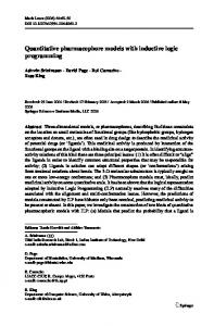
The F ratio, which is obtained by dividing the mean square regression by the mean square residual, is then transformed to a d statistic, and an appropriate sign is given. An alternative measure that combines the effect of the intervention on both the slope and the level was suggested by White et al. (1989). They proposed to calculate a regression equation for each phase and to compare the expected scores at the end of the experiment. A corrected standardized mean difference d can be calculated: Y * -Y * d = B *A , (12) SD _ with YB being the predicted score on the last occasion of the treatment phase, based on the treatment phase regres_ sion equation, Y B* the predicted score on the last occasion of the treatment phase, based on the baseline phase regression equation, and SD* the within-phase standard deviation around the regression lines. Instead of linear regression equations, it is possible that nonlinear time functions can be used to make predictions (Hershberger, Wallace, Green, & Marquis, 1999). Moreover, the point in time for which the score is predicted may be another point that is of interest scientifically (Hershberger et al., 1999). However, as we will demonstrate next, both the procedure of Allison and Gorman (1993) and that of White et al. (1989) are limited in describing the effect of an intervention. Two basic shortcomings can be identified. First, both kinds of effect size estimates depend on the length of the experiment. Second, different effects can lead to equal estimates of the effect size. Suppose Figure 1 represents the effects of an intervention for two cases. In the baseline phase, scores of both cases are approximated by a regression line with an intercept of 1.6 and a slope of 1. For the first case, there is no immediate effect on the level of performance, but there is an effect on the linear trend (the slope is doubled). For the second case, there is no effect on the linear trend, but scores are almost 14 points higher than would have been expected on the basis of the baseline regression line. From the figure, it can be seen that the length of the experiment can indeed influence the expected effect size estimates of Allison and Gorman (1993). If the two cases were not measured on the last three occasions, for both cases the residual variance would have been approximately the same, but the total variance would have been reduced (especially for Case 1). Therefore, the effect size estimates would differ from those obtained after the 20th occasion (Table 1). In the procedure of White et al. (1989), the estimate of the effect size also depends on the length of the experi-
4
VAN DEN NOORTGATE AND ONGHENA
Figure 1. The dependence of the measure of effect of Allison and Gorman (1993) and White, Rush, Kazdin, and Hartmann (1989) on the length of the experiment.
ment, in cases in which there is an effect of the intervention on the trend. In Figure 1, we see that if the treatment has a positive effect on the level and slope (Case 1), one can expect a larger effect size estimate if an experiment stops after 20 measurement occasions, rather than at the 17th occasion. For Case 2, in which there is no effect on the slope, the effect size measure, however, is not systematically affected by the duration of the experiment (Table 1). The arrows drawn in the figure indeed indicate that if the effect is evaluated at Occasion 20 instead of at Occasion 17, the distance between the regression line based on the baseline scores and the regression line based on the scores from the treatment phase gets larger for Case 1 but remains the same for Case 2. In addition, the example reveals that in both procedures, different effects can lead to equal effect sizes. Although both baselines are equal, the effect of the intervention is different in both cases. The effect of the intervention is initially larger for Case 2, but after a while, Case 1 seems to benefit most from the intervention. However, if residuals (for all 20 occasions) calculated using the baseline regression line are regressed on the phase 3 time phase interaction (Equation 8), the mean square regression and the mean square residual are approximately equal for both cases (467.50 and 10.16, respectively), giving equal Fs and equal effect size estimates in the Allison and Gorman
procedure (1993) (Table 1). Figure 1 also illustrates that the White et al. (1989) effect size estimates for both cases are very similar if evaluated after the 17th observation. Although it is true that additional data can make an observed effect more impressive, this is a matter that should be reflected in a statistical test or in a confidence interval of the effect size measure, not in the effect size measure itself. In order to describe the effect of an intervention,independently of the length of the experiment and without losing important information about the kind of effect, one single measure of effect size cannot suffice. Therefore, we propose an alternative procedure. Like Center et al. (1985– 1986), we suggest using a regression equation in which the scores are regressed on the phase, the trend, and the trend 3 phase interaction and calculating the regression coefficients on the basis of the ordinary least squares (OLS) criterion. However, instead of summarizing the effects by calculating the effect size on the basis of the F ratio, we suggest using the regression coefficients of this regression equation as measures of the effect. By using both coefficients b1 and b 3 from Equation 11 to describe the effect, both shortcomings described above can be avoided. Unfortunately, the regression coefficients are not necessarily comparable over studies. First, the time-related variable might be measured on dissimilar scales. In different studies, this variable can, for instance, be defined as
Table 1 Calculation of the Effect Sizes for the Two Fictitious Cases of Figure 1
Case 1 Evaluated after Observation 20 Evaluated after Observation 17 Case 2 Evaluated after Observation 20 Evaluated after Observation 17
Allison and Gorman (1993)
White, Rush, Kazdin, and Hartmann (1989)
Standardized Regression Coefficients
F(2,17) 5 46.00, d 5 4.65 F(2,14) 5 16.29, d 5 3.05
d 5 6.09 d 5 3.92
ˆ 5 0/bˆ * 5 0.61 b* 1 3 ˆ 5 0.20/bˆ * 5 0.53 b* 1 3
F(2,17) 5 46.00, d 5 4.65 F(2,14) 5 35.83, d 5 4.52
d 5 4.16 d 5 3.83
ˆ 5 4.16/bˆ * 5 0 b* 1 3 ˆ 5 4.27/bˆ * 5 20.06 b* 1 3
INTEGRATING EFFECT SIZES IN SINGLE-CASE RESEARCH the age in months, as the day number since the start of the experiment, or as the observation number. To make coefficients comparable, one must convert this time variable to the same scale. Second, the dependent variable can be measured on different scales. Often, however, it is realistic to assume that the scales of the dependent variable are linearly equatable (Hedges & Olkin, 1985), in which case the regression coefficients for the covariates can be made comparable over studies by dividing them by the rootmean squared error. Consequently, the corresponding (co)variance matrix of the estimates must be divided by the mean squared error. Note that if there is no linear trend, there is only one covariate, the phase indicator. Dividing the corresponding regression coefficient b1 by the root-mean squared error results in the standardized mean difference d. The use of the effect size measures we present thus simplifies to the use of the standardized mean difference if there are no linear trends. The standardized regression coefficients for the data from Figure 1 are also given in Table 1. It can be seen that these standardized regression coefficients are affected to only a very small degree by evaluating the effect after 17 observations, instead of after 20 observations. This influence of the length of the experiment is due only to the random fluctuation of scores around the regression lines. Moreover, it can be seen that using the standardized regression coefficients allows a more complete description of the effects. The Meta-Analysis of Standardized Regression Coefficients Because the standardized regression coefficients are comparable over studies, one can use them for a metaanalysis of the results of several studies. Since there are two measures for the effect in each study, we suggest performing a multivariate meta-analysis. Kalaian and Raudenbush (1996) presented a multivariate hierarchical linear model that can be used to perform a multivariate meta-analysis. On the first level, we have bˆ1 j = b1 j + e1 j and bˆ3 j = b3 j + e3 j ,
(13)
with bˆ 1j and bˆ 3j equal to the standardized OLS estimates of the regression coefficients for level change and slope change for case j and b1j and b3j equal to the “true” standardized regression coefficients for level change and slope change for case j. On the second level, b1 j = g 1 + u1 j and b 3 j = g 3 + u3 j .
(14)
On each level, residual terms are assumed to be multivariate normally distributed. Moreover, as is the case in a univariate meta-analysis, it is assumed that the Level 1 variance matrix is known. In practice, we use an estimate. This (estimated) covariance matrix of the regression coefficients can usually be retrieved when a linear regression analysis is performed with statistical software. Parameters can again be estimated with specialized hierarchical linear model software or by a general statistical package. For de-
5
tails about the estimation of the unknown parameters, we refer to Kalaian and Raudenbush (1996) and to the software manuals. To perform a multivariate meta-analysis, we do not need an estimate of all regression coefficients for all studies. Thus, the approach can still be used when, for one or more studies, data are analyzed using the regression model of Center et al. (1985–1986) but only the effect on the performance level or on the trend is reported. The model can again easily be extended to include study or case characteristics as covariates on the second level or to include other levels (for instance, separate case and study levels). An example. Marlowe, Madsen, Bowen, Reardon, and Logue (1978) designed an experiment to determine the relative effectiveness of teacher and counseling approaches in the reduction of disruptive or inappropriate classroom behavior. Inappropriate classroom behavior frequencies of 12 academically low-achieving, seventh-grade, black male students with a reported high rate of inappropriate classroom behavior were recorded. To evaluate counseling approaches, three groups of 4 students were randomly assigned to one of three treatment conditions: behavioral counseling, client-centered counseling, or no counseling. In Figure 2, time series graphs are shown, representing the frequencies of off-task behavior in the baseline phase and the interventionphase. During the second phase, eight 30-min counseling sessions were conducted for the behavioral (cases from first column) and client-centered (second column) counseling groups, while the no-contact control group (third column) continued baseline without treatment. We used the approach we presented above to combine the results from the time series graphs. Note that the cases differed from each other in the number of measurements in both phases, owing to missing values. After reconstructing the raw scores from the graphs, we performed separate ordinary regression analyses for each case, with the time variable defined as the day of observation minus the number of days in the first phase (10). The OLS regression coefficients, together with their covariance matrices, were standardized by dividing them by the root MSE and the MSE, respectively, and were used to perform a multivariate meta-analysis following the techniques of Kalaian and Raudenbush (1996). Calculations were done with the MlwiN software (Goldstein et al., 1998), assuming normal distributions for the residual terms. As was proposed by Kalaian and Raudenbush, the within-case residuals (e1j and e3j) were first made orthogonal with unit variance, using the Cholesky factorization (using the CHOL command in MlwiN). Setting up a multivariate model in MlwiN furthermore requires defining an additional lower level, without a Level 1 variation being specified, which is used solely to define the multivariate structure, using the dummies as predictors. We therefore used a three-level model, with the first level indicating the effect size measure, the second level the within-case level, and the third level the case level. The calculation of maximum likelihood estimates of the unknown parameters was done with the iterative generalized least
6
VAN DEN NOORTGATE AND ONGHENA
Figure 2. Time series graphs, representing the frequency of individual off-task behavior by day and condition, for the behavioral counseling group (first column), the client-centered counseling group (second column), and the no-contact group (third column). From “Severe Classroom Behavior Problems: Teachers or Counselors,” by R. H. Marlowe, C. H. Madsen, Jr., C. E. Bowen, R. C. Reardon, and P. E. Logue, 1978, Journal of Applied Behavior Analysis, 11, 62–63. Copyright 1978 by the Society for the Experimental Analysis of Behavior. Reprinted with permission.
squares algorithm of the program. The parameter estimates and the corresponding standard errors for the first model are presented in the first part of Table 2. The treatment seems to have a desired overall effect on both the level and the trend. We estimate that at the start of the second phase, the score decreases by more than one time the standard deviation of the scores around the regression lines. Moreover, the trend decreases by about one third of this standard deviation. On the basis of these overall parameters, one could predict, for a new case, the
evolution of the time series during the intervention phase, given his or her baseline scores. Using the Wald test and comparing the ratio of the parameter estimates and the corresponding standard errors with a standard normal distribution, we conclude that both gˆ1 and gˆ3 are significantly different from zero (z = 24.64, p =.00005, and z = 27.021, p < .00001, respectively). The estimated values of s 2u3 and su13 are zero, which suggests that cases do not differ from each other in the effect on the trend. The estimate of the between-case vari-
INTEGRATING EFFECT SIZES IN SINGLE-CASE RESEARCH ance of the coefficients indicating the effect on the level is 0.32. Yet, according to the Wald test with an alpha level of .05, this between-case variance is not significant (z = 1.6, p = .11). A small between-case variance estimate of a certain effect suggests that the effect is similar for all cases. This means that the estimate of the overall effect can possibly be a better estimate of an individualeffect than is the OLS estimate. Optimal estimates of the case-specific effects are obtained by using empirical Bayes techniques (Morris, 1983). These estimates are a weighted combination of the OLS estimates and the overall estimates. Although the empirical Bayes estimates are biased, using these estimates instead of the OLS estimates reduces the MSE (for a more elaborated discussion, see, e.g., Bryk & Raudenbush, 1992). In the example, the estimate of the variation of the treatment effects on the linear trend was zero. Therefore, the estimation of this effect is the same for each individual. This is not true for the effect on the level: Because the effect on the trend appeared to vary over cases, the estimated effects indeed vary around the overall effect, but are still “shrunk” to the overall effect. There is a tendency for the effects on the level to vary from case to case. A possible explanation is that the cases did not receive the same treatment: Whereas some cases received behavioral counseling, others received clientcentered counseling or no counseling. To explore the effect of the kind of treatment on the effect, we extend Equation 14 by regressing the effect on the level on dummies indicating the kind of treatment: bˆ 1 j = b1 j + e1 j and bˆ 3 j = b 3 j + e3 j , and b1 j = g 10 + g 11( behavioral) j + g 12 (client) j + u1 j and b3 j = g 3 + u3 j , (15) with (behavioral)j and (client)j equaling 1 if case j belongs to the behavioral counseling or the client-centered group, respectively, and 0 otherwise. While g10 of Equation 15 represents the mean effect on the level in the no-contact
group, (g10 + g11) and (g10 + g12) represent the mean effect on the level in the behavioral and client-centered counseling groups, respectively. The results are given in the second part of Table 2. The effect on the level in the behavioral counseling group appears to be more than twice the effect in the no-contact group (21.52 vs. 20.70; z = 22.65, p = .008), whereas the effect in the client-centered group is almost twice the effect in the no-contact group, although the difference is not statistically significant at the .05 alpha level (21.28 vs. 20.70; z = 1.87, p = .06). This conclusion is in line with the conclusion drawn by Marlowe et al. (1978) that “behavioral counseling, but not client-centered counseling was moderately helpful in reducing inappropriate classroom behavior” (p. 53). Our approach, however, gives a more detailed picture of the kind and the size of the effects. Finally, we note that the between-case variance of level effect disappeared. By taking the groups into account, the differences between the cases in the effect on the level thus are no longer larger than would be expected on the basis of the within-case variation alone. Finally, we note that because, in the example, the raw data are all available, there is no need to work with effect size measures but that one could combine the raw data immediately, using hierarchical linear models (e.g., Verbeke & Molenberghs, 1997). A two-level model could be used, in which the coefficients (on the first level, the measurement level) of the regression equation of Center et al. (1985–1986) vary from case to case (on the second level). We found that the results are comparable with the results of using the effect size measure approach. The Meta-Analysis for Other Single-Case Designs In the preceding, we assumed that data stem from studies with an AB phase design. In practice, AB phase designs are of limited use, because they do not manage to control for possible influences of historical events or other sources of influence that change over time. As the following suggestions will show, the use of hierarchical linear models is a comprehensive approach that can be translated, modified, or applied to the specifics of more complex designs.
Table 2 Results of the Meta-Analyses of the Regression Coefficients Model 1 Parameter
Estimates
Fixed Coefficients Effect on level g1 Overall 21.16 g10 No contact g11 Additional for behavioral counseling g12 Additional for client-centered counseling g3 Effect on trend 20.33 Effect on level Effect on trend Covariance level slope
7
(Co)variance Parameters s 2u1 0.32 s 2u3 0 s u13 0
Model 2 SE
Estimates
SE
0.25 – – – 0.047
20.70 20.82 20.58 20.33
– 0.26 0.31 0.31 0.035
0.20
0 0 0
8
VAN DEN NOORTGATE AND ONGHENA
The models without the trend parameter can be used without modification for other phase designs with two treatments, as well as for alternation designs, as long as there are no linear trends and the performance is similar in all A phases and in all B phases. For ABAB designs with dissimilar performance in the A and/or B phases, we propose to use the following Level 1 equation for case j: Yij = b 0 j ( block1) ij + b1 j ( phase)ij * ( block1)ij + b 2ij ( block2) ij + b3 j ( phase)ij * ( block2)ij + eij ,
(16) with (phase)ij being an indicator that equals 1 if occasion i is part of an intervention phase and 0 otherwise, and (block1)ij and (block2)ij being indicators that equal 1 if occasion i is part of the first or the second AB block, respectively, and 0 otherwise. Whereas b0j and b2j indicate the mean performances in the A phases, b1j and b3j can be interpreted as the effects in the first and the second blocks, respectively. If the OLS estimates of the coefficients b1j and b3j can be obtained, a meta-analysis of these estimates can be performed, using a multivariate model with the effect size estimates for the different blocks as the dependent variables. To take possible linear trends into account, Equation 16 can be adapted in a similar way as that discussed above. If phase or alternation designs are used to examine two or more treatments, one or more additional dummy variables can be included at the first level to indicate the treatment conditions. The results of a series of multiple baseline studies could be modeled by using a multivariate model, regarding the coefficients of the different response variables as different dependent variables, in case the same aspects are measured in the different studies. If the aspects that are investigated can rather be regarded as a random sample of possible aspects, an extra level can be included: Aspects are “nested” within cases. Distributional Assumptions In linear regression analysis, the estimation of the sampling distribution of the regression coefficients is based on the assumptions of independentlynormally distributed residuals and homogeneity of variance. The approximation of the sampling distribution of d is based on the same assumptions (Hedges, 1981). In addition, the approximation of the sampling distributions can be inadequate if based on a small number of observations. Moreover, although the sampling distribution of each regression coefficient divided by its standard error is a t distribution, in the present (multivariate) meta-analysis using hierarchical linear models, a (multivariate) normal sampling distribution of the effect sizes is assumed. Once more, this approximation is safe if the estimates are based on a sufficient number of observations. According to Hedges and Olkin (1985), these assumptions are often justified in group comparison studies. However, in single-case studies, the number of data points is often small (Huitema, 1985). Moreover, because in a singlecase experiment data are measurements stemming from the
same subject, serial dependence or autocorrelation may be present, violating the assumption of independence. Some claim that the existence of autocorrelation is a myth rather than a reality (e.g., Huitema, 1985), whereas others dispute this position (e.g., Matyas & Greenwood, 1991, 1997). The influence of serial dependency on the research results and possible corrections for autocorrelation often receive little attention, especially beyond lag 1 autocorrelation (Matyas & Greenwood, 1997). However, most quantitative or qualitative analyses of single-case data are not immune to the possible existence of serial dependency (Gorman & Allison, 1997; Matyas & Greenwood, 1991, 1997). Some techniques for time series data have been developed to test for autocorrelation or to account for autocorrelation (e.g., Box & Jenkins, 1976; Gottman, 1981). If raw data are available, the regression models we presented for the calculation of effect sizes could be adapted in similar ways to account for possible autocorrelation in the data. Unfortunately, these procedures often raise problems, because many data points are necessary to evaluate and estimate autocorrelation in the data (Busse et al., 1995; Jayaratne, Tripodi, & Talsma, 1988). If all raw data are available, the use of hierarchical linear models offers an elegant solution to the problem of autocorrelation. Indeed, instead of assuming a simple covariance structure, a more complex covariance structure can be assumed that takes into account a possible autocorrelation, as is discussed in Verbeke and Molenberghs (1997). Whereas in regular approaches the autocorrelation is estimated for each case separately, when a hierarchical linear model is used a possible autocorrelation is estimated by using all data. In the example described above, we found that for none of the 12 time series was the Durbin–Watson statistic for a first-order autocorrelation significant at a .05 level. Similarly, the estimate of the first-order autocorrelation coefficient in the hierarchical linear model analysis of the raw data was zero. Several alternativesare availablefor the meta-analysis of single-case data, with less restrictive assumptions about the sampling distributionsof the effect size measures. One can, for instance, use the binomial test, the Wilcoxon model, or the one-sample t test to construct a confidence interval around the mean effect size (Busk & Serlin, 1992), use study sample sizes instead of the reciprocal of the sampling variance as weights in the fixed effects techniques of Hedges and Olkin (1985) for calculating the mean effect size (Faith, Allison, & Gorman, 1997), or combine p values, possibly resulting from permutation or randomization tests (Onghena, 1994; Onghena & Van Damme, 1994). Unfortunately, all of these alternatives have the disadvantage of not taking into account a possible linear trend. Moreover, the procedures do not allow answering all the important meta-analytic questions, including an estimate and explanation of the true effect size variance. Conclusions We showed that the results of single-case studies could be combined by performing a (multivariate) meta-analysis on (standardized) regression coefficients. In cases in
INTEGRATING EFFECT SIZES IN SINGLE-CASE RESEARCH which there is no trend, this approach simplifies to a metaanalysis of standardized mean differences. Although the procedure outlined in this article does not solve all problematic aspects in the meta-analysis of single-case data, we tried to show that the procedure could give valuable information, which might be overlooked when other techniques are used. The approach presented is indeed very appealing for four reasons. First, interventions often do not have constant effects, but effects are conditional on time. In contrast to traditional approaches, the use of a multivariate meta-analytic model in cases of linear trends allows us to maintain the specific information that is given by each coefficient and to determine differential effects of a moderator variable on the level and on the slope. Whereas a positive effect of a moderator variable on the mean performance can be obscured by an opposite effect on the trend if one effect measure is used, this is impossible if both kinds of effects are represented by different measures. Using two measures of effect size also means that predictions can be made about the effect of an intervention on a future occasion. Second, the procedure easily extends to a meta-analysis of more than two regression coefficients—for instance, when the data for each case are modeled as a function of the time by means of a polynomial equation. Third, hierarchical linear models are very flexible and can be adapted according to the specific meta-analytic data set and the research interests by including covariates on the different levels or by including additional levels. The models presented furthermore include the possibility that true effect sizes vary partly in a predictable way according to study characteristics, partly randomly. The general hierarchical linear meta-analytic model indeed includes fixed and random meta-analytic models, combining the strengths of both kinds of models (see National Research Council, 1992). Finally, estimation procedures and user-friendly software are available to estimate and test the parameters of the models (for an overview, see Kreft & de Leeuw, 1998). In the estimation procedures, data are used efficiently in estimating unknown fixed and random parameters. Instead of the regression coefficients of the cases being estimated separately, empirical Bayes estimates of the individual coefficients use all data, resulting in more reliable estimates (Bryk & Raudenbush, 1992). REFERENCES Allison, D. B., & Gorman, B. S. (1993). Calculating effect sizes for meta-analysis: The case of the single case. Behaviour Research & Therapy, 31, 621-631. Box, G. E. P., & Jenkins, G. M. (1976). Time series analysis, forecasting and control. San Francisco: Holden-Day. Bryk, A. S., & Raudenbush, S. W. (1992). Hierarchical linear models: Applications and data analysis methods. Newbury Park, CA: Sage. Bryk, A. S., Raudenbush, S. W., Congdon, R. T., & Seltzer, M. (1988). An introduction to HLM: User’s guide, version 2.0 [Computer program]. Chicago: University of Chicago Press. Busk, P. L., & Serlin, R. C. (1992). Meta-analysis for single-case re-
9
search. In T. R. Kratochwill & J. R. Levin (Eds.), Single-case research design and analysis: New directions for psychology and education (pp. 187-212). Hillsdale, NJ: Erlbaum. Busse, R. T., Kratochwill, T. R., & Elliott, S. N. (1995). Metaanalysis for single-case consultation outcomes: Applications to research and practice. Journal of School Psychology, 33, 269-285. Center, B. A., Skiba, R. J., & Casey, A. (1985-1986). A methodology for the quantitative synthesis of intra-subject design research. Journal of Special Education, 19, 387-400. Cohen, J. (1969). Statistical power analysis for the behavioral sciences. New York: Academic Press. Faith, M. S., Allison, D. B., & Gorman, B. S. (1997). Meta-analysis of single-case research. In R. D. Franklin, D. B. Allison, & B. S. Gorman (Eds.), Design and analysis of single-case research (pp. 245-277). Mahwah, NJ: Erlbaum. Gingerich,W. J. (1984). Meta-analysis of applied time-series data. Journal of Applied Behavioral Science, 20, 71-79. Goldstein, H., Rasbash, J., Plewis, I., Draper, D., Browne, W., Yang, M., Woodhouse, G., & Healy, M. (1998). A user’s guide to MLwiN. London: University of London, Multilevel Models Project. Gorman, B. S., & Allison, D. B. (1997).Statistical alternatives for singlecase designs. In R. D. Franklin, D. B. Allison, & B. S. Gorman (Eds.), Design and analysis of single-case research (pp. 159-214).Mahwah, NJ: Erlbaum. Gottman, J. M. (1981). Time-series analysis: A comprehensive introduction for social scientists. Cambridge: Cambridge University Press. Hedges, L. V. (1981). Distribution theory for Glass’s estimator of effect size and related estimators. Journal of Educational Statistics, 6, 107-128. Hedges, L. V., & Olkin, I. (1985). Statistical methods for meta-analysis. Orlando, FL: Academic Press. Hershberger, S. L., Wallace, D. D., Green, S. B., & Marquis, J. G. (1999). Meta-analysis of single-case designs. In R. H. Hoyle (Ed.), Statistical strategies for small sample research (pp. 107-132). London: Sage. Huitema, B. E. (1985). Autocorrelation in behavioral research: A myth. Behavioral Assessment, 1, 107-118. Huitema, B. E., & McKean, J. W. (2000). Design specification issues in time-series intervention models. Educational & Psychological Measurement, 60, 35-58. Jayaratne, S., Tripodi, T., & Talsma, E. (1988). The comparative analysis and aggregation of single-case data. Journal of Applied Behavioral Science, 24, 119-128. Kalaian, H. A., & Raudenbush, S. W. (1996). A multivariate mixed linear model for meta-analysis. Psychological Methods, 1, 227-235. Kreft, I. G. G., & de Leeuw, J. (1998). Introducing multilevel modelling. London: Sage. Marlowe, R. H., Madsen, C. H., Jr., Bowen, C. E., Reardon, R. C., & Logue, P. E. (1978). Severe classroom behavior problems: Teachers or counselors. Journal of Applied Behavioral Analysis, 11, 53-66. Matyas, T. A., & Greenwood, K. M. (1991). Problems in the estimation of autocorrelation in brief time series and some implications for behavioral data. Behavioral Assessment, 13, 137-157. Matyas, T. A., & Greenwood, K. M. (1997). Serial dependency in singlecase time series. In R. D. Franklin,D. B. Allison, & B. S. Gorman (Eds.), Design and analysis of single-case research (pp. 215-243). Mahwah, NJ: Erlbaum. Morris, C. (1983). Parametric empirical Bayes inference, theory and applications. Journal of the American Statistical Association, 78, 47-65. National Research Council (1992). Combining information: Statistical issues and opportunitiesfor research. Washington, DC: National Academy Press. Onghena, P. (1994). The power of randomization tests for single-case designs. Unpublished doctoral dissertation, Katholieke Universiteit Leuven. Onghena, P., & Van Damme, G. (1994). SCRT 1.1: Single-case randomization tests. Behavior Research Methods, Instruments, & Computers, 26, 369. Pinheiro, J. C., & Bates, D. M. (2000). Mixed-effects models in S and S-plus. New York: Springer-Verlag.
10
VAN DEN NOORTGATE AND ONGHENA
Rosenthal, R. (1994). Parametric measures of effect size. In H. Cooper & L. V. Hedges (Eds.), The handbook of research synthesis (pp. 231244). New York: Russell Sage Foundation. Sheu, C.-F., & Suzuki, S. (2001). Meta-analysis using linear mixed models. Behavior Research Methods, Instruments, & Computers, 33, 102-107. Verbeke,G., & Molenberghs, G. (1997). Linear mixed models in practice: A SAS-oriented approach. New York: Springer-Verlag.
Wang, M. C., & Bushman, B. J. (1999). Integrating results through metaanalytic review using SAS software. Cary, NC: SAS Institute. White, D. M., Rusch, F. R., Kazdin, A. E., & Hartmann, D. P. (1989). Applications of meta analysis in individual-subject research. Behavioral Assessment, 11, 281-296. (Manuscript received March 16, 2001; revision accepted for publication March 19, 2002.)


![[PDF] Download Hierarchical Linear Models - Google Sites](https://m.moam.info/img/260x300/pdf-download-hierarchical-linear-models-google-sit_64785cda097c4796708cba0b.jpg)