Hierarchical Spatial Gossip for Multi-Resolution Representations in

Hierarchical Spatial Gossip for Multi-Resolution Representations in Sensor Networks Rik Sarkar, Xianjin Zhu, Jie Gao Department of Computer Science Stony Brook University Stony Brook, NY 11794-4400 {rik,

xjzhu, jgao}@cs.stonybrook.edu

Abstract

1. INTRODUCTION

In this paper we propose a lightweight algorithm for constructing multi-resolution data representations for sensor networks. We compute, at each sensor node u, O(log n) aggregates about exponentially enlarging neighborhoods centered at u. The ith aggregate is the aggregated data among nodes approximately within 2i hops of u. We present a scheme, named the hierarchical spatial gossip algorithm, to extract and construct these aggregates, for all sensors simultaneously, with a total communication cost of O(n polylog n). The hierarchical gossip algorithm adopts atomic communication steps with each node choosing to exchange information with a node distance d away with probability 1/d3 . The attractiveness of the algorithm attributes to its simplicity, low communication cost, distributed nature and robustness to node failures and link failures. Besides the natural applications of multi-resolution data summaries in data validation and information mining, we also demonstrate the application of the pre-computed spatial multi-resolution data summaries in answering range queries efficiently.

Distributed wireless sensor networks provide revolutionary ways to attain large scale, dense data collection and long-term environment monitoring. The immediate challenge is to develop efficient methods to extract, encode, and distribute information gathered by sensors, for both the robustness and survivability of data, as well as the flexibility and efficiency to answer user queries. In this paper we study the problem of constructing multi-resolution data representation in a sensor network to facilitate routing and answering multi-dimensional range queries. Our approach of processing data in a multi-resolution format follows the principle of fractional cascading that states: “a sensor knows a fraction of the information from distant parts of the network, in an exponentially decaying fashion by distance” [9]. This multi-resolution, locality-preserving representation is motivated by observations that sensors are typically monitoring a physical phenomena, which exhibits high correlation in both the spatial and temporal domain. Naturally information relevant to each node is decaying with the distance to this node. In the setup of this paper we have n sensors deployed uniformly and densely inside a region monitoring a continuous data field. We compute, at each sensor node u, O(log n) aggregates about exponentially enlarging neighborhoods centered at u. The ith aggregate is the aggregated data among nodes approximately within 2i hops of u. The specifics of aggregation techniques will be application dependent. For example, the aggregates can be the MAX/MIN or AVG, or more involved aggregates such as histogram [21], parameter estimations [24], or random linear projections used for compressed sensing and information recovery [20]. This multi-resolution scheme is inherently load-balanced. The storage requirement at each node is bounded by O(log n). We present a scheme to extract and construct these aggregates, for all sensors simultaneously, by a hierarchical spatial gossip algorithm. The total communication cost is O(n polylog n), only a small polylogarithmic factor of the cost for flooding or information aggregation at a sink, yet we obtain multi-resolution aggregation for each and every sensor node in the network. The multi-resolution data summaries provide a basis for information mining, data validation and efficient range queries. One of the major challenges in a sensor network is that nodes start with no idea of the big picture over the data field. Thus it is difficult for a node to assess whether its sensor reading is valid or not since detection of outlier or abnormality usually requires comparison with other sensor

Categories and Subject Descriptors C.2.2 [Computer-Communication Networks]: Network protocols—Routing protocols; F.2.2 [Analysis of Algorithms and Problem Complexity]: Nonnumerical Algorithms and Problems—Geometrical problems and computations

General Terms Algorithms, Design, Theory

Keywords Gossip, Multi-resolution representation, Order and Duplicate Insensitive Synopsis, Sensor Networks

Permission to make digital or hard copies of all or part of this work for personal or classroom use is granted without fee provided that copies are not made or distributed for profit or commercial advantage and that copies bear this notice and the full citation on the first page. To copy otherwise, to republish, to post on servers or to redistribute to lists, requires prior specific permission and/or a fee. IPSN’07, April 25-27, 2007, Cambridge, Massachusetts, USA. Copyright 2007 ACM 978-1-59593-638-7/07/0004 ...$5.00.

readings. In certain applications, the sensor field is deployed to detect events of interest to the owner. A sensor node often needs to decide, by itself, whether it holds interesting data or not. In some cases it is trivial, e.g., an unusually high reading by an acoustic sensor typically means activities in its vicinity. Sometimes this requires comparison with the average of sensor readings in an appropriate neighborhood. For example, the temperature threshold considered as ‘high’ in winter is different from that in summer. With the summarized data from each of its exponentially enlarging neighborhoods, a node has a basis against which its own reading can be compared, in order to spot local spikes which indicate data significance [22]. In addition, these partial aggregates can be used to support range queries injected from any node in the network. Queries for the aggregated value inside a geographical region can be answered by combining the pre-computed partial aggregates, without the necessity of examining each and every node in the geographical range. Thus both communication cost and query delay can be improved. The major contribution of this paper is the development of a light-weight algorithm for constructing multi-resolution data representations for sensor networks, as well as the application of multi-resolution data for range queries. In the remaining of this section we will survey related work on data processing in a sensor network and gossip-based algorithms. We will then give a quick overview of our solution for constructing and using multi-resolution data representation.

1.1 Information Processing in Sensor Networks Existing approaches for processing information in sensor networks can be classified into two main approaches: the standard sink model and distributed indexing and storage. In the standard sink model, data is delivered to the sink for out-of-network processing. Queries are disseminated from the sink to sensor nodes who will then report their readings. Data pruning and aggregation can be undertaken when data propagates up the tree to the sink (e.g., in TinyDB) [16]. The sink model assumes little or no in-network processing and most of the intelligence stays outside the network. The second approach uses in-network storage, builds distributed indices and stores partial aggregates to facilitate user queries. Examples of this category include DIMENSIONS [6, 5, 7], DIFS [10], DIM [15], and fractional cascading [9]. As storage devices such as flash drives become cheaper and smaller, the approach of using collective distributed storage becomes increasingly feasible. A distributed indexing structure typically involves a hierarchy to bring together data across different attribute space or spatial separations (e.g., quad-tree or kd-tree). Partial aggregates are computed bottom up for each node in the hierarchy. Queries take a drill-down approach and traverse the hierarchy to visit nodes holding relevant data for detailed information. Important considerations for distributed indexing and storage include how the partial aggregates are computed and who holds the aggregated data/indices. A straight-forward way is to take a hashing scheme and make certain nodes be responsible to hold aggregated data/indices on the hierarchy (e.g., in DIMENSIONS and DIFS). Special care is typically taken for nodes holding data at high levels of the tree to alleviate communication and query bottleneck [7]. The approach of fractional cascading in [9] belongs to the second category and tries to avoid the bottleneck created by

higher level nodes in the hierarchy. In [9], the sensor field is recursively partitioned by a standard quad-tree. Aggregates from each quad in the tree are computed and stored at all sensor nodes in the quad. Each node has the values of itself and aggregates of all the quads in which it resides. This improves data survivability and query efficiency as important information (e.g., the aggregates of larger regions) are naturally replicated more widely. Our multi-resolution representation can be considered as an alternative way to achieve fractional cascading. To see the difference of this paper with [9], instead of a fixed quad-tree partitioning, we keep the data summarization hierarchy of each node adaptive and centered on the node itself. Thus any two nodes will have slightly different world views at each scale, as their multi-resolution ranges differ, while two leaf nodes in a fixed quad-tree may share the same data of many highlevel quads. Another novelty of this paper is to investigate gossip-based algorithm to disseminate information and construct the multi-resolution data representation. A survey of gossip algorithms and applications in sensor networks is covered in the next subsection.

1.2 Gossip Algorithms Gossip algorithm is attractive for sensor networks, due to its distributed nature, robustness to network dynamics, and good load balancing. In a gossip algorithm each node picks, according to some underlying deterministic or randomized rule, another node and exchanges information with it [11]. There are two important aspects in a gossip algorithm: the gossip communication mechanism that decides which node to communicate with; and the gossip computation protocol that decides what data to exchange. In the literature two rules to select node to gossip with are prevailing. In uniform gossip, each node chooses to communicate with a randomly chosen node at each step [4]. In standard gossip on a graph, a node picks, according to a probabilistic distribution, one of its immediate neighbors in the graph [1, 24, 25]. Of particular relevance to our work is the spatial gossip algorithm proposed by Kempe, Kleinberg and Demers, where a node x selects a node y with probability proportional to 1/dρ , where d is the distance between x and y and ρ is some constant parameter [13]. The intuition of the spatial distribution complies with the principle of fractional cascading and our multi-resolution data representation. Data from a sensor node should, intuitively, be disseminated more to its nearby neighbors and less to far away neighbors. On top of the gossip communication mechanism, a gossip computation protocol specifies what information to be exchanged. In probably the simplest setting, information spreading [13], gossip is used to disseminate a piece of data from one node to the rest of the network. When two nodes communicate, the message is propagated. The protocol stops when all the nodes receive the message. More sophisticated information exchange protocols can be used to compute aggregations and global statistics among the gossip nodes. For the problem of distributed averaging [1], each node takes the average of the values of itself and its gossip partner. The algorithm converges when all nodes hold values close to the true average. Gossip-type protocols have also been developed in various settings to compute, in a distributed way, consensus [17, 1], various aggregates [12, 18], distributed linear parameter estimation [24, 25], spectral analysis [14] or

random linear projections of the data field for information compression and recovery [20].

1.3 The Challenge and Our Contribution To construct the multi-resolution data representation, we first note that simple flooding and aggregation from each node will incur too high communication cost – O(n2 ) since each node incurs a cost of O(n) to flood the network. In this paper we investigate gossip algorithms with almost linear communication cost. In our setting the metric we care most is the total communication cost of the gossip algorithm, which depends on two factors: the cost of communication for each iteration step, and the number of iterations for it to converge. Existing gossip protocols either assume that every two nodes can communicate with a unit cost (e.g., in peer-to-peer networks and distributed systems), or allow only immediate neighbors to gossip (e.g., in the standard gossip model). In our setting, we allow far away nodes to be chosen as gossip partners, and communication between them is performed by multi-hop routing. Thus the cost of each gossip step may involve any two nodes and have a higher cost if the nodes are far apart. This idea is also adopted in geographical gossip to reduce the communication cost of distributed averaging in a random geometric graph [4]. Under the objective of minimizing the total communication cost, the selection of gossip communication mechanism needs to balance two important factors. First, the fast convergence of a gossip protocol depends critically on the selection of gossip partners. Intuitively fast convergence requires information to be well mixed — one of the best is to select a random node in the network as the gossip partner. On the other hand, if we choose a random node to gossip in each iteration, the cost of communication with multi-hop routing is proportional to the distance to a random node in √ the network, which is roughly O( n) in a grid-like network with uniformly deployed sensors. To reduce the communication per each iteration, the best is to simply gossip with its immediate neighbors. But analysis of standard gossip on a random geometric graph or a 2-dimensional grid shows a slow convergence of roughly O(n2 ) gossip steps1 [23, 1], which is asymptotically the same order with that of naive flooding. The second challenge of the gossip algorithm in this paper, different from all the other gossip protocols, is on its multi-resolution nature. We would like information to be exchanged and mixed for fast convergence but also want to make sure that information does not travel too far and pollute the aggregates at other nodes. Thus the two conflicting considerations – fast convergence and restricted propagation range – also need to be carefully balanced. We propose to use a hierarchical spatial gossip algorithm that automatically takes care of all the issues we worried about above. Our hierarchical gossip algorithm proceeds in O(log n) phases. In phase i, we compute, for all sensor nodes, their respective aggregates in a roughly 2i neighborhood. This is achieved by a spatial gossip algorithm in a restricted range, where each node x picks, from nodes within distance 2i , a node y with probability proportional to 1/d3 , where d is the distance between x and y, 1 ≤ d ≤ 2i . Each phase stops after O(poly(i)) iterations, i ≤ log n. At 1 Here we use ‘gossip step’ to refer to the atomic operation of one node gossiping with its partner.

the end of phase i, we compute for each node u the aggregate of a subset of nodes Si (u) that contains all the nodes within distance 2i from u with high probability, and does not contain any node more than distance poly(i)2i apart. The total communication cost over all phases is bounded by O(n polylog n). Notice that this achieves a substantial improvement in terms of communication cost to the naive flooding approach and is only at most a polylogarithmic factor away from an obvious lower bound of Ω(n log n) for constructing the multi-resolution data representation2 . What is critical to the success of our hierarchical gossip algorithm is that we use order and duplicate insensitive synopsis (ODI-synopsis) [19, 3] to compute and represent the partial aggregates. The idea of an ODI-synopsis is that the same data can be aggregated multiple times but it is counted only once. Certain aggregates such as MAX/MIN are naturally ODI-synopses. ODI-synopsis for other aggregates such as COUNT and SUM/AVG are available, by implementation through MAX/MIN or boolean OR computations [19, 3, 2, 8]. ODI-synopsis combined with gossip algorithm removes trouble caused by the same data disseminated and aggregated multiple times. In addition, ODI-synopsis is helpful for range queries as we do not need to worry about overcounting resulting from partial aggregates from overlapping regions.

2. NETWORK SETUP In this paper we consider a network of n sensor nodes in a square. The sensor nodes are deployed with sufficient sensing coverage such that any unit disk centered inside the region contains at least 1 sensor node. Each sensor node knows its own location and generates a reading which is the sample of an underlying continuous and smooth data field at the location of this sensor. Notice that the above assumption guarantees sufficient coverage but does not prevent regions with dense node distribution. We can further improve the uniformity of the sensor sampling by clustering. We compute a set of clusterheads such that every two clusterheads are of distance at least 1 away and every node is within distance 1 of at least one clusterhead. The clustering can be easily implemented by a greedy and distributed algorithm. Each node checks its nearby nodes to see if there is a clusterhead within distance 1. Otherwise it will promote itself as a clusterhead. By local communication the nodes can select a subset of nodes as clusterheads as desired above. The set of clusterheads has bounded density. Every two clusterheads are at least distance 1 apart, as specified by the algorithm. Further, inside any disc of radius 2, denoted by D2 , there are at least 1 clusterhead — this is because any clusterhead outside this disc cannot cover the unit-radius disk D1 co-centric with D2 . Thus by the sampling assumption there is at least one node inside the unit disk D1 , whose clusterhead must be within D2 . Thus, without loss of generality we will assume in the following of the paper that: (i) any two sensor nodes are of distance at least 1 apart; (ii) any disk of radius 2 contains at least one sensor node. We assume that two sensor nodes can communicate with each other directly if they lie within a small distance of each 2 For each sensor node simply reading in their log n data summaries it requires a communication cost of Ω(n log n).

other. However, we do not enforce that the connectivity corresponds to a unit disk graph or any specific model. We assume that the deployment permits the existence of a multihop routing algorithm that can carry a message from node x to node y using at most O(dx,y ) hops, where dx,y is the Euclidean distance between the two nodes. For sensors uniformly deployed, simple geographical forwarding would suffice to find a path with length proportional to the Euclidean distance between them.

3.

SPATIAL GOSSIP

In this section we describe the hierarchical spatial gossip algorithm to compute multi-resolution data summaries for every sensor node.

3.1 Hierarchical Spatial Gossip We use a gossip mechanism where each node selects from a restricted neighborhood a node to gossip with and sends a message to it. The algorithm proceeds in phases. The phase i calculates for each node the aggregate of values inside a roughly 2i neighborhood centered at itself. The phases are completely independent so that phase i+1 starts fresh. Since we have a network of n nodes, with a lower bound on density, O(log n) phases are sufficient for the phase with the largest neighborhood to cover the entire network. For phase i, we adopt a restricted spatial gossip algorithm. We implement the selection of gossip partner with geographical routing. At each round, a node x chooses a location y ∗ in the sensor field with probability:  1 · (|xy ∗1|+1)3 , |xy ∗ | ≤ 2i ; ∗ π pi (x, y ) = 0, |xy ∗ | > 2i .

where |xy ∗ | is the Euclidean distance between nodes x and y ∗ . Notice that y ∗ is not necessarily the location of a sensor. x will send the information towards y ∗ and eventually reach the node y whose location is closest to y ∗ . Then y is x’s gossip partner and takes the information delivered by x. With the above gossip algorithm and the uniformity of sensors, the probability that a node x chooses a sensor node located at y (also denoted by y by slightly abusing the notation) is also proportional to 1/|xy|3 . Lemma 3.1. At phase i, let the probability that a node x gossips with a node y be qi (x, y). Then if 2 ≤ |xy| ≤ 2i + 2, qi (x, y) ≤ and if |xy| ≤ 2i − 2, qi (x, y) ≥

4 ; (|xy| − 1)3

1 ; 16(|xy| + 3/2)3

if |xy| ≥ 2i + 2, qi (x, y) = 0.

Proof. We compute the Voronoi diagram of all the sensor nodes (a partitioning of the region into cells such that all the points inside one cell are closest to the same sensor node) and only inspect the part inside the bounding square. In order for x to choose node y as its gossip partner, x must have chosen a location y ∗ that falls inside the Voronoi cell of sensor node y. Denote by V (y) the Voronoi cell of y, then R we have qi (x, y) = y ∗ ∈V (y) pi (x, y ∗ ). We now upper and lower bound the Voronoi region for y. V (y) is a convex region. The point on the boundary of

u y v

Figure 1. The Voronoi cell of a sensor node y is enclosed inside a disk of radius 2 and contains a disk of radius 1/2. V (y) furthest from y is realized at a Voronoi vertex (u in Figure 1), which has three sensors (including y) as its closest nodes. Thus the disk centered at u with radius |yu| has no other sensor nodes inside. Since any disk of radius 2 has at least one sensor node inside, |yu| < 2. Thus V (y) is enclosed by a disk centered at y with radius 2, denoted by D2 (y). On the other hand, the point on the boundary of V (y) closest to y, say v, is realized as the mid-point connecting y and one of its Delaunay neighbors (the sensors whose Voronoi cells are adjacent to that of y’s). Thus |yv| ≥ 1/2. Consider that y can be placed at the corner of the sensor bounding square. V (y) includes at least 1/4 of a disk of radius 1/2 centered at y. With the upper and lower bound of V (y), we will bound the probability qi (x, y). Take the point in V (y) closest to qi (x, y) = Rx, denoted by ∗w. |xw| ≥ |xy|2 − 2. Therefore 4 p (x, y ) ≤ pi (x, w)·π2 = 4/(|xw|+1)3 ≤ (|xy|−1) 3. y ∗ ∈V (y) i 1 Similarly, we have qi (x, y) ≥ 16(|xy|+3/2)3 . The above bound is valid when V (y) is completely within distance 2i from x, which is true if |xy| ≤ 2i − 2. If |xy| ≥ 2i + 2, then all points in V (y) are of distance 2i away. Thus y will never be chosen as x’s partner. qi (x, y) = 0.  We assume that all the nodes gossip in a synchronous way. At each clock tick, every node selects and shoots its information to its respective gossip partner. We consider each clock tick as a round. Once a node x chooses another node, say y, with distance at most 2i from it, x sends its current synopsis to y. y will incorporate the information it receives from x and maintain the aggregation of synopsis of its old value with the synopsis from x. Note that this is asymmetric as only node y updates its synopsis and node x keeps its current synopsis value. The asymmetry is an attractive feature as reliable round-trip multi-hop routing adds communication overhead and implementation difficulty. Denote by si,j (x) the synopsis at any node x after round j of phase i. The original value at x is thus given by s0,0 (x). After round j, each node updates its synopsis to be the aggregation of its synopsis at round j − 1 and all the values it received in this round. The value computed at node x at completion of phase i is denoted by si (x). All the aggregates in our scheme are order and duplicate insensitive synopsis. In particular, given a set of values S, an ODI-synopsis is an aggregate computed for values in S that remains the same no matter how many times one duplicates some values in S or what order the aggregation was performed. For example, MAX/MIN are naturally ODIsynopsis. ODI-synopsis for other aggregates such as SUM or AVG are available [19, 3, 2, 8] by essentially implement-

ing them by MAX/MIN or Boolean operations. We remark that some of the ODI-synopsis are probabilistic in nature. In this paper we often use MIN as the example, but the algorithm works with any ODI-synopsis. The use of ODI-synopsis is key to the success of the spatial gossip algorithm for constructing multi-resolution data representation. The insight is that aggregation by ODI-synopsis tremendously simplifies gossip computation protocol. Each node u keeps only a value s(v) which is the ODI-synopsis of the set of values it has received so far and does not keep the set of values in its original form. When one node u chooses to gossip with v, u sends to v its aggregate s(u) and v computes and keeps the ODI-aggregation of the synopsis of both u and v. s(v) ← s(u)⊕s(v), where ⊕ represents the aggregation function of the ODI-synopsis. This not only reduces the cost of transmission as only one aggregated value is delivered each step, but also guarantees that over-counting is eliminated although the same value may potentially be received multiple times. In short, with ODI-synopsis the model of gossip computation is the same as alarm spreading — each node starts with its own value and in each gossip step one node will send all the values it has received so far — but with reduced communication cost since only the aggregate (not the whole set of values) is delivered. When the algorithm stops, a node keeps the aggregate of all the values it has received. To make the analysis easier, we also denote by Si,j (x) the set of nodes whose values x should have received if we deliver all the original values instead of a synopsis in the gossip algorithm. In other words, si,j (x) is the aggregation of the values in the set Si,j (x). The set corresponding to the value si (x) at node x at the completion of phase i is denoted by Si (x). To summarize, there are at most O(log n) phases in the hierarchical spatial gossip algorithm. In phase i, every node executes O(i3.4 ) synchronous rounds. Each round consists of a single gossip operation performed by every node, and each phase consists of sufficient number of rounds so that nodes x and y that lie within a distance 2i of each-other obtain each-other’s values with high probability. Thus, at the end of phase i, any node has considerable information about values within a distance 2i from it. Thus the synopsis aggregate at each node has incorporated sufficiently many nodes within its 2i neighborhood. The gossip algorithm for each phase is very similar to the spatial gossip protocol proposed by Kempe et al. [13], except that we restrict the maximum range of gossip partners. This modification is to reduce the level of pollution such that a node does not receive information from nodes too far away, as will be made clear later.

3.2 Multi-resolution Representations In this section, we analyze the multi-resolution information computed by the algorithm described above. We show that if we stop the algorithm at phase i after j ∗ = O(i3.4 ) rounds, the synopsis kept at node x, i.e., the aggregated value of a set of nodes Si,j ∗ (x), captures the information is a roughly 2i neighborhood around x. Without loss of generally we denote by Si (x) and si (x) the respective values when j = j ∗ . Specifically, we show upper and lower bounds for the set of nodes in Si (x). Theorem 3.4 says that Si (x) includes with high probability each node within distance 2i from x.

Theorem 3.5 says that Si (x) does not include nodes O(2i i3.4 ) away for sure and with high probability does not include nodes with distance O(2i i2.4 ) or more away. Before we prove our main theorems, we first observe that when we run more iterations of the gossip algorithm, the amount of information each node gets is monotonically nondecreasing within a phase. Recall that Si,j (x) is the set of nodes whose values have reached x, after j rounds at phase i. Thus, Observation 3.2. Si,j (x) ⊆ Si,j+1 (x), for any i, j, x.

3.2.1 Lower bound We first show a lemma that bounds the rate of information propagation by the restricted spatial gossip algorithm. Intuitively the lemma says that after O(polylog d) rounds information at one node reaches a node at distance d with high probability. Lemma 3.3. In phase i, if the distance between nodes x and y is d ≤ 2i then Si,j (x) ⊆ Si,j+α (y) within α = O(log 3.4 d) rounds of iterations with probability at least 1 − O( 1d ). The proof is very similar with the proof in [13] that bounds the information spread rate in spatial gossip with necessary modification that additionally takes care of the restricted range. Thus we omit the details and refer the readers to [13]. This lemma shows that information propagates pretty fast in the network. Thus we can stop the algorithm in O(poly(i)) rounds for phase i, i ≤ log n, in order to collect information from almost all nodes inside the desired range 2i . Theorem 3.4. With probability at least 1 − O(1/2i ), the set Si,w (x) includes node y with |xy| ≤ 2i in phase i consisting of w = O(i3.4 ) rounds. Proof. Obviously x ∈ Si,0 (x). We apply Lemma 3.3 with d = 2i to obtain the theorem. This implies that in round i, any node collects information from each node in its 2i neighborhood with probability at least 1 − O(1/2i ). 

3.2.2 Upper bound

The subsection above shows that in phase i, any node receives the information within a distance 2i with high probability if we run the algorithm for O(i3.4 ) rounds. Now we show an upper bound that a node does not get information from nodes too far away. Thus the ‘pollution’ from far away nodes is bounded. Theorem 3.5. After k rounds of phase i, 1. Si,k (x) does not include nodes with distance d > k2i away from x, for sure. i

2. Si,k (x) does not include nodes with distance d > 3k2 i+1 away from x with probability at least 1−o(1/2k ), when i is greater than a sufficiently large constant. Proof. To make the analysis easier, we assume that we actually propagate, by the hierarchical spatial gossip algorithm, the list of values together with their source nodes. Initially each node has only its own value. Then they propagate to other nodes. We examine, for the value of a node u ∈ Si,k (x), the path it may take to get from u to x, denoted by P = {u, u1 , · · · , uℓ = x}. ℓ ≤ k. In round j, uj selects uj+1 as its gossip partner. Claim 1. The value of u cannot travel further than k2i because in any iteration, a gossip step can go as far as 2i at most and there are total k rounds.

Claim 2. Intuitively, for the value of u to reach a node x i that is distance d = (3+ε)k2 away (ε is very small) via a path i+1 of length at most k, it must make enough number of long jumps. We argue that the probability for this to happen is small. The following analysis is to make this intuition rigorous. First observe that the probability of a node uj choosing a node uj+1 of distance d′ > 2i /(i + 1) − 2 away is at most Z 2i 2r i+1 dr ≤ i−1 . 3 (r + 1) 2 i 2 /(i+1) Now consider a path P of at most k hops that starts from u and ends at x. Let k′ be the minimum number of steps of length 2i /(i + 1) or more in P . Then the minimum value of k′ satisfies the relation 2i (3 + ε)k (k − k )( − 2) + k′ (2i + 2) ≥ d = 2i . i+1 i+1 ′

When i is sufficiently large, k′ ≥ (2 + ε/2) ki . Therefore, for a k-hop path to reach node x, it needs to have at least k′ ´k′ ` ´` . long jumps, the probability of which is at most kk′ 2i+1 i−1 Thus, the probability that a k-hop path P does not have ′ k links of length 2i /(i + 1) or more is at least “ or `more ´ ` i+1 ´k′ ” k . 1 − k′ 2i−1 Now notice that for k rounds, the total number of possible k-hop paths that propagate the value of u is at most 2k . The probability that none of them reaches x is at least “ ` ´` ´k′ ”2k 1 − kk′ 2i+1 i−1 ´k′ k ` ´k′ ` ´` 2 ≥ 1 − 22k 2i+1 ≈ 1 − kk′ 2i+1 i−1 i−1 “ ” k 2/i ≥ 1 − 1/2k . ≥ 1 − (2(i+1)) 2ε/2 The last step is true when i is greater than a sufficiently large constant.  For a phase i, with k = i3.4 rounds, the probability that 3k the value at a node does not spread beyond a distance 2i i+1 3.4

is at least 1 − o(1/2i ). Thus with high probability Si (x) does not include nodes with distance O(2i i2.4 ) away.

3.3 Communication cost In this section we show that the communication cost of constructing the multi-resolution data representation is almost linear. Lemma 3.6. The communication cost incurred by any node in a single round of phase i is O(i). Proof. The expected distance to the gossip partner chosen by a node x is at most Z 2i r 2r 2+ dr ≃ O(i). (r + 1)3 0 Since the cost of routing to a node distance d away is O(d), the communication cost by any node in a round of phase i is O(i).  Theorem 3.7. The algorithm creates multi-resolution data as described above at every node using O(log4.4 n) rounds and total communication cost O(n log5.4 n). The storage requirement at each sensor node is O(log n).

Proof. In an n node network, with a constant lower bound on density, the maximum distance between any two nodes is O(n). Thus, the number of phases required by the algorithm is O(log n). Each phase i consists of O(i3.4 ) Plog n 3.4 ) = rounds. Thus, the number of rounds is i=1 O(i 4.4 O(log n). In phase i, at each round, a node uses a single message with an expected communication cost of O(i). Thus, the communication cost per node for the algorithm Plog n 3.4 is: ) = O(log 5.4 n). The total communication i=1 O(i · i cost is thus O(n log5.4 n). Notice that during the spatial gossip algorithm for phase i, each node at any time only keeps one value. The total storage requirement for each node is O(log n). 

3.4 Spatial gossip with metric ℓp For ease of explanation, we have described the concepts in terms of Euclidean distances, but the ideas extend to other ℓp distance measures. In ℓ2 measure, all points within a distance of d from point x form a circular disk of diameter d centered at x. Thus, the results of theorems 3.4 and 3.5 correspond to properties of data stored about disks of certain radii centered at each node in the network. For the type of rectangular range queries discussed in detail in the next section, it would be convenient to use ℓ∞ as the metric. In ℓ∞ , disks correspond to axis aligned squares that can be used to cover the query region.

4. RANGE QUERIES The pre-computed data summaries by the hierarchical spatial gossip algorithm can be useful in answering user queries about aggregates in large regions of the network with reduced cost. For example, the aggregate for the entire network is available at any single node. Similarly, it is possible to obtain probabilistic information about a large region of radius 2i by visiting a single node at its center. If the query requires better estimates of the aggregate, then it can be answered by making use of the different ODI synopses computed at different phases of the algorithm. Thus, the query response mechanism can adapt to the quality of estimate and restriction on pollution desired by the user. In the rest of this section we discuss a case where the user wishes to obtain with high probability the correct ODI synopsis of a rectangular region, without any pollution. The query consists of an a × b axis aligned rectangular area A, and a small probability δ. The response to the query is the ODI synopsis s corresponding to a set S, such that, for any node x, if x ∈ A then x ∈ S with probability at least 1 − δ, and if x ∈ / A then x ∈ / S. That is, no node outside the region A should be included in set S, and no node inside A should be excluded with a probability more than δ. Without loss of generality, we can assume that a ≤ b. By Theorem 3.4, after phase i, the ODI synopsis at any node x includes the value at any other node inside a disk of radius 2i with a high probability. For distances measured in the L∞ metric, this disk corresponds to a square of side 2 · 2i . We refer to such a square as a square of radius 2i (analogous to a disk of same radius), and use a set of such squares to cover the given query region. We denote by Bi (x) a square of radius 2i centered at node x. For a node y ∈ Bi (x), by Theorem 3.4, y ∈ / Si (x) with probability O(1/2i ). Corresponding to any square Bi (x), there is a square Gi (x) of radius ηi3.4 2i , for a proper constant η, such that for any node y ∈ / Gi (x), y ∈ / Si (x), by

Theorem 3.5. If the user query requires no pollution from outside the query region, the bigger square Gi (x) must be completely inside the query range. We refer to a square Bi (x) as a maximal piece if Gi (x) ⊆ A and Gi+1 (x) * A, and i as the maximal level of node x. Let Bp (x) be the largest maximal piece in A, then formally p = max{i : Bi (x) is a maximal piece}. x∈A

Then, we have a < η(p + 1)3.4 2(p+1) . 2 This implies that p = O(log a). Now we can collect the partial aggregates from these maximal pieces to answer the query. This can be done in a manner similar to that in [9] by starting at the boundary and spiraling inward accumulating synopsis for maximal pieces that together cover the entire region. Additionally, we must ensure that the probability of any node being excluded in the synopsis is small. ηp3.4 2p ≤

Query Range

Spiral

x Bi (x) Gi (x)

Figure 2. The spiral used for response for a given query region. Nodes are visited individually in the shaded region at the perimeter. The figure also shows the maximal square Bi (x) for a node x of maximal level i, and the corresponding pollution region Gi (x).

We use a spiral path that guarantees the required probability for every node in the query region. By Theorem 3.4, if a node is covered by a maximal piece Bi (·), the probability of it being included in the corresponding synopsis set Si (·) increases with the size of Bi (·). This implies that given a δ, nodes more than a certain distance (depending on delta) away from the boundary are covered by one or more maximal pieces that provide the required probability. Thus, our spiral starting at the boundary accumulates synopsis from all individual nodes up to this distance, and makes use of maximal pieces to obtain the synopsis for the rest of the region. Figure 2 shows a schematic representation of this idea. The following theorem gives the cost for such a computation. Lemma 4.1. Given a query (A, δ) where A is an a × b rectangular axis aligned query region, the query can be answered at a cost of O(max(a, b) log4.4 min(a, b) + max(a, b)(1/δ) log3.4 (1/δ)). Proof. For a node x, let dx be the distance of node x from the perimeter of the region A. If i is the maximal level of x, then ηi3.4 2i ≤ dx < η(i + 1)3.4 2(i+1) . This implies that all nodes of maximal level i occur in an annular rectangular region of inner boundary (b − 2η(i + 1)3.4 2(i+1) ) × (a − 2η(i + 1)3.4 2(i+1) ) and outer boundary (b−2ηi3.4 2i )×(a−2ηi3.4 2i ). The thickness of this annular rectangle is O(i3.4 2i ). To obtain the result with parameter δ, we start at the perimeter of region A, and spiral inward accumulating the synopsis s. At a distance ηd log3.4 d from the boundary, a maximal piece of level log d can be used, and the probability of a node at this level being missed by a maximal

piece is O(1/d). By the requirements of the query, it has to be ensured that δ = O(1/d). Thus, the spiral visits each individual node until the distance to the boundary reaches O((1/δ) log3.4 (1/δ)). At every node x, the synopsis is updated as s = s ⊕ s0 (x). The cost of such a path is O((a + b) δ1 log3.4 (1/δ)). After this point, the synopsis are updated according to maximal levels. At a node x of maximal level i, we set s = s ⊕ si (x), which is equivalent to the operation S = S ∪ Si (x). The lowest maximal level that we can use for the given query is γ = O(log(1/δ)). The cost incurred to process nodes at any maximal level i ≥ γ is O((a − i3.4 2i )i3.4 + (b − i3.4 2i )i3.4 ) = O(b · i3.4 ). The cost for the spiral covering all maximal levels i for γ ≤ i ≤ p is given by p X

i=log(1/δ)

O(b · i3.4 ) = O(bp4.4 ) = O(b log4.4 a).

Thus, the total communication cost for answering the query is O(max(a, b) log 4.4 min(a, b)+max(a, b)(1/δ) log3.4 (1/δ)).  Spatial gossip with no maximum range restriction. We note that the hierarchical spatial gossip for phase i makes only one change to the spatial gossip algorithm as in [13]. Essentially a node chooses its gossip partner with a maximum distance range 2i . This way we are able to restrict the amount of pollution from distant nodes. In the above range query, we make use of the fact that the data summaries do not include information beyond a certain distance threshold (claim 1 in Theorem 3.5), to answer queries with no false positive errors. For applications in which small false positive errors are not a problem, we can propose to use the single-phase spatial gossip algorithm to construct the multi-resolution data representations. Essentially, we just run the standard spatial gossip algorithm where each node chooses another node with distance d away with probability roughly 1/d3 . We run the algorithm for O(log3.4 n) rounds. During the algorithm, we keep the current aggregation value after round O(i3.4 ), as the data summary of the 2i -hop neighborhood. Notice that the probabilistic upper bound on pollution as the second claim in Theorem 3.5 still holds. Thus the ith data summary we compute has a large probability to include every value inside a 2i -hop neighborhood and not include values outside 2i i2.4 neighborhood. This alternative solution saves a factor of O(log n) in the total communication cost, at the cost of more pollution from far away nodes. For range query, a probabilistic solution with both small false positives and small false negatives can be obtained. In practice either variation can be adopted, dependent on application requirements. We evaluated and compared the gain of each variation in the simulation section. Error introduced by ODI synopsis. The analysis above considers the probabilistic error introduced by the gossip. ODI-synopses for aggregates such as SUM, AVG are probabilistic with small probabilities of error. Thus, the overall system error may incorporate this factor, which will depend on the actual ODI synopsis used.

5. SIMULATIONS In this section, we show that simulation results confirm our expectations on the properties of the hierarchical spatial

5.1 Total Communication Cost We simulated a grid network where the sensor nodes have a fixed transmission range 2. Nodes can communicate directly if they are within the transmission range of each other. Keeping the density of the network constant, we vary the number of nodes from 256 to 4900, and vary the size of the sensor field from 32 × 32 to 140 × 140. In the hierarchical spatial gossip, each phase i was terminated when at least (1 − 0.5/i) fraction of nodes in the entire senor field correctly computed the minimum value of resolution level i. This condition was found to provide a reasonable balance between fast information propagation and low pollution rates. Figure 3 shows the total communication cost in grid networks with various sizes. Naive flooding incurs dramatically higher cost, because in a network with n nodes, it requires O(n) transmissions for propagating one piece of data, and O(n2 ) transmissions in total. As expected, the hierarchical spatial gossip costs slightly more than the spatial gossip, but is still almost linear in the network size.

5.2 Effectiveness of Multi-Resolution Representation The approach of flooding the network is communication expensive. But with flooding we can compute the accurate multi-resolution data summaries by labeling each flood message with the location of its starting point. Thus, we only compare the effectiveness of multi-resolution representation of our approach with the single phase spatial gossip here. 6

5

x 10

4.5 4

Total cost

3.5

Hierarchical Spatial Gossip Spatial Gossip

3

Flooding

2.5 2 1.5 1 0.5 0 0

1000

2000

3000

4000

5000

Number of nodes Figure 3. Total communication cost in grid networks with various size.

We compare the standard spatial gossip with hierarchi-

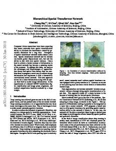
cal spatial gossip when they reach roughly the same state. For example, if round 15 of spatial gossip is the first round at which at least a fraction of (1 − 0.5/3) nodes correctly compute the aggregates of resolution level 3, then the states of the 15th round is comparable to phase 3 in hierarchical spatial gossip. The following simulations are conducted in a 128 × 128 grid network with 4096 sensor nodes. We take one piece of data s of the node located in the center of the network as a representative, and evaluate the entire process of its propagation. All other data is propagated in the same way. Intuitively, an ideal multi-resolution representation should compute aggregates at level i of almost all nodes belonging to Di , and little or no pollution beyond Di . The example of one execution in Figure 6 shows different phases of the propagation of s in the hierarchical spatial gossip. We can see that the information s is propagated within a restricted range in each phase and pollutes very few nodes beyond a certain distance. In the following, we use three measurements, viz., percentage of coverage, maximum distance and relative pollution, to compare the performance of our approach with the spatial gossip. Coverage. We define the percentage of coverage at distance d as the percentage of the number of nodes receiving s at distance d from the origin of s. In Figure 5, we show the percentage of coverage in an intermediate phase (phase 4) for both standard spatial gossip and hierarchical spatial gossip. The result confirms that there is a disk such that nodes within it receive the value with high probability. And the probability of a node outside this disk receiving the values falls sharply with the distance from the origin. 100 Hierarchical Spatial Gossip Spatial Gossip

90

Percentage of coverage

gossip. We compare our approach with the naive flooding and standard spatial gossip (single phase, with no restriction maximum range) for the total communication cost and the effectiveness of multi-resolution representation. We focus on evaluating the performance of our approaches at the algorithm level, and do not consider the underlying details, such as collisions and packet loss, at MAC and link layers. We use geographical routing in the simulations. Each packet transmitted only contains necessary location information and a piece of aggregate data of the source node. All simulations are done in C++ on a unit-disk graph model. For the simplicity of explanation, we denote the set of nodes within 2i distance from node x as Di (x). The aggregate of Di (x) is referred as the aggregate of resolution level i at node x. We compute the aggregate MIN as an example in the following simulations, other ODI-synopsis can be evaluated in the same way. All simulation results are averaged on 10 runs.

80 70 60 50 40 30 20 10 0 0

10

20

30

40

50

60

70

80

Distance Figure 5. Coverage of phase 4.

In the hierarchical spatial gossip, all nodes within a disk with radius 8 from the center receive s. The percentage of coverage decreases quickly as the distance increases, and goes below 10% beyond distance 30. The propagation quickly stops at distance 44.6. In standard spatial gossip, all nodes within a disk with radius 6 from the center receive s, but it pollutes the information at distant nodes up to a distance of 78, almost to the boundary of the network. Pollution. The small coverage in hierarchical spatial gossip implies low pollution rates. This is visible in figure 5. The single-phase spatial gossip always selects nodes from the entire network, thus it cannot guarantee a comparable restriction on pollution. We characterize and compare the pollution caused by the two approaches using two more criteria - maximum distance and relative pollution. We define the maximum distance of phase i as the distance between the center and the furthest node receiving s in phase i. The

10

80

9

70

8

Relative pollution

Maximum Distance

90

60 50 40 30 20

0 1

2

3

4

5

6

7 6 5 4 3 2

Hierarchical Spatial Gossip Spatial Gossip

10

Hierarchical Spatial Gossip Spatial Gossip

1 7

0 1

2

3

4

5

6

7

Phase Phase Figure 4. (i) Maximum distance reached in each phase. (ii) Relative pollution in each phase.

relative pollution of phase i is defined as the ratio of the number of nodes receiving s beyond Di (center) and the number of nodes receiving s within Di (center). Figure 4(i) shows the maximum distance reached at the end of each phase in both approaches. Since we simulate in a 128 × 128 grid network, the farthest point from the center is at a distance of about 90 units. In the hierarchical spatial gossip, the maximum distance increases relatively slowly with phases, while in the single-phase spatial gossip, the data often reaches distant nodes within the first few rounds. From Figure 4(ii), we can see that there is a big gap between the single-phase spatial gossip and the hierarchical spatial gossip in terms of relative pollution. The peaks are 9 and 2 respectively. Since we compare the states of the standard spatial gossip at the point of reaching the same state in the hierarchical spatial gossip, the number of nodes getting s within Di is roughly the same in both approaches. However, to build up the same level resolution, the singlephase spatial gossip would pollute data at about 4 times as many nodes beyond that level than the hierarchical spatial gossip. Conclusion. Efficient communication and sharp multiresolution representation are two conflicting goals. The naive flooding can obtain exact accurate aggregates but with high communication cost. The standard single phase spatial gossip is communication efficient, but it is possible that the information propagates to distant nodes before a sufficient number of nearby nodes gets the data. The hierarchical spatial gossip balances the above two goals by restricting the range of information propagation. Compared with the single-phase spatial gossip, it achieves a sharper multi-resolution representation with only a slightly higher communication cost.

6.

CONCLUSION

In this paper, we propose an efficient algorithm with a total communication cost of O(n polylog n) to extract and construct sharp multi-resolution data representations for sensor networks. We believe that the multi-resolution data summary is a fundamental data storage paradigm to equip each node with compact sketches of the global picture of the data field. As the future work we will explore more applications of multi-resolution data summaries for advanced data processing and validation, as well as efficient query evaluations. Acknowledgement. This work is supported by NSF CAREER Award CNS-0643687 and funding from Stony Brook’s

Center of Excellence in Wireless and Information Technology.

7. REFERENCES [1] S. Boyd, A. Ghosh, B. Prabhakar, and D. Shah. Randomized gossip algorithms. IEEE Transactions on Information Theory, Special issue of IEEE Transactions on Information Theory and IEEE/ACM Transactions on Networking, 52(6):2508–2530, June 2006. [2] E. Cohen. Size-estimation framework with applications to transitive closure and reachability. J. Comput. Syst. Sci., 55(3):441–453, 1997. [3] J. Considine, F. Li, G. Kollios, and J. Byers. Approximate aggregation techniques for sensor databases. In ICDE ’04: Proceedings of the 20th International Conference on Data Engineering, pages 449–460, 2004. [4] A. G. Dimakis, A. D. Sarwate, and M. J. Wainwright. Geographic gossip: efficient aggregation for sensor networks. In IPSN ’06: Proceedings of the fifth international conference on Information processing in sensor networks, pages 69–76, New York, NY, USA, 2006. ACM Press. [5] D. Ganesan, D. Estrin, and J. Heidemann. DIMENSIONS: Why do we need a new data handling architecture for sensor networks. In Proc. ACM SIGCOMM Workshop on Hot Topics in Networks, 2002. [6] D. Ganesan, B. Greenstein, D. Perelyubskiy, D. Estrin, and J. Heidemann. An evaluation of multi-resolution storage for sensor networks. In Proceedings of the first international conference on Embedded networked sensor systems, pages 89–102. ACM Press, 2003. [7] D. Ganesan, B. Greenstein, D. Perelyubskiy, D. Estrin, and J. Heidemann. Multi-resolution storage and search in sensor networks. ACM Transactions on Storage, 1(3):277–315, August 2005. [8] J. Gao, L. Guibas, J. Hershberger, and N. Milosavljevic. Sparse data aggregation in sensor networks. In Proc. of the 6th International Symposium on Information Processing in Sensor Networks (IPSN’07), April 2007. [9] J. Gao, L. Guibas, J. Hershberger, and L. Zhang. Fractionally cascaded information in a sensor network. In Proc. of the 3rd International Symposium on Information Processing in Sensor Networks (IPSN’04), pages 311–319, April 2004. [10] B. Greenstein, D. Estrin, R. Govindan, S. Ratnasamy, and S. Shenker. DIFS: A distributed index for features in sensor networks. In Proceedings of First IEEE International Workshop on Sensor Network Protocols and Applications, Anchorage, Alaska, May 2003. [11] S. M. Hedetniemi, S. T. Hedetniemi, and A. Liestman. A survey of gossiping and broadcasting in communication networks. Networks, 18(4):319–349, 1988. [12] D. Kempe, A. Dobra, and J. Gehrke. Gossip-based

(i) Phase 1

(ii) Phase 2

(iii) Phase 3

(iv) Phase 4

(v) Phase 5

(vi) Phase 6

Figure 6. Propagation of one piece of data of the node located in the center of the field.

[13]

[14]

[15]

[16] [17]

[18]

[19]

[20]

computation of aggregate information. In FOCS ’03: Proceedings of the 44th Annual IEEE Symposium on Foundations of Computer Science, pages 482–491, Washington, DC, USA, 2003. IEEE Computer Society. D. Kempe, J. Kleinberg, and A. Demers. Spatial gossip and resource location protocols. In STOC ’01: Proceedings of the thirty-third annual ACM symposium on Theory of computing, pages 163–172, New York, NY, USA, 2001. ACM Press. D. Kempe and F. McSherry. A decentralized algorithm for spectral analysis. In STOC ’04: Proceedings of the thirty-sixth annual ACM symposium on Theory of computing, pages 561–568, New York, NY, USA, 2004. ACM Press. X. Li, Y. J. Kim, R. Govindan, and W. Hong. Multi-dimensional range queries in sensor networks. In Proceedings of the first international conference on Embedded networked sensor systems, pages 63–75. ACM Press, 2003. S. Madden, M. J. Franklin, J. M. Hellerstein, and W. Hong. TAG: a tiny aggregation service for ad-hoc sensor networks. SIGOPS Oper. Syst. Rev., 36(SI):131–146, 2002. C. C. Moallemi and B. V. Roy. Consensus propagation. IEEE Transactions on Information Theory, 2007. to appear. D. Mosk-Aoyama and D. Shah. Computing separable functions via gossip. In PODC ’06: Proceedings of the twenty-fifth annual ACM symposium on Principles of distributed computing, pages 113–122, New York, NY, USA, 2006. ACM Press. S. Nath, P. B. Gibbons, S. Seshan, and Z. R. Anderson. Synopsis diffusion for robust aggregation in sensor networks. In SenSys ’04: Proceedings of the 2nd international conference on Embedded networked sensor systems, pages 250–262, 2004. M. Rabbat, J. Haupt, A. Singh, and R. Nowak. Decentralized compression and predistribution via randomized gossiping. In IPSN ’06: Proceedings of the fifth

[21]

[22]

[23] [24]

[25]

international conference on Information processing in sensor networks, pages 51–59, New York, NY, USA, 2006. ACM Press. N. Shrivastava, C. Buragohain, D. Agrawal, and S. Suri. Medians and beyond: New aggregation techniques for sensor networks. In SenSys ’04: Proceedings of the 2nd international conference on Embedded networked sensor systems, pages 239–249, New York, NY, USA, 2004. ACM Press. W. Wang and K. Ramchandran. Random distributed multiresolution representations with significance querying. In IPSN ’06: Proceedings of the fifth international conference on Information processing in sensor networks, pages 102–108, New York, NY, USA, 2006. ACM Press. L. Xiao and S. Boyd. Fast linear iterations for distributed averaging. Systems and Control Letters, 53:65–78, 2004. L. Xiao, S. Boyd, and S. Lall. A scheme for robust distributed sensor fusion based on average consensus. In Proceedings of the Fourth International Symposium on Information Processing in Sensor Networks, pages 63–70, 2005. L. Xiao, S. Boyd, and S. Lall. A space-time diffusion scheme for peer-to-peer least-squares estimation. In Proceedings of the Fifth International Symposium on Information Processing in Sensor Networks, pages 168–176, 2006.