power and a 100% fault coverage for non-fanout circuits. An extension for fanout circuits is also presented. 1 Introduction. In the production of VLSI and ULSI ...
Hierarchical Test Generation with Built-in Fault Diagnosis Dirk Stroobandt Jan Van Campenhout University of Ghent Department of Electronics and Information Systems St.-Pietersnieuwstraat 41, B-9000 Gent, Belgium dstr,jvc @elis.rug.ac.be �
�
Abstract A hierarchical test generation method is presented that uses the inherent hierarchical structure of the circuit under test and takes fault diagnosability into account right from the start. An efficient test compaction method leads to a very compact test set, while retaining a maximum of diagnostic power and a 100% fault coverage for non-fanout circuits. An extension for fanout circuits is also presented.
1 Introduction In the production of VLSI and ULSI components, testing takes considerable development time and effort. To reduce this effort, people have tried to make testing more efficient. The popular D-algorithm and its variations, P ODEM, FAN, S OCRATES, and other algorithms emerged [7]. Nowadays, more and more VLSI-components have built-in testing features. Still, even more efficient and accurate testing strategies are badly needed. With the increased complexity of components, many researchers have felt the need to exploit the hierarchy in systems architecture, producing separate tests for each module [1, 13, 14]. This way, the testing problem can be reduced considerably. In this paper, we present a method for automatic test pattern generation that uses the hierarchical nature of the components down to the gate-level. The test set itself is built hierarchically from tests for lower-level parts of the module. Our method also has the advantage that the test set obtained has excellent diagnostic capabilities. This means that, after applying the tests, one can immediately tell which parts of the module are defective. Unlike other diagnosis schemes (such as those using fault dictionaries [5], D IATEST [4] and others [2, 10, 18]), the extra tests needed for the diag�
Supported as Research Assistant with the Belgian National Fund for Scientific Research.
nosis are automatically added to the test set from the beginning. Yet, the test set with its diagnostic capabilities is kept very small due to an efficient compaction method [16, 17]. In the next section, the advantages of our method are highlighted and the improvements on the existing methods are pointed out. In sections 3, 4, and 5 the principles of the hierarchical test generation method and the compaction method are presented. Section 6 explains how the method can be expanded to also cover circuits with fanout lines. The results obtained can be found in section 7.
2 Hierarchical test generation and diagnosis Testing combinational circuits is not as difficult as testing sequential circuits. This is the reason why the well-known scan-path technique is used so often. All flip-flops are linked into one (or more) long shift register(s), called the scan-path, which can be tested independently of the rest of the circuit by applying a well-chosen bit stream. If this test succeeds, the flip-flop inputs can be considered as observable outputs of the combinational circuit and the flip-flop outputs can be used as controllable inputs. This way, the testing problem of sequential circuits equipped with a scan-path is reduced to a combinational one [19]. Our method can fully test and diagnose combinational circuits or circuits designed with the scan-path technique. With the classical ATPG algorithms, tests are generated by propagating and back-tracing fault-effects throughout the circuit. The aim is to find a set of input values that make a certain fault observable at the primary outputs. Typically, the circuit is considered as a whole and a lot of inputs must be given a value in each test. Moreover, tests are generated independently on the basis that a test should be generated for each fault not yet covered by a previously found test. On the other hand, each circuit may contain many identical elements. Many faults are thus in fact alike but they affect a different part of the circuit. It is tempting to take advantage of this. If it is possible to generate a test for a circuit out of known tests for each part of the circuit, then it is only
3 Initial test pattern generation 3.1 Modelling the connection hierarchy We consider purely combinational circuits, i.e., we assume that the circuit can be represented by a directed acyclic
X
A B
1
S
Y C Z
D
MUX2
A
2
B
4
out
3
Figure 1. Blocks 2 and 3 are pass-on blocks. Circuit inputs
Layer 2
Layer 1
Circuit outputs
B ...
B1 U0 ...
Bb+1
...
...
...
N2
...
N1
...
...
B2
...
Ii-1
...
I0 ...
Bb
Uu-1
Output block at level 0 Output block at level 1
...
necessary to find tests for low-level blocks. The test set for these blocks is small and easy to generate. It also has to be generated only once while it can be used in different parts of the circuit. In this paper, it is shown that this building of tests out of other tests is indeed possible, and a method is presented that makes efficient use of the inherent hierarchy within components. The basics of this method are similar to the ones used in [6]. Starting with small tests for each submodule, a test set is generated for the whole circuit by building the test set level by level. Most test generating methods are only concerned with fault coverage. The fault coverage is defined here as the percentage of detectable faults of a given fault model that can be detected by tests from the test set. The fault model is a list of faults that should represent as much as possible real defects. Considerable effort has been spent on finding efficient fault models. A detectable fault is a fault of the model that would be detected if all possible tests would be applied to the circuit. Note that some faults are non-detectable due to the circuit structure itself. Since it is impossible to find a test for a non-detectable fault, those faults should not be included in the fault coverage. With tests based on fault coverage only, we can only tell whether or not a fault of the fault model occurred. However, if one wants to know precisely which fault caused the failure of a test, one has to apply a diagnostic procedure. Diagnosing faults after application of all tests can be difficult and time consuming, because the diagnostic capability of test sets is usually very low, thus demanding extra tests. This overhead could be avoided by taking the diagnostic resolution into account while generating tests. The possibility of fault diagnosis is important for improving process yield. Consider a programmable gate array consisting of a number of cells, each with their own functionality. In a go/no-go testing procedure, one stops when a fault occurs. Then the whole component is useless and should be discarded. In a testing environment with diagnostic features, the defects can be located. If we can exclude the defective part so that the user can never use it, then the rest of the component may still satisfy the requirements. The component is not totally lost and the yield could be higher. Such schemes to improve yield have been presented in [8] and [11]. With the recent trend towards extremely complex programmable arrays and wafer scale integration, it will probably be necessary to achieve a reasonable yield by making partly defective components (partly) usable.
Output block at level k
Figure 2. The structure of a high-level block.
graph. The logic gates of the circuit are represented by the nodes in the graph. Each node belongs to a sub-graph, called Layer. The number of the layer to which a node belongs, corresponds to the longest path from the node to an output node. In order to make all paths from a given node to the output nodes equally long, we introduce dummy pass-on nodes. In the circuit description, pass-on blocks are introduced as illustrated in figure 1. All output nodes are in layer 1 and will be collected into one output block. Starting from this output block as hierarchical level zero, the entire circuit can be given a hierarchical structure. The output block at hierarchical level is formed by adding to the output block of level ���� the nodes of the preceding internal layer (figure 2). At each hierarchical step, the new output block is considered as one new node, and the numbers of all preceding layers are decreased by one since the paths between each node and the outputs become shorter. With this, each high-level block � consists of two layers. Layer 1 contains one output block ��� �� , which may itself be a high-level block, and layer 2 has an arbitrary number of basic input blocks � ,...,� � . These are multiplexers, and-gates, or-gates, or any other single-output module. The inputs of block � are connected to the inputs of the layer 2 blocks through a net block . The outputs of the layer 2 blocks are connected to the inputs of block � � ��
through net block �� . In � fanout is possible, in �� a 1to-1 relationship between connected lines is assumed.
3.2 Test generation for the layer 2 blocks Our test generation method has been developed for the single stuck-at fault model, extended by bridging faults at adjacent input lines of layer 2 blocks. However, the method is applicable for other fault models as well. The D-notation [19] is used, so the possible values on signal lines are 0 (low), 1 (high), (low, but high on error), and (high, but low on error). The values and will be called pseudo-logic values. The faults on the lines � and � will be denoted as ����� (stuck-at-0 fault on line � ), ��� � (stuck-at-1 fault on line � ), � ����� � (bridging fault between lines � and � with logical zero dominating), � � ��� � (bridging fault between lines � and � with logical one dominating), � � � (bridging fault between lines � and � with the value of line � dominating), and � � � (bridging fault between lines � and � with the value of line � dominating). With this fault model, a test set is generated for each layer 2 block as if it were a stand-alone circuit. This is done by writing down all possible combinations of input values and verifying which faults of the fault model apply to each combination. This is feasible since the number of inputs of the layer 2 blocks is low. The inputs that could have a different value under faulty conditions are given pseudo-logic values if the fault is observable at the output. A pseudologic value on a signal line (for a particular test) indicates that faults can be propagated through the signal line and are observable at the output for this test. In table 1, the complete test set is given for a 2-to-1 multiplexer. This table is called the test table. For each test, it gives the necessary input conditions, the value of the output, and the matching faults. The input vector � = (��� ,..., ����� ), where � is the number of inputs, can contain both logic or pseudo-logic values. The output always has a pseudo-logic value because the stuck-at fault at the output line is always observable. The set ��� of the matching faults constitutes the fault cover of the test ��� . Because all input combinations are used, all the detectable (digital) faults are present in the test set and the fault coverage of the test set is thus 100%. For diagnostic purposes, we need another table besides the test table. We call it the diagnostic table. In this table, each row consists of a vector � = ( � � ,..., ��� � ), with � the number of tests in the test set, and a fault set � . The components of � indicate which tests possibly fail, and � is the set of faults identified by � (One of the faults in � occured if all tests with � �"! � fail). For each combination of tests,
�#!%$'& � �1032 $ 4 � 5 0;: ( �*) +�,.-� ./ 6( 5 ) +879-��9/ This way, all faults are identified by exactly one combination of failing tests. If the fault set of a combination is empty, this combination can be discarded from the diagnostic table (except for the situation where no fault occurs and no test fails).
Test #
��� � , >�� � < � � , ��� � , >�� � , � � � , � �?��� � < < < � � , ��� � , >�� � , �A� , �A� , < < �B����� , �� � , �E� , �B��� � ��� � , >�� � < < < ��� , ��� � , >�� � , �E� , �B��� � , �C�A� , � � �?����� < ��� , ��� � , >�� � , � � � , � �?��� � ����� , >�� �
Table 1. Test table of the 2-to-1 multiplexer. The number of rows in the diagnostic table, J , is bounded by � the number of faults in the fault model and therefore JLKNM . The diagnostic table of the 2-to-1 multiplexer is given by table 2. This table distinguishes between all faults of different equivalence classes. While performing the tests, the defective line can be found immediately by checking which tests fail and comparing the results to the information in the diagnostic table. For instance, if only test � � fails then we see from line OLF of the diagnostic table that there is a bridging < fault between lines and � with the logical one dominating.
4 Compaction of the test set Since we want to combine test sets of layer 2 blocks into a test set for a higher-level block, it is essential to reduce the size of all lower-level sets to their absolute minimum. The goal is to reduce the test set while retaining its full diagnostic power, as exhibited by table 2. In this table, it is obvious that one could eliminate some of the tests (columns), while retaining a unique encoding of each row. For instance, test � � can be omitted. Hence, we want to identify the largest subset of columns that we can eliminate while retaining unique row encoding. Equivalently, we seek the smallest set of tests that uniquely encodes the individual fault sets. Since a unique encoding requires the distinguishability of all diagnostic row pairs, we can transform the selection problem into a generic column covering problem [9] by considering a new table. In this table, the rows correspond to diagnostic row pairs, and the columns to the tests that can make the distinction between the pair members. However, � this table has size O(J � ). Hence, we have worked out a direct solution of the encoding problem, using a recursive division of the diagnostic table (which only has size O( JP� )). By choosing one test, we divide the table into two sub-tables. The first one contains only those rows that have a 0 in the column of the chosen test, the second sub-table has the rows
Row #
OL�
Test combination vector �
� �
O
O�� O D OLF O G O H O I O � O��
0 0 0 0 0 0 0 0 0 0 0 1 1
O �
O
O �
�
� �
� D
� F
� G
� H
� I
0 0 0 0 0 0 0 0 0 1 1 1 1
0 0 0 0 1 1 1 1 1 0 1 0 0
0 0 0 0 0 0 1 1 1 0 0 0 0
0 0 0 1 0 0 0 0 0 0 0 0 1
0 1 1 0 0 1 0 1 1 0 0 0 0
0 0 1 1 0 0 0 0 0 1 0 0 1
0 1 0 0 0 0 0 0 1 0 0 0 0
Fault set � fault free
��� � < � � , � � � ��� � < �B��� � < � �?��� � , �A� < ��� � , �A� < �B��� � >�� � � �?��� � < � � , � � � ��� � >�� �
Table 2. Diagnostic table of the 2-to-1 multiplexer.
that contain a 1 in that column. This division process is based first on “essential” tests, next on the “most informative” test. An essential test is a test that is needed because it is the only one that differentiates between two faults. Omitting this test would result in the inability to make a difference between the two faults. For instance, test � I is necessary to < make a difference between faults �B����� (row O I ) and >���� (row O ). The most informative test is a test that divides the table in as good as equal sub-tables. A division on the basis of test � � results in one sub-table of length 6 and one of length 7 (nearly equal length). For the example of the 2-to-1 multiplexer (see table 2 for the diagnostic table), test � � is chosen first (essential and most informative), resulting in two sub-tables. The first table contains rows O � , O , O�� , O D , O , O , and O � . The second one gets O F , O G , O H , O I , O , and O � . These two tables are divided further by choosing at each recursion level one essential test. If there are no essential tests left, the “most informative” test is chosen. This results in the test set � � , � G , � D , � , � I of all essential tests augmented by the set �8F , ��H of (at that moment) most informative tests. The division process terminates when all tables consist of only one row. Note that in this example, we need seven out of eight tests to maintain full diagnosability (i.e., unique row encoding). However, when larger test sets are compacted, the compaction ratio is much higher. In [16] it is shown that this compaction method gives a near-optimal test set with the same diagnostic features as the original test set, with all the faults still detectable, and all this with significantly fewer tests (high compaction ratio). This can also be seen in the results presented in section 7.
�
�
�
�
�
��
�
5 Combining tests for higher levels With the compacted and non-compacted test tables of the layer 2 blocks and the compacted test table of the final output block, we now present a method to generate the test set for higher-level blocks. The method must at least take into account all tests in the compacted test table of each block to maintain full diagnosability and a 100% fault coverage. When designing the tests for the higher level block, we try to limit ourselves to using tests from the compacted test set. However, we must ensure that 1. The outputs from layer 2 blocks are made observable through block � � �� , preferably by activating this block with a test from its compacted test set. This implies that the output of the layer 2 block, routed via net block
� , forms part of a test for block � � �� . If the test set of block � � �� has a 100% fault coverage, this requirement is always met. 2. The outputs from layer 2 blocks should suffice for the controllability of block � � �� , i.e., one should be able to generate the compacted test set of block � � �� through tests on blocks �� ,..., � � . Here it may be necessary not to limit oneself to compacted test sets for the layer 2 blocks. Because the layer 2 blocks have very small test tables, this is not a big problem. The search method is represented by the pseudo code of procedure COMBINE in figure 3. This procedure combines all tests from the compacted test set of each layer 2 block with other tests to create a test set for the higher level block � . The block currently under examination is called block �"� . For the search of appropriate tests in the other layer 2 blocks, the procedure BACKTRACE is called. This procedure recursively visits each layer 2 block � ,..., � � other than block � � . In each block, a test is searched that is compatible with the input values already defined by a test on a previous block. If, in a certain block, such a test cannot be found, then the procedure returns to the previous level of recursion (to the last treated block) and tries another test. This mechanism continues until a good test is found for all blocks or no test combination is possible satisfying the requirements. If no fanout is present in net then the condition marked with an in procedure BACKTRACE is always met and a test will always be found eventually. In that case, the final test set has a 100% fault coverage. The procedure BACKTRACE is also presented in figure 3. It takes three parameters: the number of the next layer 2 block � � that has to be searched, the number of the layer 2 block � � that is to be skipped and a third parameter that holds the result of the search operation on return to the procedure COMBINE.
�
procedure COMBINE for (all layer 2 blocks �� ) for (all tests ��� of the compacted test table of block �� ) � Combine test ��� with a test � � from the compacted test table of block � �� . The input values of test ��� must be compatible with the output value of test ��� and must have a pseudo-logic value to ensure that the output value of block �� is observable at the primary outputs.; Call the recursive procedure BACKTRACE (1, � ,false) to look for an appropriate test on the other layer 2 blocks.; � procedure BACKTRACE ( NEXTBLOCKNO , SKIPBLOCKNO , TESTFOUND ) if (NEXTBLOCKNO = ����� or TESTFOUND = true) � set TESTFOUND = true; return � if (NEXTBLOCKNO = SKIPBLOCKNO) � BACKTRACE ( NEXTBLOCKNO +1, SKIPBLOCKNO , TESTFOUND ); return; � for (all tests ��� of the test table of block �� with � = NEXTBLOCKNO) � if ((��� sets the output of �� to the value needed to control the inputs of � ��� as in test ��� ) and (the input values corresponding to test ��� do not conflict with previously assigned input values) ) BACKTRACE ( NEXTBLOCKNO +1, SKIPBLOCKNO , TESTFOUND ); if (TESTFOUND = true) break; � �
return;
�
Figure 3. Pseudo-code of the search method (the condition marked by an is only needed when fanout is present in net and it is the only condition that can prevent the procedure BACKTRACE from finding a test eventually).
After the tests of all blocks � through � � are handled, the stuck-at faults on the input lines are added to all tests that detect them and again the test compaction algorithm is used to obtain a compact test set for the high-level block with high diagnosability of the faults on its internal lines. In procedure BACKTRACE, we try all possible tests of the compacted test set of block � � �� . This is necessary to obtain a high diagnosability figure. If we would only consider one applicable test of block � � �� , a lot of faults in different blocks would collapse into the same diagnostic row pair. It is guaranteed that the procedure will find at least one applicable test combination under the restriction that net block � does not contain fanout lines ([16]) and that all layer 2 blocks allow both logic values at their output. For this, we only need the compacted test tables in procedure COMBINE. In order to find an applicable test, even though fanout is present, we use the full (uncompacted) test table of the blocks � � for the search in procedure BACKTRACE. This way, more tests will be applicable and the chance that the fanout lines impose too many restrictions, is a lot smaller. Still, with fanout lines, we cannot guarantee that the procedure will find applicable test combinations. In section 6 we will therefore expand the method for use when fanout creates problems. Note that this method inherently rests on the controllability and observability of all the blocks within the circuit (a necessary requirement for testability [15]).
6 Expanding the scope One can prove that for non-fanout blocks, the previous method is able to find a compact test set with a fault coverage of 100% [16]. The method can also distinguish between all faults in the same layer 2 block. Full diagnosability is not guaranteed because it is possible that (non-equivalent) faults in two different blocks have the same diagnostic row and thus the distinction cannot be made. However, the test sets obtained by using this method showed that, when we try every possible combination of tests in the examined block with every test in the output block (compacted test sets), such collapsing faults are rare. Now, if we want to support fan-out lines in net block , problems can occur because there are some restrictions on the values of the connected lines, resulting in the possibility that the right test combination is never found in procedure BACKTRACE. In that case, some test of the examined block is not present in the overall test table. This means that some faults may no longer be covered by the test set. Experiments show that this is frequently the case when an input line leads to a layer 2 block and a pass-on block at the same time, as is illustrated by figure 4. Suppose we have a test of block 1 that sets line to 0. Suppose that only one test in block 3 can be combined with the test of block 1 and that this test sets the output of block 2 to 1. In this case, we cannot find a test of block 2 that meets the restrictions because there is a conflict.
level
Figure 4. Fanout lines can cause problems.
The examined test of block 1 cannot be added to the overall test set. If this test was essential for a fault (i.e., no other test can detect the fault), that fault will not be covered by the test set. Yet, there could well exist a test able to detect the fault. We found the following solution for this problem. First, the presented method is used to generate test patterns for a slightly different circuit. This circuit is the same as the original except that we provide extra input lines for the fanout lines. With the extra input lines, again there is no fanout and the method generates a test set with a 100% fault coverage and nearly complete diagnostic capacity. The test set for the original circuit is then obtained from the test set generated above by dividing this set into two parts. The first part contains all tests that have the same initial logic value on the lines connected with the fanout line. These tests are compatible with the real circuit and represent an initially correct test set. The other tests have at least one line, coming from a fanout line, with a different value. Based on these tests, new tests are generated for the real circuit by changing alternatively the value of one of the conflicting lines. These new tests are propagated through all blocks up to the outputs of the circuit under test. Because we have a full test table of all layer 2 blocks and a block description of all high-level output blocks in terms of other layer 2 blocks, this propagation is straightforward. A backtracing mechanism then changes the necessary values from logic to pseudo-logic values and adds the faults (also listed in the database of each block) to the test table. This finally gives us the full description of the new test (input value combination and corresponding faults). These new tests are added to the initially correct tests and the total test set is compacted. The way we deal with fanout lines still does not guarantee a fault coverage of 100% but the results obtained with it are very good. Because we start with the most promising tests (obtained with the method for the adjusted circuit), we find almost all faults with very little overhead. Also the diagnosability remains the same. If, however, some faults are no longer detected by the changed test set, then a classical ATPG algorithm could be used to generate a test for these few faults. This way, we can obtain a 100% fault coverage. By supplying a few extra tests one can also obtain a 100% diagnosability. ATPG algorithms for tests that make a differ-
BOTTOM LEVEL 0 LEVEL 1 LEVEL 2 LEVEL 3 LEVEL 4 LEVEL 5 A LEVEL 5 B LEVEL 5 C LEVEL 5 D LEVEL 6 A LEVEL 6 B TOP
�
���
���
���
� �
� �
O��
4 3 3 5 2 0 3 5 5 8 9 9 0
168 271 341 460 531 701 897 1109 1339 1579 1859 2147 2379
0 0 0 0 0 0 1 10 0 9 7 5 0
17 22 22 27 28 36 50 69 81 97 106 130 121
100 100 100 100 100 100 99.7 97.1 100 98.1 99.1 99.3 100
98.2 80.0 83.3 87.3 71.5 86.5
100 100 99.5 99.7 99.0 99.2 97.8 97.5 95.8 94.4 94.7 96.5 96.4
� : � � � :� � � � : ��� � : � � ����: M � ���� : ��� � :� �
Table 3. Results of the test generation and diagnosis method. For the numbers marked with an , the maximum number of different tests was previously compacted in parts. So the real compaction percentage is higher.
�
ence between non-equivalent faults are discussed in [2]. Because only a few tests have to be added, this step takes only a small amount of the total time needed to generate the tests.
7 Results The test generation method presented in this paper has been implemented in C code to generate a test set for a custom designed FPGA (Field Programmable Gate Array) [3]. This FPGA contains 16 RLBs (Routing and Logic Blocks), which provide both functionality and routing resources to the whole chip. One RLB contains 29 4-to-1 multiplexers, 10 2-to-1 multiplexers, 1 and-gate, 1 or-gate, 74 D-flipflops (contain the programmable values), 2 S-flip-flops, and 7 buffers with a total of 3062 transistors. The RLB has been divided into 9 levels, two of which were divided into parts because of the high percentage of fanout lines. This extra division had a negative effect on the results as can be seen in table 3. In this table, � is the number of fanout lines (counted at the input), ��� is the number of detectable faults in the fault model up to this level, ��� is the number of extra tests necessary to obtain a 100% fault coverage, � � is the total number of tests after compaction, ��� is the obtained fault coverage before supplying extra tests, ��� is the percentage of compaction of the test set (i.e., 100% - � � / maximum number of different tests generated on that level), and O�� is the diagnosability (i.e., number of diagnostic rows / number of non-equivalent faults. This is the so-called diagnostic power [12]).
Up to LEVEL 4 we obtain a fault coverage of 100% with the presented method, even though fanout is present. The diagnosability stays above 99%. This means that for fewer than 1% of all the faults we cannot distinguish between two faults with the obtained test set. It is possible to increase the diagnosability figure to 100% by supplying a few extra tests. In table 3 the power of the compaction method is also illustrated. We obtain a very high compaction ratio for each level without loss of fault coverage or diagnostic power. For levels 5 and 6, we needed to supply a few extra tests in order to obtain a 100% fault coverage. This was mainly due to some implementation problems. We believe that a better implementation (without the need to divide these two levels into separate parts) would give even better results.
8 Conclusions In this paper we have presented a new test set generation method for ASICs with the following properties: it generates a (nearly) minimal test set; it has a very high fault coverage for the detectable faults of the fault model (single stuck-at faults and bridging faults on adjacent lines of the same layer 2 block). A 100% fault coverage is guaranteed for circuits without fanout lines; it offers the possibility of a very high diagnosability for all non-equivalent faults. The first results obtained with this method are promising. The hierarchically building of test sets reduces the number of calculations because tests for identical gates in different parts of the circuit are generated only once. The possibility to optimise the test set within each level of hierarchy results in a very compact test set throughout the generation process. This compact test set though has immediate diagnostic features.
References [1] J. D. Calhoun and F. Brglez. A framework and method for hierarchical test generation. In 1989 International Test Conference, pages 480–490, August 1989. [2] P. Camurati, D. Medina, P. Prinetto, and M. Sonza Reorda. A diagnostic test pattern generation algorithm. In 1990 International Test Conference, pages 52–58, 1990. [3] J. Depreitere, H. Neefs, H. Van Marck, J. Van Campenhout, R. Baets, B. Dhoedt, H. Thienpont, and I. Veretennicoff. An optoelectronic 3-D field-programmable gate array. In R. W. Hartenstein and M. Z. Serv´ıt, editors, Field-Programmable Logic. Architectures, Synthesis and Applications, volume 849 of Lecture Notes in Computer Science, pages 352–360. Proceedings of the 1994 Workshop on Field Programmable Logic and Applications, Springer-Verlag, September 1994.
[4] T. Gr¨uning, U. Mahlstedt, and H. Koopmeiners. DIATEST: A fast diagnostic test pattern generator for combinational circuits. In IEEE International Conference on Computer-Aided Design: Digest of Technical Papers, pages 194–197, Santa Clara, CA, USA, November 1991. [5] J. Kato, T. Shimono, and M. Kawai. Fault diagnosis based on post-test fault dictionary generation. In 1989 International Test Conference, page 940, August 1989. [6] D.-W. Kim, J. H. Schlag, and J. L. A. Hughes. Digital CMOS VLSI test generation: a divide-and-conquer algorithm. In IEEE International Symposium on Circuits and Systems, volume 3, pages 1097–1100, May 1992. [7] T. Kirkland and M. R. Mercer. Algorithms for automatic test pattern generation. IEEE Design and test of Computers, vol. 5 (no. 3): pages 43–55, June 1988. [8] V. Kumar, A. Dahbura, F. Fischer, and P. Juola. An approach for the yield enhancement of programmable gate arrays. In IEEE International Conference on Computer-Aided Design: Digest of Technical Papers, pages 226–229, Santa Clara, CA, USA, November 1989. [9] D. Lewin and D. Protheroe. Design of Logic Systems, chapter 10. Chapman & Hall, UK, second edition, 1992. [10] H.-T. Liaw, J.-H. Tsaih, and C.-S. Lin. Efficient automatic diagnosis of digital circuits. In IEEE International Conference on Computer-Aided Design: Digest of Technical Papers, pages 464–467, 1990. [11] P. K. Rhee, J. H. Kim, and H. Y. Youn. A novel reconfiguration scheme for 2-D processor arrays. In IEEE International Conference on Computer-Aided Design: Digest of Technical Papers, pages 230–233, Santa Clara, CA, USA, November 1989. [12] E. M. Rudnick, W. K. Fuchs, and J. H. Patel. Diagnostic fault simulation of sequential circuits. In 1992 International Test Conference, pages 178–183, September 1992. [13] Z. Sahraoui, P. Six, I. Bolsens, and H. De Man. Search space reduction through clustering in test generation. In B. Werner, editor, Proceedings of EURO-DAC ’95, European Design Automation Conference with EURO-VHDL, pages 242–247. IEEE Computer Society Press (Los Alamos, California), September 1995. [14] T. M. Sarfert, R. Markgraf, E. Trischler, and M. H. Schulz. Hierarchical test pattern generation based on high-level primitives. In 1989 International Test Conference, pages 470–479, August 1989. [15] J. Savir. Good controllability and observability do not guarantee good testability. IEEE Transactions on computers, vol. C–32 (no. 12): pages 1198–1200, December 1983. [16] D. Stroobandt. A demonstration circuit for opto-electronic interconnections, 1994. Engineering thesis, University of Ghent (in Dutch). [17] G.-J. Tromp. Minimal test sets for combinational circuits. In 1991 International Test Conference, pages 204–209, October 1991. [18] J. A. Waicukauski and E. Lindbloom. Failure diagnosis of structured VLSI. IEEE Design & Test of computers, pages 49–60, August 1989. [19] B. R. Wilkins. Testing digital circuits, an introduction. Van Nostrand Reinhold, UK, 1986.