BAE Systems (BA21) and Smiths Group (SMIN21); and two banks: Barclays (BARC81) and Royal Bank of Scotland (RBOS81). As in earlier work [1], we denote ...
Hierarchical Topological Clustering Learns Stock Market Sectors Kevin A.J. Doherty, Rod G. Adams, Neil Davey and Wanida Pensuwon Department of Computer Science, University of Hertfordshire, AL10 9AB, UK e-mail: {K.A.J.Doherty,R.G.Adams,N.Davey,W.Pensuwon}@herts.ac.uk Abstract—the breakdown of financial markets into sectors provides an intuitive classification for groups of companies. The allocation of a company to a sector is an expert task, in which the company is classified by the activity that most closely describes the nature of the company’s business. Individual share price movement is dependent upon many factors, but there is an expectation for shares within a market sector to move broadly together. We are interested in discovering if share closing prices do move together, and whether groups of shares that do move together are identifiable in terms of industrial activity. Using TreeGNG, a hierarchical clustering algorithm, on a time series of share closing prices, we have identified groups of companies that cluster into clearly identifiable groups. These clusters compare favourably to a globally accepted sector classification scheme, and in our opinion, our method identifies sector structure clearer than a statistical agglomerative hierarchical clustering method. I. INTRODUCTION There has been recent interest in the discovery of structure in stock markets from an analysis of the time series of closing prices of the shares traded within the market [1][2]. The methods for discovering structure are generally based on the minimum spanning tree (MST) of the correlation of the logarithmic return of the day-on-day price change. These works show that share closing prices carry both valuable and detectable economic information, which may be useful in producing a theoretical description of financial markets and explaining the economic factors that affect specific groups of stocks. These are important claims, and motivated the work presented here. Individual share price movement is dependent upon many factors, but there is an expectation for shares within a market sector to move broadly together. We are interested in discovering if share closing prices do move together, and whether groups of shares that move together are identifiable in terms of industrial activity. In addition to clustering those companies that exhibit a similar share closing price history, we are also interested in discovering and extracting hierarchical structure within data. Our approach uses a neural-inspired clustering algorithm to learn a topologypreserving mapping of the data whilst maintaining a history of the learning process, which gives the hierarchical structure. We use the Euclidean norm combined with normalised data for the measurement of distance. Thus, the application of our hierarchical clustering method, combined with data normalisation of financial time series data, is the contribution of this paper.
II. HIERARCHICAL TOPOLOGICAL CLUSTERING In this section we outline TreeGNG, an unsupervised learning method, which produces hierarchical classification schemes, based on a topology representing network. TreeGNG incrementally learns a topology-preserving mapping of the data space with the algorithm outlined in section A, and produces a hierarchical representation of this mapping with the method outlined in section B. A. Growing Neural Gas The Growing Neural Gas (GNG) algorithm is a neuralinspired clustering algorithm that produces clustering schemes with no hierarchical structure [3]. GNG incrementally adapts, grows and prunes a graph structure consisting of nodes and edges. The nodes of the graph are of the same dimensionality (D) as the input space. The topological neighbours of a node are defined as the nodes that are adjacent in the graph. The GNG algorithm is initialised with two nodes randomly positioned in ℜD connected by a single undirected edge. The edges in the graph have a corresponding age, and new edges have an age of zero. At each adaptation step, the nodes “compete” to represent an input drawn at random from the input data set. The winning node is updated with the standard competitive learning rule [4] at a rate ηw, and all of its topological neighbours are updated at a reduced learning rate, ηL. The age of edges incident to the winning node are incremented, and the squared error is added to a local error for the winning node. If the winner and second closest node are topological neighbours, then the age of the edge forming the neighbourhood is reset to zero. If these two nodes are not topological neighbours, then a new edge is inserted into the graph between the nodes. Every iteration, all of the edges with an age greater than αmax are deleted. If this results in a node having no incident edges, then the node is deleted. If the number of adaptation steps is equal to an integer multiple of the growth-parameter λ, then a new node is inserted into the graph between the node with the greatest local error, and its topological neighbour with the greatest local error. The new node is initialised with a local error equal to the mean of its topological neighbours, and the local errors of these neighbours are decreased by α. The algorithm continues to process input vectors until the user-defined stopping criteria are satisfied. The GNG algorithm has many user-defined parameters; including the maximum number of nodes N, the learning rates ηw and ηL, the maximum edge age αmax, the local error decay
R
(i)
R
(ii)
R
(iii)
(vi)
R
A
B
A
(vii)
R
R A
B
A
C
(viii)
R
B
B
A
B
A
(v)
R
(iv)
B
C
Fig. 1. The TreeGNG Growth Mechanism. The shaded cloud-like areas are the regions of the input space from which the input data are randomly selected. In (i), GNG is initialised with two nodes joined by a single edge. The tree consists of a single root node R. In (ii), following a period of standard GNG dynamics, the dashed edge is marked for deletion in the GNG graph. As the edge is deleted in (iii), the graph splits and node R grows two children A and B to represent the increase in the number of graphs. A growth window is opened for node R. After a further period of GNG dynamics, the growth window for node R closes (iv) and any subsequent graph splitting will result in tree growth under nodes A or B. In (v), the dashed edge is marked for deletion, and in (vi), the edge is deleted producing child growth beneath node A. The growth window for node A is opened. In (vii), the dashed graph edge is marked for deletion, and the natural tree growth should occur as children of node C, but because the growth window for node A is still open, the new node is inserted as a child of node A, i.e. a sibling of node C. Following a period of GNG dynamics and the growth of two children of B, the final tree structure is shown in (viii).
rate α, the global error decay rate d, and the growth phase timer λ. In [5] it was reported that GNG converges rapidly, and that the quality of the clustering has little dependence on the network parameters. The results of our own evaluation of GNG agree with these findings.
graph. As the GNG node and edge insertion routines grow the graph structure, the root node maintains the pointer to the revised graph. As a part of the GNG dynamics, edges are aged, and old inactive edges are periodically deleted. A graph edge deletion event can result in a graph splitting into two sub-graphs, and it is this splitting that initiates tree growth. As a graph splits into two sub-graphs, a growth window is activated for the tree node that pointed to the original graph. Any subsequent splitting of the sub-graphs that occurs whilst this window is open, results in nodes being inserted into the tree as siblings of the sub-graph tree node; when the window closes, any subsequent graph splitting results in nodes being inserted into the tree as children of the sub-graph tree node. Without this window, the tree growth is event driven and always produces a binary tree. As is shown in [6] and [7], the
B. TreeGNG By maintaining a time audit trail of the graph connectivity, we can uncover hierarchical structure within a data set. In earlier work [6][7], we presented the TreeGNG algorithm. In TreeGNG, we use GNG as the partitioning algorithm and generate a tree structure based on the time history of the graph connectivity (Fig. 1). The standard GNG algorithm begins with a graph of two nodes joined by a single edge, and the TreeGNG tree is initialised with the root node pointing to this (i)
(ii)
R A
b
C
B
c
a
(iv)
R
AB A
A B
a
(iii)
R
b
AB B
C
c
ab
R C
C
c
ab
c
Fig. 2. The TreeGNG Pruning Mechanism, also demonstrating how the algorithm can recover from poor decisions made in the construction of the tree. In (i), TreeGNG has formed a poor tree structure in which tree nodes B and C are siblings. With the standard GNG dynamics, it is likely that an input would cause graphs a and b to merge as the dashed edge is inserted. To maintain the correct tree structure, this requires tree nodes A and B to merge (ii). In (iii), as the graphs a and b are merged, then a new tree node AB (pointing to the merged ab graph) is inserted into the tree as a child of the common ancestor of A and B. The dashed tree nodes (A and B) are removed from the tree. Finally, in (iv), the intermediate singleton tree node between R and C is removed. Subsequent GNG dynamics are likely to cause graph ab to split into two graphs, and tree node AB would grow two children to reflect this change. The resultant tree structure is more representative of the data than the original tree shown in (i).
length of time the growth window is open influences the shape of the tree. A short period yields a binary tree, whilst an extremely long period yields a flat clustering with no hierarchical structure. Wide ranges of intermediate values yield more representative tree structures. Tree pruning (Fig. 2) occurs following an edge insertion event occurring in the GNG graph, merging two graphs into a single super-graph. The merging graphs may not be siblings in the tree, and so a new tree node pointing to the new super-graph is created as a child of the common ancestor of the two merged graphs. The tree nodes pointing to the original two merged graphs are removed from the tree. Finally, singleton tree nodes are removed. In the resultant tree, only leaf nodes of the tree maintain pointers to the GNG graph structures. III. STOCK MARKET STRUCTURE Financial markets are complex systems [8]. To aid the understanding of the core business activities of the companies within these complex systems, the constituent companies within a stock market are assigned to one-of-many possible sectors. One universally accepted classification scheme is the FTSE Global Classification System (Fig. 3) which is based on the division of a market into Economic Groups, Industrial Sectors and Industrial Sub-sectors. This system has been used to classify company data for over 30,000 companies from 59 countries [9]. A committee of experts performs the classification of companies, subject to the rules outlined in [10]. The aim of the classification is to allocate a company to the sub-sector that most closely describes the nature of its business. It is against this FTSE Global Classification System that we present the discussion of the clustering results presented in the sequel. IV. STOCK MARKET DATA
TABLE I FTSE GLOBAL CLASSIFICATION SCHEME
Economic Group Industrial Sector 00 Resources
04 Mining 07 Oil & Gas
ANTO, RIO BG, BP, SHEL
10 Basic Industries
11 Chemicals 13 Construction 15 Forestry & Paper 18 Steel & Other Metals
JMAT HNS, WOS
20 General
21 Aerospace & Defense BA, RR, SMIN 24 Diversified 25 Electronic 26 Engineering TOMK
30 Cyclical Consumer Goods
31 Automobiles & Parts 34 Household Goods
40 Non-cyclical Consumer Goods
41 Beverages 43 Food Producers 44 Health 47 Personal Care 48 Pharamceuticals 49 Tobacco
ALLD, DGE, SCTN ABF, CBRY, ULVR
52 General Retailers
BOOT, DXNS, GUS, KGF, NXT, MKS HG, WTB BSY, DMGT, EMA, EMG, PSON, REL, RTR, WPP BNZL,CPI,HAS,REX,RTO BAA, BAY, EXL
50 Cyclical Services
53 Leisure & Hotels 54 Media 58 Support Services 59 Transport
63 Food & Drug Retailers MRW, SBRY, TSCO 67 Telecommunication BT, CW, VOD
70 Utilities
72 Electricity 77 Utilities - Other
80 Financials
81 Banks
90 Information
93 Information 97 Software & Computer SGE
10 Economic Groups 36 Industrial Sectors
30,000 Companies
Fig. 3. The FTSE Global Classification System. The hierarchical classification consists of 10 groups which follow a general economic theme, 36 sub-ordinate groups (Industrial Sectors) that follow a general industrial theme, and 102 further sub-ordinate groups (Industrial Subsectors) that follow specific industrial themes. This classification scheme has been applied to over 30,000 companies in 59 countries [9]. Table I details the 10 Economic Groups and 36 Industrial Sectors, along with the FTSE 100 constituents with their respective Industry Sector.
RB, SN AUN, AZN, GSK
60 Non-cyclical Services
The FTSE 100 is an index of the top 100 capitalised blue
102 Industrial Sub-sectors
Constituents
SPW, SSE SVT, UU
BARC,HSBA,LLOY, RBOS,STAN 83 Insurance RSA CGNU, LGEN, PRU 84 Life Assurance 85 Investment Companies III 86 Real Estate BLND, LII, LS 87 Speciality AVZ, SDR 89 Investment Entities
An extract from the FTSE Global Classification System [9], showing the Economic Groups and Industrial Sectors - the 102 Industry Subsectors are omitted for brevity. The constituents list the stock tick symbols for the 73 companies that have been members of the FTSE 100 for the period 1st January 1995 to 30th April 2005.
chip companies in the UK, and is recognised as the measure of UK stock market performance [11]. The closing price for the constituent companies of the FTSE 100 were collected for the period 1st January 1995 to 30th April 2005; a total period ( T )
V. RESULTS The critical TreeGNG network parameters were based on the results of experiments reported in [6] and [7]. As a reminder, the data set consisted of 73 feature vectors of dimensionality 2696. For these data, we used a TreeGNG growth window (q.v. Fig. 1) of 3 epochs. The GNG nodes were inserted every 20% of an epoch (i.e. node insertion rate λ = 15), and edge deletion occurred when an edge aged to greater than 10% of an epoch (i.e. edge deletion age αmax = 7). The remaining GNG parameters were set to a configuration we have successfully used on many data sets (ηw = 0.1, ηL = 0.01, α = 0.5, and d = 0.99). We trained the network for 30 epochs with the number of network nodes, N, equal to 50 and
6 7
12
5
4
8 3
Closing Price (£)
of 2697 trading days. We only examined the 73 companies that were members of the FTSE 100 throughout this period. The list of companies examined in this paper, along with tick symbols (a unique abbreviation of the company name) and Industrial Sector are shown in Table I. As in earlier work [1], we denote Pi(t) as the closing price of company i, (i = 1,…,73) on day t, (t = 1,…,T), and the logarithmic return, Si, on the share price after time interval ∆t (where in this paper ∆t is one trading day) as Si(t)=ln(Pi(t+∆t))– ln(Pi(t)). This produced a 2696 dimension feature vector per company, with no missing values. In [12] and [13], it was shown that a Euclidean distance measure with normalised data is an effective method of recovering cluster structure. Data normalisation, or ranging, is the linear transformation achieved by the division of the range (or spread) of a variable. For the stock market data examined in this paper, it is possible to normalise the data either i) daily, with the division by the range of S for all the companies at time t, or ii) normalise the logarithmic return Si(t) against the range of Si in T. The results presented in this paper are based on the logarithmic return of Si(t) normalised by the range of Si, with a Euclidean metric.
2
4
1 1998
2004
1998
RSA83
1998
2004
CGNU84
2004
BA21
11
25
6 9 15
4
7
5
2
5 1998
2004
SMIN21
1998
2004
1998
BARC81
2004
RBOS81
Fig. 4. Share closing price history during the period 1st January 1995 to 30 April 2005 for two insurance companies: Royal Sun Alliance (RSA83) and Aviva (GCNU84); two industrial manufacturing companies: BAE Systems (BA21) and Smiths Group (SMIN21); and two banks: Barclays (BARC81) and Royal Bank of Scotland (RBOS81).
100. Towards the end of training we noted that the number of tree leaf nodes remained relatively stable and there were a minimum number of instances where the tree structure was altering, and any alterations to the hierarchy were deep in the tree. This suggests that the nodes of the network were satisfactorily distributed across the data space, and the edges of the graphs had captured the high-level structure of the data. The number of network nodes determines the final granularity of the classification; the 50-node network classified the data into five clusters (Fig. 5), whilst the 100node network classified the data into twenty-one clusters (Fig. 6). This limited granularity with the smaller network is a direct consequence of the GNG edge insertion rule where edges are inserted into the graph based on the existence of data in the second-order Voronoi region of two network nodes. However, even with this differing granularity, the FTSE 100
A 59
BAY , BARC81,STAN81,HSBA81, RBOS81,LLOY81, PRU82,CGNU82,LGEN82, RSA83, AVZ87,SDR87
B 52
C 52
GUS ,DXNS , NXT52,MKS52, BOOT52,KGF52
04
D 11
RIO ,JMAT , HNS13,WOS13, SMIN21,RR21,BA21, TOMK26,REL54
04
ANTO , SHEL07,BG07,BP07, SCTN41,DGE41,ALLD41, ULVR43,ABF43,CBRY43, SN47,RB47, AUN48,GSK48,AZN48, WTB53,EMG54, RTO58,REX58,BNZL58, BAA59, SBRY63,MRW63,TSCO63, SPW72,SSE72, UU77,SVT77, LS86,BLND86,LII86
E 53
HG , PSON54,EMA54,WPP54, BSY54,DMGT54,RTR54, HAS58,CPI58, EXL59, CW67,VOD67,BT67, III85,SGE97
Fig. 5. The TreeGNG structure for a 50-node network, showing the company tick symbol and Industrial Sector membership (super-script). This coursegrained classification has a flat structure with five clusters in which general Economic Sectors are identified. In cluster A, we primarily see companies from the Financials (80) Economic Group. Cluster B is exclusively composed of companies from the General Retailers (52) Industrial Sector. Cluster E is mainly comprised of the Telecommunications (67), Media (54), and Software and Computer (97) Industrial Sectors. Cluster C classifies all of the Basic Industries (10) and General (20) Economic Groups. Cluster D hold the remaining Economic Groups – Cyclical (30) and Non-cyclical (40) Consumer Goods, Cyclical Services (50) (excluding Media (54)) and Utilities (70); and the Food and Drug Retailers (63) Industrial Sector.
FTSE 100
A
B
C
D 72
E 72
SSE ,SPW , UU77,SVT77 81
RBOS , LLOY81, HSBA81, STAN81, BARC81
SDR87, LGEN84, RSA83, AVZ87 PRU84 CGNU84
DGE41, ABF43, RB47
67
PSON54,CPI58, CW67,BSY54, III85,REL54 BAY
59
CBRY43, DXNS52, BOOT52,GUS52, BG07 KGF52 MKS52,NXT52, TSCO63,SBRY63, RIO04, ULVR43 JMAT11,HNS13,WOS13, BA21,SMIN21,RR21, TOMK26,REX58
SHEL07,BP07, SN47, AZN48,GSK48, RTO58,BAA59, MRW63
97
BT , SGE , VOD67 WPP54, RTR54 HAS58,HG53, DMGT54 EXL59,EMA54
86
58
41
48
BLND , BNZL , ALLD , AUN , LS86 LII86 SCTN41, EMG54, WTB53 ANTO04
Fig. 6. The TreeGNG structure for a 100-node network showing the company tick symbol and Industrial Sector membership (super-script). The classification is finer-grained than that produced with a 50-node network, and the network identified twenty-one separate clusters. This finer grain classification follows the general course structure identified with the 50-node network (q.v. Fig. 3). Node A is a cluster that broadly corresponds to the Financial (80) Economic Group. Beneath Node A, there are four clusters, of which the Banks (81) and Speciality (87) Industrial Sectors are an accurate classification. The other two clusters contain the Insurance (83) and Life Assurance (84) Industrial Sectors. Node D accurately classifies all the companies that are members of the Utility (70) Economic Group. Node C does not cleanly classify as an established Economic Group, nevertheless there is clearly identifiable structure in this group, as it classifies all of the members of General Retailers (52) and Food Producers (43). In addition, there are members of the Food and Drug Retailers (63). RB is a member of the Personal Care (47) Industrial Sector, and is one of the world’s largest manufacturers of household cleaning products, and thus follows the general consumer retail theme seen in the other companies in this classification. Node B does not classify as an established Economic Group, but broadly classifies the Media (54), Telecommunications (67), and Software and Computer (97) Industrial Sectors, in what can be viewed as technology based industries. In addition, this grouping contains III, an Investment Company (85); which if viewed from the FTSE Global Classification System perspective, should be classified under Node A. However, III is an investment company providing capital for smaller companies from all sectors of industry, and its return is tied to the companies in which it invests. Node E classifies the remaining Economic Groups and Industrial Sectors, including the Resources (00), Basic Industries (10) and General (20) Economic Groups, and the Real Estate (86), Pharmaceuticals (48) and Beverages (41) Industrial Sectors. Therefore, Node E is broadly classifying the remaining non-technology based industries.
clusters are still meaningful in terms of Economic Groups and Industrial Sectors. What is pleasing is the clear identification of sectors in the clustering of the day-on-day logarithmic return of the share closing price (see detailed comments in the figure captions). This is pleasing because the identification of sector structure is not apparent from the trends in the closing price history over the 10-year period (Fig. 4). To illustrate this, we have shown the share closing price graphs for two insurance companies: Royal Sun Alliance (RSA83) and Aviva (GCNU84); two industrial manufacturing companies: BAE Systems (BA21) and Smiths Group (SMIN21); and two banks: Barclays (BARC81) and Royal Bank of Scotland (RBOS81). This group of companies are one of the many possible combinations we could use to illustrate our argument. The close price history of the aeronautical manufacturer BA21, exhibits a very similar overall trend to that of the insurance company CGNU84. However, in both the 50- and 100-node networks, these two companies were not clustered together. In both the 50- and 100-node networks, CGNU84 was clustered with companies from the Economic Group (80), whilst BA21 was clustered with companies from the Resources (00), Basic Industries (10) and General (20) Industrial Sectors. Hence, our TreeGNG network is capturing the underlying day-on-day variations, rather than the “more visible to the naked eye” global shape of the graph.
In addition to identifying structure that corresponds to the FTSE Global Classification Scheme, TreeGNG identifies Industrial Sector level clusters that do not follow the implied Economic Grouping. For example, the Real Estate (86) companies, exhibit a closer day-on-day closing price correlation with the Resources (00), Basic Industries (10) and General Industrial (20) Economic Groups, than the Financials (80) Economic Group. For a comparison with these results, we include the dendrogram for these data generated with a single-linkage agglomerative clustering algorithm (Fig. 7). We chose the single-linkage function for two reasons, i) the edge insertion rule of the GNG algorithm is a single-link type function, in that edges are inserted into the graph between the winning node and the second closest node, and ii) the MST was used in earlier analyses. Generating the MST is “formally equivalent to performing single-link clustering” [6], but in contrast to the rooted, ultrametric single-linkage dendrogram, the MST produces an unrooted graph that does not satisfy the ultrametric inequality. Within this dendrogram, it is possible to identify several ntuples where it would be reasonable to assume clear clusters – these are {SHEL07, BP07}, {LII86, LS86, BLND86}, {UU77, SVT77}, {GSK48, AZN48}, {RBOS81, LLOY81, BARC81} and {PRU84, LGEN84, CGNU84}. These groupings are indicative of clustering at an Industrial Sector granularity. However, the
1. 5
Linkage Distance
1. 4 1. 3 1. 2 1. 1 1. 0 0. 9 0. 8
SHEL07 BP07 WTB53 SSE72 LII86 LS86 BLND86 BNZL58 AUN48 UU77 SVT77 CBRY43 ANTO04 SPW72 BAA59 EMG54 BOOT52 SCTN41 ULVR43 EXL59 TSCO63 DGE41 SBRY63 STAN81 HSBA81 ABF43 SMIN21 GSK48 AZN48 MRW63 ALLD41 RBOS81 LLOY81 BARC81 SN47 RB47 RIO04 EMA54 JMAT11 III85 WOS13 MKS52 TOMK26 HNS13 BG07 GUS52 REL54 DMGT54 PRU84 LGEN84 CGNU84 REX58 KGF52 NXT52 RTO58 PSON54 HG53 WPP54 RR21 RSA83 BT67 SDR87 HAS58 VOD67 BA21 BSY54 CPI58 AVZ87 BAY59 DXNS52 RTR54 SGE97 CW67
0. 7
Fig. 7. A dendrogram of the Euclidean single-linkage agglomerative hierarchical clustering of the normalised FTSE 100 time series data. Six clusters are clearly identifiable - {SHEL07, BP07}, {LII86, LS86, BLND86}, {UU77, SVT77}, {GSK48, AZN48}, {RBOS81, LLOY81, BARC81} and {PRU84, LGEN84, CGNU84}. These clusters are indicative of Industrial Sector clustering, but it is not possible to discern any further structure – of either course or fine granularity. For example, whilst the dendrogram strongly identifies the two clusters i) {RBOS81, LLOY81, BARC81} Banks (81), and ii) {PRU84, LGEN84, CGNU84} Life Assurance (84); the dendrogram gives no indication that these groups are members of the (courser grained) Financials (80) Economic Group.
other groupings of companies are not as clear-cut, and in our opinion, it is not possible to identify either the courser-grained Economic Sectors, or finer-grained Industrial Sub-sectors from this dendrogram. For example, whilst the dendrogram strongly identifies the two clusters i) {RBOS81, LLOY81, BARC81} Banks (81), and ii) {PRU84, LGEN84, CGNU84} Life Assurance (84); the dendrogram gives no indication that these groups are members of the (courser grained) Financial (80) Economic Group.
With the TreeGNG algorithm, we can predictably influence the granularity of the classification and hierarchy, and we have demonstrated that at differing levels of granularity, our approach produces structures that are useful representations of the data. From a time series of closing prices, TreeGNG can detect, extract and present information that may be useful in describing and modelling the economic factors that move the price of a group of shares. REFERENCES
VI. CONCLUSION The time series data examined in this paper are very high dimensional, with few instances, and—by the very nature of the stock market from which they are drawn—are noisy. Despite this, the TreeGNG algorithm produced stable hierarchical structures in which we identified Economic and Industrial Sectors. This result is surprising if one views the varying trends of the inter-sector closing prices over the 10year time span, but is probably less surprising if one remembers that we were clustering the day-on-day return. This short-term correlation is succinctly summarised by Elton et al. (2003), who state that a “casual observation of stock prices reveals that when the market goes up (as measured by any of the widely available stock market indices), most stocks tend to increase in price, and when the market goes down, most stocks tend to decrease in price” [8]. In contrast to the single-linkage dendrogram, the hierarchical structure produced by TreeGNG identified sector structure; ranging from an Economic level structure with the course-grained 50node network, through to the Industrial Sector structure with the finer grained 100-node network. In addition to extracting “natural” clusters that correspond to Economic Groups and Industrial Sectors, TreeGNG identifies both individual companies, and Industrial Sectors, that break across the boundaries of the FTSE Global Classification Scheme. The logarithmic return of the day-on-day share closing price normalised over the total time period, coupled with a Euclidean metric have proved to be a very satisfactory combination for the discovery of sector structure within this time series.
[1] [2] [3] [4] [5] [6] [7] [8] [9] [10]
[11] [12] [13]
R. N. Mantegna, Hierarchical structure in financial markets, Eur. Phys. J. B, 11:193-197, 1999. G. Bonanno, G. Caldarelli, F. Lillo and R. Mantegna, Topology of correlation-based minimum spanning trees in real and model markets, Phys. Rev. E, 68:046130, 2003. B. Fritzke. A growing neural gas network learns topologies. Advances in Neural Information Processing Systems, pages 625-632, 1995. J. Hertz, A. Krough and R. G. Palmer, Introduction to the theory of neural computation, Addison-Wesley Publishing Co., 1991. D. Heinke and F. H. Hamker, Comparing neural networks: a benchmark on Growing Neural Gas, Growing Cell Structures and Fuzzy ARTMAP, IEEE Trans. Neural Networks, 9 (6):1279-1291. K.A.J. Doherty, R.G.Adams and N. Davey. Hierarchical Growing Neural Gas, in Proc. Int. Conf. Adaptive and Natural Computing Algorithms, pages 140-143, Coimbra 2005. K. A. J. Doherty, R. G. Adams and N.Davey, TreeGNG – Hierarchical topological clustering, in Proc. Euro. Symp. Artificial Neural Networks, pages 19-24, Brugges 2005. E. J. Elton, M. J. Gruber, S. J. Brown and W. N. Goetzmann, Modern Portfolio Theory and Investment Analysis, 6th Ed., John Wiley and Sons, Inc., 2003. FTSE, Global Classification Universe, Available: http://www.ftse.com/indices_marketdata/global_classification/classif_un iverse.pdf, accessed 20 June 2005. FTSE, Ground rules for the Management of the FTSE Global Classification System, Available: http://www.ftse.com/indices_marketdata/ground_rules/globalclassification-ground-rules.pdf, accessed 20 June 2005. FTSE, UK Index Series, Available: http://www.ftse.com/indices_marketdata/uk_series/index_home.jsp#ftse 100, accessed 28 June 2005. G. W. Milligan and M. C. Cooper. A study of Standardization of Variables in Cluster Analysis, J. Classification, 5:181-204, 1988. K. A. J. Doherty, R. G. Adams and N. Davey. Non-Euclidean norms and data normalisation, in Proc. Euro. Symp. Artificial Neural Networks, pages 181-186, Brugges 2004.