posterior computation with FABMAP. This serves as an evidence to prove that our technique is much more robust than FABMAP as our loop closure recall is rate ...
Hierarchical Visual Mapping with Omnidirectional Images Hemanth Korrapati, Ferit Uzer, Youcef Mezouar
Abstract— A topological mapping framework designed for omnidirectional images is presented. Omnidirectional images acquired by the robot are organized as places which are represented as nodes of the topological graph/map. Places are regions in the environment over which the global scene appearance of all acquired images is consistent. A hierarchical loop closure algorithm is proposed which quickly sifts through the places and performs another level of thorough similarity analysis over the images belonging to the relevant places. Newly proposed VLAD (Vector of Locally Aggregated Descriptors) descriptors have been used for loop closure. A novel spatial constraint which efficiently exploits the 360 degrees field of view of omnidirectional images is used to improve precision of the loop closure algorithm. We corroborate the accuracy and efficiency of our system with experimental results on two datasets.
I. INTRODUCTION Visual mapping is a fundamental problem of mobile robotics. Due to the vast scale of modern world’s mapping problems, topological mapping approaches are gaining ground against metric approaches. Topological maps induce an ease in representation and management of sensor data due to their explicit independence on metric information. However, despite their need for drift correction, metric maps are extremely useful and have their own advantages. This article focuses solely on topological mapping. Loop closure is a problem of knowing if the robot is revisiting an already visited area of the environment and plays a pivotal role in accurate map construction. Many powerful approaches have been proposed recently [1], [2], [3], [4] to address this problem efficiently. Although some of these approaches use omnidirectional cameras for experimentation, they do not explicitly take advantage of the rich 360 degrees image representation. With a 360 degrees field of view, omnidirectional images do not suffer from objects going out of the field of view as the robot moves or rotates. As a result, even as the robot moves, omnidirectional image appearance remains constant for a longer time compared to the pinhole camera. This observation motivates us towards the notion of places - regions of an environment over which the acquired images’ appearance remains similar. To take advantage of the appearance consistency offered by omnidirectional images, we model the environment as a graph of places (as nodes). Each place/node is an abstract representation of an underlying set of member images with similar appearance. Representing the environment as places has many advantages in place categorization, providing stronger constraints for pose-graph SLAM, semantic labelling, etc. However, scope of the present approach is to only to use place representation for accurate and efficient
map building. Since the maps can be represented by fewer nodes, one might as well refer to them as sparse topological maps. For accurate mapping, a hierarchical loop closure algorithm is proposed. Given a query image, firstly the most similar places/nodes in the map are retrieved. Then, an exhaustive similarity analysis is performed on the member images of the retrieved places. The first phase of loop closure constituting most similar nodes retrieval is achieved using VLAD (Vector of Locally Aggregated Descriptors) descriptor which has been proposed in [5] for web-scale image search. This process happens very fast and boils down the whole map to a few important places. The second phase of loop closure that aims to find the most similar images is carried out using a novel spatial similarity measure for omnidirectional images using visual words obtained by quantized SURF [6] features. In summary, the primary contributions of the paper are: a Hierarchical map building and a loop closure model ; efficient spatial similarity measure which takes advantage of the 360 degree view of omnidirectional images. A secondary contribution lies in introducing the VLAD descriptor to the robotics community which has never been done to the best of our knowledge. Different aspects of our algorithm are experimentally evaluated on the NewCollege [7] public dataset and our own multi-sensor datasets. The remainder of this paper is organized as follows. Section II discusses the related work, section III briefly introduces the VLAD descriptor construction and section IV discusses the map formulation followed by node and image similarity analyses. Finally our experiments are detailed in section V. II. RELATED WORK Several approaches [8], [9], [10], [11], [12], [13] have used place representation of the environment similar to that of ours. Vatani et al. [8] proposed a sparse topological mapping algorithm in which places are recognized by optical flow. [9] and [10] propose combined scene change detection and place recognition algorithms. Statistical information over convex hulls formed over the image features are used to detect place/scene changes in [9], while bayesian change point detection over spatial pyramid histograms is used in [10]. A normalized graph cuts based space segmentation has been used in [11] for topological mapping in indoor environments. In [14], SIFT feature matching scores have been used in building sparse maps for indoor environments. Incremental spectral clustering has been used by [15] to form nodes of a sparse topological map which was used to localize the robot
in different seasons. A bag of words based sparse topological mapping has been proposed and evaluated in [12]. GIST features [16] have been used in [13] to construct a sparse topological map. However GIST features are known for their low degree of invariance [5]. Most of the existing vision based loop closure techniques make use of the bag-of-words model [3], [1], [2], [17], [4] but differ in the ways they detect loop closures. The power of inverted files has been used in efficient loop closure in [3]. Relations between visual words are modeled using a generative model in [1] and [2]. Loop closures using word histograms is used in [17] and a basically similar but much more efficient approach is presented in [4] using BRIEF descriptors. 3D range information is used in conjunction with a camera in [18] for navigation and map building. The above discussed approaches assume a dense topological map where each image is treated as a node and focus more on the loop closure problem. Most of these approaches do not assume any specific camera model and propose generic approaches and also do not capture the geometric information encoded among the visual words of the images. III. VLAD F EATURE D ESCRIPTOR This section provides a brief overview of VLAD (Vector of Locally Aggregated Descriptors) descriptor [5] construction. As the name suggests, VLAD is a global image descriptor constructed from local image descriptors like SIFT [19] or SURF [6]. The basic intuition behind VLAD descriptors is to combine the quantization residues of the local feature descriptors into a single descriptor and use it as a global image descriptor. Quantization residue is the difference between a feature descriptor and the centroid to which it is quantized to (the leaf node centroids in case of a vocabulary tree [20] or the cluster centroids in a bag of words quantizer). Since VLAD only depends on the continuous quantization residues, it can bypass hard quantization [21] to some extent. Algorithm 1 describes VLAD computation using SURF descriptors as local image descriptors. The algorithm is input with image I, a bag of words quantizer Q, SURF descriptor length l and a PCA (Principal Component Analysis) matrix P . Once the SURF features are extracted and quantized (lines 3-6), the quantization residues are aggregated as the columns of the matrix d (line 10). Quantization residue is the vector difference between the feature descriptor and its quantized centroid in the bag of words vocabulary Q. Finally, all the quantization residues are augmented to form the full vlad descriptor Dvlad of dimensionality k ∗ l which can be quite huge. For example, in our implementation, a 128−word vocabulary (k) and 64−dimensional (l) SURF descriptors are used and the resulting full VLAD descriptor is 8192−dimensional. Therefore, descriptor size is reduced using a PCA-projection (line 15). In the present application, PCA-projection has been used to compress the full VLAD descriptor to a 256−dimensional descriptor. Hereafter in this article, whenever a reference is made to VLAD descriptor it actually means PCA compressed VLAD descriptor.
The quantizer Q and the PCA matrix P are the parameters which are learned on the training data. It has been suggested in [5] that very small vocabulary sizes like k = 64 to k = 256 are sufficient for attaining a good accuracy. A detailed description of the quantizer and PCA matrix learning is given in section V. Algorithm 1 VLAD Descriptor Computation 1: procedure G ET VLAD(I, Q, l, P ) 2: ⊲ I - Image, Q - Quantizer, l - SURF descriptor dimension, P - PCA matrix 3: Fsurf =Extract SURF(I) ⊲ Extracts SURF features 4: n =Num(Fsurf ) ⊲ Number of SURF features extracted. 5: k =Vocabulary Size(Q) 6: Fw =Quantize(Fsurf , Q) ⊲ Quantize features into words. 7: d = [O]k×l ⊲ Initialize residue matrix with zeros. 8: for i = 1 to n do ⊲ For each SURF feature 9: ci =Get Centroid(Q, Fw i ) ⊲ get centroid corresponding to the word.
10: 11: 12: 13: 14: 15:
d(Fw i ) = d(Fw i ) + Fsurf i − ci ⊲ Accumulate quantization residue as columns of d.
end for Dvlad = [d(1)T |d(2)T |....|d(k)T ]1×(k∗l) ⊲ VLAD descriptor computation by augmenting quantization residues. ⊲ PCA-projection to compress the descriptor length.
Dpca−vlad = P × Dvlad T
16: end procedure
IV. MAP REPRESENTATION & LOOP CLOSURE An image acquired at a time instant t is represented by It and the features extracted on it by Ft = {Dt , Zt }. Where Dt is the VLAD descriptor and Zt is the vector of bag of words quantized SURF features. The topological map at time t is represented as a set of nodes/places Mt = {N1 , N2 , ...} and a graph Gt which encodes adjacency relations among nodes. Each node Ni contains a set of member images and their features INi = {I1Ni , I1Fi , I2Ni , I2Fi ...} and a representative feature RNi which is the centroid of its member images’ VLAD descriptors. RNi is updated on addition of every new image to the node. With each new image, posterior probability of a loop closure is computed using a recursive bayesian filter [22], [3], [1], [2], [14] and the map is updated accordingly. Given an image It at time t, its feature measurement Ft and the existing map Mt−1 , the posterior probability of a loop closure is formalized as, p(Ft |It = i, Mt−1 )p(It = i|Mt−1 ) p(Ft |Mt−1 ) = ηp(Ft |It = i, Mt−1 )p(It = i|Mt−1 ) = ηp(Ft |It = i, Mt−1 ) X p(It = i|It−1 = j)p(It−1 = j|Mt−1 )
p(It = i|Ft , Mt−1 ) =
j
(1) Posterior computation is melt down to the third line in Equation 1. Where, p(Ft |It , Mt−1 ) is the likelihood term, p(It |It−1 ) is the transition prior and p(It−1 |Mt−1 ) is the posterior probability from the previous time step.
The transition probability is uniformly distributed over the transitions from two neighboring hypotheses, i.e {j = t − 2, j = t − 1, j = t + 1, j = t + 2}, and zero transition probabilities for all other hypotheses j. Likelihood can be understood as the similarity of It to the reference image i in the map and is evaluated hierarchically at node and image levels. First, the nodes which produce high level of similarities with It are found. Then, a thorough similarity with spatial constraints is evaluated on the images belonging to the highly similar nodes. The following subsections discuss in detail, the node construction and similarity evaluations. A. Node Similarity The aim of node similarity analysis is to search the graph for the most similar nodes to the given query image It . To simplify the notation, lets call the query image Iq . To obtain node similarities, we treat the set of nodes in the graph Gt−1 as two disjoint parts such that Mt−1 = {NR ∪{N c }}. Where NR is called the reference nodes set which constitutes all the nodes in the map except the current place node N c . Given a query image Iq , there are three possibilities: 1) It is similar to some existing reference node(s). 2) It is not similar to any reference node but is similar to the current place/node. 3) It is neither similar to any reference node nor the current node and hence should belong to a new node. The intuition behind separation of reference nodes and current node is that in an image sequence, a query image Iq can be similar to the current place node N c in most cases. This can happen due to their temporal proximity which can often mean appearance similarity, leading to a temporally constant possibility of loop closure. Hence, a loop closure possibility with the reference node set is evaluated first. Given the query VLAD descriptor Dq we evaluate its similarity to all the reference nodes in the graph using a gaussian kernel as follows: node sim(Dq , Ni ) = 1 −
gσ (Dq , Ni ) |N PR |
gσ (Dq , Nj )
j=1
where : gσ (Dq , Ni ) = exp(
(2)
−dist(Dq , Ni ) ) 2σ 2
In Equation 2, all the computations involving nodes are performed using the node’s centroid. For example dist(Dq , Ni ) indicates the euclidean distance between Dq and the centroid of the node Ni . The computed similarity values range between 0 and 1 inclusively. Kernel width σ and will be discussed in section V. A set of relevant nodes Nw whose similarities are greater than a threshold Ts are selected as the best matches. The Relevant nodes’ member images are selected for image similarity analysis which yields likelihoods used for loop closure posterior computation. A no-loop-closure event is recognized when none of the similarities rise above the
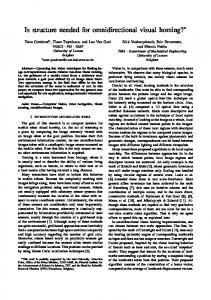
threshold or when the posterior probabilities indicate a noloop-closure event. In case of a no-loop-closure event, since the image does not belong to any of the places, we verify if it is addable to the current place node. Stricter conditions must be satisfied for an image to be added to the current node. The current node Nc is modeled as a hyper-sphere with center as the representative feature RNc (centroid of the member images’ VLAD features). A new feature can be added to the node only if the updated centroid is less than a distance of rn from all the member features as well as the new feature. The parameter rn is called node radius and ensures that all member features are tightly bound within this radius from the centroid. Finally, if the feature cannot be added to the current node a new node is formed with the feature itself being the centroid. The above discussed procedure might lead one to think of a possibility of using Mahalanobis distance (which is statistically stronger) in place of euclidean distance for similarity evaluation. However, Mahalanobis distance computation involves an inversion of covariance matrix of the features. An invertible covariance matrix can only be constructed if the sample set has at least 256 features (256 is the VLAD feature dimensionality). In other words, a node should have at least as many features as the feature dimensionality. Unfortunately the number of images represented per node is far less than 256 as will be shown in section V. B. Image Similarity Given a set of relevant nodes Nw a reference image set IR = {Ir1 , Ir2 , ...} is constructed by the union of relevant nodes’ member images. Image similarities are computed by combining two similarity measures namely the VLAD descriptor similarity and the spatial similarity. VLAD descriptor similarity is computed as the euclidean distance between the query image VLAD descriptor Dq and the reference image descriptor. The second similarity measure evaluates spatial similarity between two omnidirectional images (assumed to be unwrapped panoramas as the images in Figure 1). Let us consider two omnidirectional images acquired at approximately same location but with different heading directions ; and the robot is assumed to move in locally planar environments. Since the omnidirectional images have a circular field of view, distances between different objects in an image are well preserved even under a change in heading direction and a slight translation. In other words, the spatial structure of the objects(also applies to local image features) does not change with an in-place rotation of the camera. Hence if two images are from the same place, all objects in the first image should be shifted by the same amount to take their positions in the second image. A zero shift in object/feature coordinates indicates that the images are acquired in the same place and same heading direction, while a non-zero shift indicates same place with different heading. In case of a non match different objects will have different shifts. This situation is illustrated in Figure 1 from which, one can infer that the feature shifts
keypoints as a representative keypoint of all occurrences of the visual word. While adding shifts corresponding to the mean keypoints to the shift histogram, the corresponding bins are updated by the number of occurrences of the visual word. All the experimental results provided in this paper are generated by using this approximation. Weighted means of x and y shifts are computed using the shift histograms (lines 22-31). Weighted mean is used instead of regular mean to build robustness towards outliers. Then the distances of all shifts to the weighted mean is computed and organized in a distance histogram with L bins (lines 32-36). The final similarity score is computed using the histogram by assigning weights that are inversely proportional to the distance the bin corresponds to (lines 39, 40). This way, the first bin elements which contains all the shifts closest to the mean and get multiplied by the highest weight as a contribution to the similarity score. Similarly, the higher distance the bin corresponds to, the lower its contribution to the similarity. Note that the above discussed spatial similarity evaluation is only robust to minor translations and variable heading. However, it perfectly captures the definition of a loop closure.
(a) True Match
300
280
280
260
260
Shift in Y coordinates
Shift in Y coordinates
(b) False Match 300
240 220 200 180 160 140
220 200 180 160 140
120 100 200
C. Map Update
240
120
220
240
260
280
300
320
340
Shift in X co ordinates
360
380
400
100 200
220
240
260
280
300
320
340
360
380
400
Shift in X co ordinates
(c) True Match Feature (d) False Match Feature Shifts Shifts
Fig. 1: Feature Shift analysis of a true match and a false match. 1a shows features matched across a pair of images which are acquired in the same place. Matches are shown with blue lines. Shift in X and Y coordinates of a matched feature pair is demonstrated with a red dashed line. 1b shows illustrates a false match of a pair of images acquired at different places. 1c and 1d show the plots of matched feature shifts corresponding to the true and false match cases respectively.
of the true loop closure follow a converging pattern and those of the false loop closure look dispersed. The major hurdle here is to mathematically discriminate true matches from false matches using the shift values while being robust to the outliers. Algorithm 2 details the feature shift analysis. The first procedure shows structure of image similarity evaluation, which includes a call to the spatial similarity evaluation procedure. To compute spatial similarity, initially, the feature shifts are accumulated into histograms (lines 10-17). There can be problems in accommodating features which are shifted beyond the right border of the image start appearing on the left and vice versa. To tackle this problem, image width is used in order to measure shifts in x coordinates only in one direction. Another problem is in case of multiple instances of the same visual word in one or both images. For this we have an efficient clustering based solution. However, to keep things simple, an approximation is made by picking the mean of the
When the query image is similar to the current node or when a new node is to be formed, the query image is simply added to the corresponding node and the node centroid is updated. However in the third case an image similarity analysis has to be performed to compute likelihoods (Likelihood Evaluation procedure in Algorithm 2), which in turn are used to compute posterior probabilities of loop closure. The likelihoods obtained are plugged into equation 1 to get the posterior probability at each time step. A posterior probability greater than or equal to 0.9 is considered to be a loop closure. In such a case, the image It is added to the corresponding node only if the past m time-steps had loop closures with the node Ni or one of its neighbors. V. EXPERIMENTS Experimental results are presented on two datasets : the NewCollege dataset [7] and the Institut Pascal Dataset (IP dataset). NewCollege dataset is a popular laser and vision dataset from Oxford. Panoramas from the LadyBug camera are used for our experiments. The dataset also contains GPS readings but they are only partly stable and hence are not very useful for ground truth construction. Hence loop closure accuracies were determined through manual inspection. The second dataset (IP dataset) is our own multisensor containing two sequences: PAVIN and Cezeaux. The datasets constitute sensor readings from multiple sensors acquired using a VIPALAB platform. Platform and sensor details can be found on the website of the dataset 1 . From 1 The IP datasets website is: http://wwwlasmea.univbpclermont.fr/Personnel/Jonathan.Courbon/IPDS/ . Currently the omnidirectional images and the associated differential GPS readings are available for download and the remaining sensor data will be available from 1st November.
Sequence PAVIN (IP) Cezeaux (IP) NewCollege
Algorithm 2 Image Similarity Computation 1: procedure L IKELIHOOD E VALUATION(IR,Iq ) 2: likelihoods = [] 3: for each image i in IR do 4: di = Euclidean Distance(Di , Dq ) 5: ⊲ Di , Dq are VLAD descriptors. 6: si = Spatial Similarity(Zi , Zq , W, H, b) 7: ⊲ Zi , Zq are lists of quantized words of SURF features. 8: ⊲ W - Width of images, H- Height of images 9: ⊲ b- Bin width for shift histograms. 10: likelihoods(i) = di ∗ si 11: end forreturn likelihoods 12: end procedure 1: procedure S PATIAL S IMILARITY(Zi, Zq , W ,H,b) 2: M = Zi ∩ Zq ⊲ Accumulate feature matches. 3: n = size(M) ⊲ Number of matches. 4: num x bins = W/b 5: num y bins = W/b ⊲ Histogram of x-coordinate shifts. 6: HX = [num x bins] ⊲ Histogram of y-coordinate shifts. 7: HY = [num y bins] 8: shif ts = [] ⊲ Vector holding x & y shifts. 9: for each matched word wj in M do ⊲ Computes shifts for
#(Images) 8002 80913 7854
Trajectory 1.3 km 15.4 km 2.2 km
Velocity 2.3 m/sec 2.5 m/sec 1.0 m/sec
FPS 15 frames/sec 15 frames/sec 3 frames/sec
(a) Datasets Description Sequence PAVIN (IP) Cezeaux (IP) NewCollege
FPS 2 frames/sec 2 frames/sec 1.5 frame/sec
#(Images) 1144 11571 3977
(b) Data used for Experimentation. Parameter Name Bag of words vocabulary size for VLAD SURF descriptor size Full VLAD descriptor size PCA VLAD descriptor size kernel width for node similarity Node radius Node Similarity Threshold Bin width for shift histogram #(bins) for distances histogram Vocabulary size for spatial similarity Minimum supporting loop closures
Variable k l k∗l σ rn Tn b L m
Value 128 64 8192 256 0.84/1.08 0.7/0.9 0.3/0.4 10 10 32768 4
TABLE I: Parameters
matched words.
10: ki = get coordinates(Ii , wj ) 11: kq = get coordinates(Iq , wj ) 12: if (kq .x ≤ kr .x) then 13: δx = kr .x − kq .x 14: else 15: δx = (W − kq .x) + kr .x 16: δy = (kq .y − kr .y); 17: end if 18: HX.add(δx) 19: HY.add(δy) 20: shif ts.append(δx, δy) 21: end for 22: xmean = 0; ymean = 0 23: wtx = []; wty = [] 24: for each bin j in HX do 25: ⊲ Computes weights for mean computation. 26: 27: wtx(j) = num elements(HX(j)) n 28: end for 29: for each bin j in HY do (j)) 30: wty(j) = num elements(HY n 31: end for 32: xmean = W eighted M ean(HX, wtx) 33: ymean = W eighted M ean(HY, wty) 34: Hdists = [L] 35: for each shift s in shif ts do 36: d = Euclidean Distance((xmean , ymean ), s) 37: Hdists .add(d) 38: end for 39: similarity score = 0 40: for each bin index j in Hdists do 41: k = num elements(Hdists(j) 42: similarity score = similarity score + 21j ∗ k 43: ⊲ Final similarity score.. 44: end for 45: return similarity score 46: end procedure
this dataset we make use of the unwrapped omnidirectional images and the associated differential GPS readings (linearly interpolated when necessary for ground-truth generation). IP dataset is a bit challenging because of the low resolution of the images acquired with the omnidirectional camera. The datasets contain many images (refer to Table Ia) but only subsets are used in this paper. More precisely, only around two images per second are considered, resulting 3977 images for NC dataset, 1144 for PAVIN sequence and 11571 for Cezeaux sequence (refer to Table Ib). Loop closures are considered when the image location is closer than 2 meters. Our algorithm runs on a laptop computer equipped with an intel core i7 under linux. A. Parameters and Learning All the parameters used in our system are shown in table I. 64−dimensional Upright SURF (USURF-64) are used in all the places whenever local image features are needed. Training data is formed by selecting 25% of images from each sequence; SURF features extracted on all the training images are used in learning the bag of words vocabularies for VLAD computation and spatial similarity evaluation. These two vocabularies are learned using a single vocabulary tree - the first level of the tree contains 128 nodes and each of these nodes are again split with a branching factor of 4 for 4 levels having a total of 128 ∗ 44 = 32768 leaf nodes. Each SURF feature is quantized at two levels - one at the first level of the tree (forms a 128-word vocabulary) which is used for VLAD and the other at the leaf nodes (forms a 32768−word vocabulary) which is used for spatial similarity analysis. Full VLAD descriptors computed on all the training images are used to learn the PCA matrix P .
1 NewCollege Pavin Cezeaux
0.9
1 0.9
0.8 0.8
0.7 0.7
Precision
Precision
0.6 0.5 0.4
0.6 0.5 0.4
0.3 0.3
0.2 0.2
NewCollege PAVIN Cezeaux
0.1 0.1
0 0
0.2
0.4
0.6
0.8
1
0
Recall
0
0.1
0.2
0.3
0.4
0.5
0.6
0.7
0.8
0.9
1
Recall
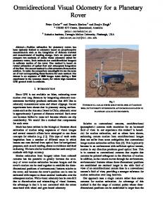
Fig. 2: Precision-Recall of Node Similarity Evaluation. rn 0.7 0.9 0.9
#(Nodes) 126 60 572
#(images)/node 31.5 19.06 20.22
(Traj.)/node 17.5 m 21.6 m 26.2 m
TABLE II: Node Statistics. #(Nodes) - Number of nodes of the map built on the sequence. #(images)/node - Average number of images represented by each node. (Traj.)/Node Average trajectory length represented by each node.
100 95
90
Precision
Sequence NewCollege PAVIN Cezeaux
(a) Precision-Recall Without Spatial Similarity
85
80
75
70 NewCollege Cezeaux Pavin
65
60 55
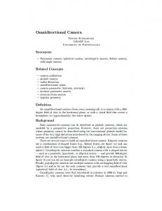
B. Node Similarity Analysis As mentioned earlier in the paper, node similarity analysis involves filtering the places in the map and selecting the most similar nodes. This process leads to good results only if it produces good recall rates even with bad precision. This means that the retrieved nodes should contain all the loop closure images which leads to high recall rates. However, since the nodes also contain many more images other than the true matches, the precision values can be far from 100%. This is evident from figure 2, which shows the precision-recall values obtained by varying the node similarity threshold rn . For best precision, node radius for PAVIN and Cezeaux sequences was set as rn = 0.9 and that of newcollege sequence as rn = 0.7. The kernel width for node similarity computation is chosen to be σ = 1.2 ∗ nr , so that it can give a slight cushion which accounts for noise in node similarity evaluation. Table II shows various node statistics of the maps built on the three sequences. It can be observed that the average number of images represented per node is between 20 and 30. As pointed out earlier this number is far less than 256 (VLAD descriptor length) to be useful for computing inverse of covariance matrix for computing Mahalanobis distance. C. Accuracy After the image similarity analysis, loop closure decision is taken. The precision and recall of these loop closures are shown in the Figure 3. Figure 3a illustrates the precisionrecall of the loop closure decisions computed without using the spatial similarity measure and only using the VLAD descriptor similarity. The curves are computed by varying the similarity threshold Ts which controls which reference nodes (and therefore reference images) are considered for image similarity analysis. We can see that 100% precision is only possible till 35% recall for the newcollege sequence, 24% for
60
65
70
75
80
85
90
95
100
Recall
(b) Precision-Recall With Spatial Similarity
Fig. 3: Precision-Recall graphs on the reference datasets.
the PAVIN sequence. Also 100% precision was never reached on the Cezeaux sequence. The reason is the low resolution images and the significant variation in illumination. Figure 3a illustrates the improved precision-recalls obtained by using the spatial constraint, where the recall of newcollege sequence is extended by 41% to a total of 76% and that of PAVIN has seen an improvement by 58% reaching a total of 82% at 100% precision. Spatial constraints also helped the Cezeaux sequence which achieved a recall of 55% with 100% precision. Hence the advantage of spatial constraints in increasing precision is demonstrated. It should be noted that no geometric verification has been applied to obtain the results. Figure 4 shows an example false loop closure which has been pointed out by using using spatial constraints. Loop closure maps over PAVIN, Cezeaux and NewCollege sequences are shown in and a loop closure scenario each are showed in Figure 5. We have used our datasets and training data to compare our accuracies with the FABMAP 2.0 2 algorithm as the authors recently opened ther code to the public. We have used the default parameters of the algorithm [1]. A vocabulary of zise equal to that of ours is used but on USURF-128 features (128 dimensional) as opposed to USURF-64 used by us. Precision and recall were analysed by varying the feature extraction threshold (varying the number of features per image) and the loop closure posterior threshold. Full Precision is obtained till 45% recall on PAVIN, 43% recall on 2 http://www.robots.ox.ac.uk/ mobile/wikisite/ pmwiki/pmwiki.php?n=Software.FABMAP
(a)
Fig. 4: A perceptual aliasing situation from NewCollege dataset eliminated using spatial constraints in image matching.
(a) PAVIN
NewCollege and 19% recall on Cezeaux datsets. RANSAC based epipolar geometry verification was not used after posterior computation with FABMAP. This serves as an evidence to prove that our technique is much more robust than FABMAP as our loop closure recall is rate is almost double than that of FABMAP on all three datasets. Also, all our loop closure accuracy results were reported without any additional geometrical checking. D. Computational Time Real-time operation is one of the vital elements of loop closure. There are five major modules in our algorithm: local feature extraction(SURF), local feature quantization, VLAD Extraction, Node similarity analysis and image similarity analysis. Map built on Cezeaux sequence is used in computational time analysis since it is the longest sequence of the three. SURF feature extraction takes 120 milliseconds on average and this is the most time consuming of the five modules. Feature quantization, VLAD extraction and node similarity analysis are performed within a few milliseconds as can be seen in Figure 6a. Figure 6b shows the image similarity analysis time along with the per frame processing time without local feature extraction. We can see that the per-frame processing time (excluding feature extraction) just reaches 40 milliseconds at maximum with 11571 images in the map. Almost 70% of the computation time is taken up by the local feature extraction. Including feature extraction, it takes a maximum of around 160 milliseconds per frame providing the capability of processing at least 5 frames per second. Such fast runtimes can even facilitate online map building (building the map during acquisition) on the datasets considered. VI. CONCLUSION A hierarchical mapping model is proposed which organizes images into places and represents them as nodes. Loop closure is hierarchically performed using VLAD descriptors
(b) CEZEAUX
(c) NewCollege
Fig. 5: Dataset sequence trajectories are plotted in red with regions were loop closures were detected are shown in green.
Computation Time (in seconds)
Local Feature Quantization 0.01 VLAD Extraction 0.009
Node Similarity Analysis
0.008 0.007 0.006 0.005 0.004 0.003 0.002 0.001 0 0
2000
4000
6000
8000
10000
Image ID
Computation Time (in seconds)
(a) Image similarity Analysis Total processing time per frame
0.05
0.04
0.03
0.02
0.01
0 0
2000
4000
6000 Image ID
8000
10000
(b)
Fig. 6: Runtimes for various modules of the loop closure algorithm. Figure 6a plots runtimes for the feature quantization time, VLAD extraction time and Node similarity analysis. Figure 6b shows the runtimes of image similarity analysis and the total time taken to process each image frame.
and a spatial similarity measure for omnidirectional images is introduced to achieve higher precision. Experimental results show the sparsity, accuracy and computational time efficiency achieved by using our algorithm. Good recall rates were seen on the datasets even without performing a geometric consistency check. Due to restricted space, it was not possible to analyse the effect of parameters other than the ones discussed. Realtime operability was also shown to be possible with more than 10000 images in the map. A fast C++ implementation of our algorithm will be made publicly available soon. The model proposed can be improved by bypassing the need to perform a hierarchical similarity analysis. It makes more sense to perform loop closure or localize at the place/node level itself instead of examining images. This can be possible if we enable the system to directly apply the spatial similarity analysis on the place/node level. The direction of our future work leads towards this goal along with a robust probabilistic similarity evaluation model. R EFERENCES [1] M. Cummins and P. Newman, “FAB-MAP: Probabilistic localization and mapping in the space of appearance,” The International Journal of Robotics Research, vol. 27(6), pp. 647–665, 2008. [2] ——, “Highly scalable appearance-only slam : Fab-map 2.0,” in Robotics Science and Systems, Seattle, USA, 2009. [3] A. Angeli, D. Filliat, S. Doncieux, and J.-A. Meyer, “A fast and incremental method for loop-closure detection using bags of visual words,” IEEE Transactions On Robotics, Special Issue on Visual SLAM, vol. 24(5), pp. 1027–1037, Oct. 2008.
[4] D. Galvez-Lopez and J. Tardos, “Real-time loop detection with bags of binary words,” in IEEE/RSJ International Conference on Intelligent Robots and Systems (IROS), San Francisco, CA, USA, Sep. 2011, pp. 51–58. [5] H. J´egou, M. Douze, C. Schmid, and P. P´erez, “Aggregating local descriptors into a compact image representation,” in IEEE Conference on Computer Vision & Pattern Recognition, San Francisco, USA, 2010, pp. 3304–3311. [6] H. Bay, T. Tuytelaars, and L. V. Gool, “SURF: Speeded up robust features,” Computer Vision and Image Understanding (CVIU), vol. 110, no. 3, pp. 346–359, 2008. [7] M. Smith, I. Baldwin, W. Churchill, R. Paul, and P. Newman, “The new college vision and laser data set,” The International Journal of Robotics Research, vol. 28(5), pp. 595–599, 2009. [8] N. Nourani-Vatani and C. Pradalier, “Scene change detection for vision-based topological mapping and localization,” in IEEE/RSJ International Conference on Intelligent Robotics and Systems (IROS), Taipei, Taiwan, Oct. 2010, pp. 3792–3797. [9] M.-L. Wang and H.-Y. Lin, “A hull census transform for scene change detection and recognition towards topological map building,” in IEEE/RSJ International Conference on Intelligent Robotics and Systems (IROS), Taipei, Taiwan, Oct. 2010, pp. 548–553. [10] A. Ranganathan, “Pliss: Detecting and labeling places using online change-point detection,” in Robotics: Science and Systems, Zaragoza, Spain, Jun. 2010. [11] Z. Zivkovic, O. Booij, and B. Krose, “From images to rooms,” Robotics and Autonomous Systems, vol. 55(5), pp. 411–418, 2007. [12] H. Korrapati, J. Courbon, Y. Mezouar, and P. Martinet, “Image sequence partitioning for outdoor mapping,” in IEEE International Conference on Robotics and Automation, ICRA’12, St. Paul, MN, USA, 2012, pp. 13–18. [13] C. Murillo, P. Campos, J. Kosecka, and J. Guerrero, “Gist vocabularies in omnidirectional-images for appearance based mapping and localization,” in 10th OMNIVIS, Zaragoza, Spain, Jun. 2010, pp. 1–9. [14] J. Kosecka, F. Li, and X. Yang, “Global localization and relative positioning based on scale-invariant keypoints,” Robotics and Autonomous Systems, vol. 52, no. 1, pp. 27–38, 2005. [15] C. Valgren and A. Lilienthal, “Incremental spectral clustering and seasons: Appearance-based localization in outdoor environments,” in IEEE International Conference on Robotics and Automation (ICRA), May 2008, pp. 1856–1861. [16] A. Oliva and A. Torralba, “Modeling the shape of the scene: a holistic representation of the spatial envelope,” International Journal of Computer Vision, vol. 42(3), pp. 145–175, May–June 2001. [17] F. Fraundorfer, C. Engels, and D. N´ıster, “Topological mapping, localization and navigation using image collections,” in IEEE/RSJ International Conference on Intelligent Robots and Systems, IROS’07, San Diego, USA, Oct. 2007, pp. 3872–3877. [18] R. Paul and P. Newman, “Fab-map 3d: Topological mapping with spatial and visual appearance,” in IEEE International Conference on Robotics and Automation (ICRA), Anchorage, Alaska, USA, May 2010, pp. 2649–2656. [19] D. Lowe, “Distinctive image features from scale-invariant keypoints,” International Journal of Computer Vision, vol. 60, no. 2, pp. 91–110, Nov. 2004. [Online]. Available: http://www.cs.ubc.ca/˜ lowe/keypoints/ [20] D. Nist´er and H. Stew´enius, “Scalable Recognition with a Vocabulary Tree,” in IEEE Conference on Computer Vision and Pattern Recognition (CVPR), vol. 2, New York City, USA, Jun. 2006, pp. 2161–2168. [21] J. Philbin, O. Chum, M. Isard, J. Sivic, and A. Zisserman, “Lost in quantization: Improving particular object retrieval in large scale image databases,” in IEEE Conference on Computer Vision and Pattern Recognition (CVPR), Jun. 2008, pp. 1–8. [22] S. Thrun, W. Burgard, and D. Fox, Probabilistic Robotics (Intelligent Robotics and Autonomous Agents series. The MIT Press, 2005.