Omnidirectional Sparse Visual Path Following with Occlusion-Robust

Omnidirectional Sparse Visual Path Following with Occlusion-Robust Feature Tracking Toon Goedem´e, Tinne Tuytelaars and Luc Van Gool

Gerolf Vanacker and Marnix Nuttin

VISICS - PSI - ESAT University of Leuven, Belgium {tgoedeme, tuytelaa, vangool}@esat.kuleuven.be

PMA - Department of Mechanical Engineering University of Leuven, Belgium {gerolf.vanacker, marnix.nuttin}@mech.kuleuven.be

Abstract— Omnidirectional vision sensors are very attractive for autonomous robots because they offer a rich source of environment information. The main challenge in using these for mobile robots is managing this wealth of information. A relatively recent approach is the use of fast wide baseline local features, which we developed and use in the novel sparse visual path following method described in this paper. These local features have the great advantage that they can be recognized even if the viewpoint differs significantly. This opens the door to a memory efficient description of a path by sparsely sampling it with images. We propose a method for reexecution of these paths by a series of visual homing operations. Motion estimation is done by simultaneously tracking the set of features, with recovery of lost features by backprojecting them from a local sparse 3D feature map. This yields a navigation method with unique properties: it is accurate, robust, fast, and without odometry error build-up.

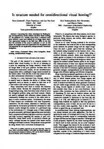
I. I NTRODUCTION In the broader scope of our research on vision-only robot navigation in natural and complex environments, this paper focuses on the algorithm we developed for sparse visual path following. In a previous step, a topological environment map is automatically built [1], [2]. This map represents the environment as a graph with as nodes omnidirectional images, each taken at a different place and as edges direct transversable connections between places. This paper presents a method for the re-execution of a path that is defined as a sequence of connected images. Fig. 1 illustrates this. The most obvious approach to achieve this is a series of visual homing operations. First, the robot is steered towards the place where the first of the path images is taken. From there, the next path image is aimed at, and so forth. Each of these elementary visual homing operations consists of steering a mobile robot from an arbitrary place in the neighborhood towards a place that is defined by an image taken there. In our approach, we work with path images that are taken relatively far from each other (’sparse’). That greatly diminishes the required memory space to describe a certain path. The application we envision for our method is a realtime automatic wheelchair [1] for indoor and outdoor use. During a training phase, all places are visited while recording omnidirectional images. Off-line, automatically a topological map is built from these sparse images, wherein nodes are

Fig. 1. Top: example of a topological map. Bottom: a sparse visual path, described by images 3 → 4 → 5 → 9 → 10 → 11.

crossroads and edges are paths, each path characterized by a sequence of images (e.g. fig. 1). When the patient in the wheelchair communicates a certain goal place to drive to, the wheelchair first localizes itself in the topological map (using a Bayesian localization scheme described in [2]), after which the path towards that goal is translated in a sequence of map images. This paper describes the way the wheelchair is steered along this sparse visual path. The remainder of this paper is organized as follows. Section II situates this paper between related work. In section III, an overview of the proposed algorithm is presented. The main two phases of each visual homing step of this algorithm are described in sections IV and V. Section VI details the experiments we have performed and section VII draws a conclusion. II. R ELATED WORK The essence of our method is a new approach to visual homing. Homing is a term borrowed from biology, where it is usually used to describe the ability of various living organisms, such as insects, to return to their nest or to a food source after having traveled a long distance. Many researchers have tried to imitate this behavior in mobile robots. Because of the complexity that working with images brings along, there have been many efforts to solve the navigation problem using non-visual sensors [3]. Vision is, in comparison with other sensors, much more informative.

We observe that many biological species, in particular flying animals, use mainly their visual sensors for localization and homing. Moreover, we see that the majority of insects and arthropods benefit from a wide field of view, which sustains our omnidirectional camera choice. A. Bearing-only visual homing Cartwright and Collett [4] proposed the so-called ’snapshot’ model. They suggest that insects fix the locations of landmarks surrounding a position by storing a snapshot image of the landmarks taken from that position. Their proposed algorithm consists of the construction of a home vector, computed as the average of landmark displacement vectors. Franz et al. [5] analyzed the computational foundations of this method and derived its error and convergence properties. They conclude that every visual homing method based solely on bearing (azimuth) angles of landmarks, inevitably depends on basic assumptions such as equal landmark distances, isotropic landmark distribution or the availability of an external compass reference. For instance, the snapshot-based method developed by Argyros et al. [6] silently assumes an isotropic landmark distribution. Unfortunately, because none of these assumptions generally hold in our targeted application we search for an alternative approach. Moreover, these methods return no information about home distance, which is necessary information for a mobile robot to determine the appropriate speed and to be able to stop safely at the home position if needed. B. Visual landmarks Crucial in all visual homing methods is the selection of the landmarks, to find corresponding pixels between the present image and the target image. Techniques based on optical flow [5], [7], [8] are used for this, although they are only suitable for small-baseline egomotion estimation. Other authors use artificial landmarks, like LEDs [9] or 2D barcodes [10]. For many applications, like ours, the use of artificial landmarks is out of the question because of its serious practical disadvantages. That is why we propose to use natural landmarks, found using the technique of local region matching. Instead of looking at the image as a whole, local regions are defined around interest points in the images. The characterization of these local regions with descriptor vectors enables the regions to be compared across images. Because of the built-in invariance against photometric and geometric changes, correspondences can be found between images with different lighting and different viewpoints. Many researchers proposed algorithms for local region matching. The differences between approaches lie in the way in which interest points, local image regions, and descriptor vectors are extracted. An early example is the work of Schmid and Mohr [11], where geometric invariance was still under image rotations only. Lowe [12] extended these ideas to scaleinvariance. More general affine invariance has been achieved

in the work of Baumberg [13] and Mikolajczyk & Schmid [14], that uses an iterative scheme and the combination of multiple scales, and in the more direct, constructive methods of Tuytelaars & Van Gool [15], [16], and Matas et al. [17]. Although these methods are capable to find good correspondences, most of them are too slow for use in a mobile robot algorithm. That is why we spent efforts to speed this up, as explained in section IV-A. C. Mapless, sparse maps, dense maps Ego-motion calculation is part of the problem presented. Both methods based on dense 3D maps (e.g. [18], [19]) and map-less appearance-based methods (e.g. [20]) are proposed. Methods on sparse maps, like ours, are situated between these two extremes and combine the avantages of both. Davison [21], for instance, developed a single projective camera SLAM method which estimates the ego-motion of the camera by building sparse probabilistic 3D maps with natural features. D. Epipolar geometry For visual homing, the most obvious choice is working via epipolar geometry estimation (e.g. [16], [22]). Unfortunately, in many cases this problem is ill conditioned. A workaround for planar scenes is presented by Sag¨ue´ s [23], who opted for the estimation of homographies. Svoboda [24] proved that motion estimation with omnidirectional images is much better conditioned compared to perspective cameras. That is why we chose a method based on omnidirectional epipolar geometry. Other work in this field is the research of Mariottini et al. [25], who split the homing procedure in a rotation phase and a translation phase, which can not be used in our application because of the non-smooth robot motion. E. Previous work In previous work [26], we developed a non-calibrated omnidirectional homing method based on Extended Kalman Filters. Visual features are found by wide baseline matching, and tracked throughout the sequence with a KLT tracker. During tracking, the 2D position of each feature, and also the present and target robot positions, are iteratively computed by means of an EKF. Although our tests proved quite successfull, this method shows two main disadvantages. Firstly, during tracking, inevitably features are lost due to tracking errors and occlusions. This results in a decreasing accuracy or even totally wrong motion towards the end of a homing operation. Another disavantage is the sensitivity of the Kalman filter to deviations in the initial state and the motion model. Moreover, an important amount of data is not used, because only bearing data is used and only 2D, not 3D maps are built. Our new approach, presented in this paper, avoids these problems. Based on epipolar geometry calculations using a calibrated omnidirectional camera, 3D feature maps are

can be stopped at a position close to the position where the last path image was taken. IV. I NITIALIZATION PHASE From each position within the reach of a target image, a visual homing procedure can be started. Our approach first establishes wide baseline local feature correspondences. That information is used to compute the epipolar geometry, which enables us to construct a local map containing the feature world positions, and to compute the initial homing vector. A. Wide baseline feature correspondences

Fig. 2.

Flowchart of the proposed algorithm.

built. This enables backprojection of features in the image to recover features that are lost during tracking. Another advantage is that the motion is not restricted to a plane. III. A LGORITHM OVERVIEW The aim is for a mobile robot to re-execute a path that is defined by omnidirectional images taken sparsely, say 1 to 3 metres from each other in a typical indoor environment along that path. As sketched in fig. 1, following such a sparse visual path boils down to a succession of visual homing operations. One of the advantages of this approach is the fact that no position errors build up during navigation. Each time the movement is relative to a new image position and previously made mapping and localization errors become irrelevant. Fig. 2 offers an overview of the proposed method. Each of the visual homing operations is performed in two phases, an initialization phase and an iterated tracking phase. First, the image taken at the present pose is compared with the next path image (the target image). Local feature correspondences between these two images permit calculation of the epipolar geometry between these images. From that, the homing vector required to move from the present to the target location, and the 3D positions of the features are computed. This initialization phase is described in section IV. Then, the robot is put into motion in the direction of the homing vector and an image sequence is recorded. In each new incoming image the visual features are tracked. Robustness to tracking errors (caused by e.g. occlusions) is achieved by reprojecting lost features from their 3D positions back in the image. These tracking results enable the calculation of the present location and from that the homing vector towards which the robot is steered. The tracking phase is detailed in section V. When the (relative) distance to the target is small enough, the entire homing procedure is repeated with the next image on the sparse visual path as target. If the path ends, the robot

Although wide baseline local features are common in computer vision, only recently, a class of fast wide baseline local features have appeared. We use the combination of two different kinds of these features, namely a rotation reduced and color enhanced form of Lowe’s SIFT features [12], and the invariant column segments we developed [27]. 1) Rotation reduced and color enhanced SIFT: David Lowe presented the Scale Invariant Feature Transform [12], which finds interest points around local peaks in a series of difference-of-Gaussian (DoG) images. A dominant gradient orientation and scale factor define an image patch around each interest point so that a local image descriptor can be found as a histogram of the gradient directions of the normalized image patch around the interest point. SIFT features are invariant to rotation and scaling, and robust to other transformations. A reduced form of these SIFT features for use on mobile robots is proposed by Ledwich and Williams [28]. They used the fact that rotational invariance is not needed for a camera fixed on a mobile robot moving in a plane. Elimination of the rotational normalization and rotational part of the descriptor yields a somewhat less complex feature extraction and more robust feature matching performance. Because the original SIFT algorithm works on grayscale images, some mismatches occur at similar objects in different colors. That is why we propose an outlier filtering stage based on a color descriptor of the feature patch based on global color moments, introduced by Mindru et al. [29]. We chose three color descriptors: CRB , CRG and CGB , with R R XY dΩ dΩ R , (1) CXY = R X dΩ Y dΩ where X, Y ∈ {R, G, B}, i.e. the red, green, and blue color bands, centralized around their means. After matching, the correspondences with Euclidean distance between the color description vectors above a fixed threshold are discarded. Between the image pair in fig. 3 the original SIFT algorithm finds 13 correct matches. Using this rotation reduced and color enhanced algorithm, the matching threshold can be raised so that up to 25 correct matches are found without including erroneous ones. These numbers, although very dependent on the complexity of the scene, are typical.

Fig. 4. Fig. 3. A pair of 320 × 240 omnidirectional images, superimposed with color-coded corresponding column segments (radial lines) and SIFT features (circles with tail).

2) Invariant column segments: In earlier work [27], we developed wide baseline features which are specially suited for mobile robot navigation. Taking advantage of the movement constraints of a fixed camera on a robot moving in a plane (although [27] shows robustness to minor violations of this constraint), a very simple and fast algorithm can be carried out. The (dewarped) image is scanned columnwise and column segment features are defined between two local maxima of the image gradient. Each column segment is described by an 11-element vector containing geometrical, color and intensity information. Fig. 3 shows the matching results on a pair of omnidirectional images. As seen in these examples, the SIFT features and the column segments are complementary, which pleads for the combined use of the two. The computing time required to extract features in two 320 × 240 images and find correspondences between them is about 800 ms for the enhanced SIFT features and only 300 ms for the vertical column segments (on a 800 MHz laptop). Typically 30 to 50 correspondences are found. Because only the local features are used and not the very pixel data itself, a path is described very memory efficiently by solely the local feature data of the sparse path images. B. Epipolar geometry estimation Our single-viewpoint omnidirectional camera is composed of a hyperbolic mirror and a perspective camera. As imaging model, we use the model proposed by Svoboda and Pajdla [24] (which is less general, but less complicated than the one by Geyer and Daniilidis [30]). This enables the computation of the epipolar geometry based on 8 point correspondences. In [31], Svoboda describes a way to robustly estimate the essential matrix E, when there are outliers in the correspondence set. Their so-called generate-and-select algorithm is based on repeatedly solving an overdetermined system built from the correspondences that have a low outlierness and evaluating the quality measure of the resulting

Projection model for a pair of omnidirectional images.

essential matrix. Because our tests with this method did not yield satisfactory results, we implemented an alternative method based on the well-known Random Sample Consensus (RANSAC [32]) paradigm. The set-up is sketched in fig. 4. One visual feature with world coordinates X is projected via point u on the first mirror to point p in the image plane of the first camera. In the second camera, the mirror point is called v and the image plane point q. For each of the correspondences, the mirror points u and v can be computed as u = F (K −1 p)K −1 p + tC ,

(2)

with tC = [0, 0, −2e]T and F (x) =

b2 (ex1 + akxk) . b2 x21 − a2 x22 − a2 x23

(3)

In these equations K is the internal matrix of the camera, and a, b and √ e are the parameters of the hyperbolic mirror, with e = a2 + b2 . If E is the essential matrix, for all correspondences vT Eu = 0. This yields for each correspondence pair one linear equation in the coefficients of E = [eij ]. The essential matrix can be computed as the solution of the homogeneous system Ae = 0, (4) with e = [e11 , e12 , e13 , e21 , . . . , e33 ] and the rows of A equal to ai = [vi1 ui1 , vi1 ui2 , vi1u ui3 , . . . , vi3 ui3 ]. For each random sample of 8 correspondences, an E matrix can be calculated. This is repeatedly done and for each E matrix candidate the inliers are counted. A correspondence is regarded an inlier if the second image point q lies within a predefined distance from the epipolar ellipse, defined by the first image point q. This epipolar ellipse B with equation xT Bx = 0 is computed as " # 2 2 2 2 4 4 2 2 2 B=

−4t a e + r b rsb4 rtb2 (−2e2 + b2 )

rsb −4t2 a2 e2 + s2 b4 stb2 (−2e2 + b2 )

rtb (−2e + b ) stb2 (−2e2 + b2 ) t 2 b4

(5)

with [r, s, t] = Eu = E(F (K −1 p)K −1 p+ tC ). Fortunately, this ellipse becomes a circle when the motion is in one plane, so that the distance from a point to this shape is easy to compute. From the essential matrix E with the maximal number of inliers the motion between the cameras can be computed using the SVD based method proposed by Hartley [33]. If more than one E-matrix is found with the same maximum number of inliers, the one is chosen with the smallest quality measure qE = σ1 − σ2 , where σi is the ith singular value of the matrix E. C. Local feature map estimation In order to start up the succession of tracking iterations, an estimate of the local map must be made. In our approach the local feature map contains the 3D world positions of the visual features, centered at the starting position of the visual homing operation. These 3D positions are easily computed by triangulation. It may arouse suspicion that we only use two images, the first and the target image, for this triangulation. This has two reasons. Firstly, these two have the widest baseline and therefore triangulation is best conditioned. Our wide baseline matches between these two images are also more plentiful and less influenced by noise than the tracked features. V. T RACKING

PHASE

When estimates of the homing vector and local map are found, the robot is put into motion in the direction of that homing vector. We rely on a lower-level collision detection and obstacle avoidance algorithm to do this safely [34]. During this drive, images are taken giving information to update the location of the robot. When close enough to one target, the movement towards the next target image is started. This yields a smooth trajectory along a sparsely defined visual path. A. Feature tracking The corresponding features found between the first image and the target image in the previous step, also have to be found in the incoming images during driving. This can be done very reliably performing every time wide baseline matching with the first or target image, or both. Although recent methods are relatively fast (about 0.8s for a pair of 640 × 480 images, see [27]), this is still too time-consuming for a driving robot. Because the incoming images are part of a smooth continuous sequence, a better solution is tracking. In the image sequence, visual features move only a little from one image to the next, which enables to find the new feature position in a small search space. A widely used tracker is the KLT tracker of Kanade, Lucas, Shi, and Tomasi [35]. KLT starts by identifying interest points (corners), which then are tracked in a series of images. The

basic principle of KLT is that the definition of corners to be tracked is exactly the one that guarantees optimal tracking. A point is selected if the matrix  2  gx gx gy , (6) gx gy gy2 containing the partial derivatives gx and gy of the image intensity function over an N × N neighborhood, has large eigenvalues. Tracking is then based on a Newton-Raphson style minimization procedure using a purely translational model. This algorithm works surprisingly fast: we were able to track 100 feature points at 10 frames per second in 320 × 240 images on a 800 MHz laptop. Because the well trackable points are not necessarily coinciding with the center points of the wide baseline features to be tracked, the best trackable point in a small window around such a center point is selected. In the assumption of local planarity we can always find back the corresponding point in the target image via the relative reference system offered by the wide baseline feature. B. Recovering lost features The main advantage of working with this calibrated system is that we can recover features that were lost during tracking. This avoids the problem of losing all features by the end of the homing maneuver, a weakness of our previous approach [26]. In the initialization phase, all features are described by an intensity histogram, so that they can be recognized after being lost during tracking. Each time a feature is successfully tracked, this histogram is updated. When tracking, some features are lost due to temporal invisibility because of e.g. occlusion. Because our local map contains the 3D positions of each feature, and the last robot position in that map is known, we can reproject the 3D feature in the image. Svoboda shows that the world point XC (i.e. the point X expressed in the camera reference frame) is projected on point p in the image: p=

K (λXC − tC ), 2e

(7)

wherein λ is the largest solution of λ=

b2 (−e)XC 3 ± akXC k . − a2 XC 21 − a2 XC 22

b2 XC 23

(8)

Based on the histogram descriptor, all trackable features in a window around the reprojected point p are compared to the original feature. When the histogram distance is under a fixed threshold, the feature is found back and tracked further in the next steps.

C. Motion computation When in a new image the feature positions are computed by tracking or backprojection, the camera position (and thus the robot position) in the general coordinate system can be found based on these measurements. It is shown that the position of a camera can be computed when for three points the 3D positions and the image coordinates are known. This problem is know as the three point perspective pose estimation problem. An overview of the proposed algorithms to solve it is given by [36]. We chose the method of Grunert, and adapted it for our omnidirectional case. The required input data, unit vectors pointing from the center of perspectivity to the observed points, is easily computed by normalizing the corresponding mirror points v. Also in this part of the algorithm we use RANSAC to obtain a robust estimation of the camera position. Repeatedly the inliers belonging to the motion computed on a three-point sample are counted, and the motion with the greatest number of inliers is kept. D. Robot motion In subsection IV-B is explained how the position and orientation of the target can be extracted from the computed epipolar geometry. Together with the present pose results of the last subsection, a homing vector can easily be computed. This command is communicated to the locomotion subsystem. When the homing is towards the last image in a path, also the relative distance and the target orientation w.r.t. the present orientation is given, so that the locomotion subsystem can steer the robot to a halt at the desired position. This is needed for e.g. docking at a table. VI. E XPERIMENTAL

RESULTS

A path was defined by four omnidirectional images taken at places about 2 metres apart along the path. From a starting position in the neighborhood of the first image, the visual path following algorithm was executed. Typical results of one visual homing step of our algorithm are presented in fig. 7 and 8. We prepared a demo video about this experiment which is downloadable via http://www.esat.kuleuven.be/∼tgoedeme. A. Test platform We have implemented the proposed algorithm, using our modified wheelchair ”Sharioto”. It is a standard electric wheelchair that has been equipped with an omnidirectional vision sensor (consisting of a Sony firewire color camera and a hyperbolic mirror). The image processing is performed on a 1 GHz laptop. As additional sensors for obstacle detection, 16 ultrasound sensors and a Lidar are added. A second laptop with a 840 MHz processor reads these sensors, receives visual homing vector commands, computes the necessary manoeuvres, and drives the motors via a CAN-bus. More information can also be found in [37] and [34].

1

1

0.9

0.9

0.8

0.8

0.7

0.7

0.6

0.6

0.5

0.5

0.4

0.4

0.3

0.3

0.2

0.2

0.1 0

0.1

0

20

40

60

80

100

0

120

0

20

40

60

80

100

120

Fig. 5. Homing direction error [rad] (left), and home orientation error [rad] (right) w.r.t. distance [%]. The goal location lies at 100% 4

3.5

3

2.5

2

1.5

1

0.5

0

1

1.5

Fig. 6.

2

2.5

3

3.5

4

4.5

5

5.5

6

Homing vectors from 1-meter-grid positions.

B. Initialization phase During the initialization phase of one visual homing step, correspondences between the present and target images are found and the epipolar geometry is computed. This is shown in fig. 7. We tested thouroughly the accuracy of the homing vector computed from the epipolar geometry. Fig. VI-B plots the angle error of the homing direction and the home orientation for different distances between first and target position. We see that the error decreases with decreasing distance to the goal. However, when the baseline becomes too small, the error goes up again due to ill-conditioning. For an other experiment, we took images with the robot positioned at a grid with a cell size of one meter. The resulting home vectors towards one of these images (taken at (6,3)) are shown in fig. 6. This proves the fact that even if the images are situated more than 6 metres apart the algorithm works thanks to the use of wide baseline correspondences. C. Tracking phase We present a typical experiment in fig. 8. During the motion, the top of the camera system was tracked in a video sequence from a fixed camera. This video sequence, along with the homography computed from some images taken with reference positions, permits calculation of metrical robot ground truth data. Repeated similar experiments showed an average homing accuracy of 11 cm, with a standard deviation of 5 cm. D. Timing The algorithm runs surprisingly fast on the rather slow hardware we used: the initialization for a new target lasts only 958 ms, while afterwards every 387 ms a new homing vector is computed.

Fig. 7. Results of the initialization phase. Top row: target, bottom row: start. From left to right, the robot position, omnidirectional image, visual correspondences and epipolar geometry are shown.

VII. C ONCLUSION In this work, we developed a novel approach to visual path following as a series of visual homing operations on path images. Image correspondences are found using advanced fast wide baseline feature matching techniques, which can cope with big viewpoint differences. This permits the use of only a few path images, which leads to the concept of a memory efficient sparse visual path. Based on robustly estimated omnidirectional epipolar geometry a local 3D map of the environment is built, which holds only the feature world coordinates (a sparse 3D map). This enables the recovery of features which are lost during tracking by backprojecting them in the image. In this sense an occlusion-robust feature tracker is built. Our experiments show the feasibility and robustness of this approach. ACKNOWLEDGMENTS T.G. thanks Eric Demeester and Dirk Vahooydonck. This work is partially supported by the Inter-University Attraction Poles, Office of the Prime Minister (IUAP-AMS), the Institute for the Promotion of Innovation through Science and Technology in Flanders (IWT-Vlaanderen), and the Fund for Scientific Research Flanders (FWO-Vlaanderen, Belgium). R EFERENCES [1] T. Goedem´e, M. Nuttin, T. Tuytelaars, and L. Van Gool, ”Vision Based Intell. Wheelchair Control: the role of vision and inertial sensing in topological navigation,” J. of Robotic Systems, 21(2), pp. 85-94, 2004. [2] T. Goedem´e, M. Nuttin, T. Tuytelaars, and L. Van Gool, ”Markerless Computer Vision Based Localization using Automatically Generated Topological Maps,” European Navigation Conf., Rotterdam, 2004. [3] S. Thrun, ”Learning Metric-Topological Maps for Indoor Mobile Robot Navigation,” AI Journal, 99(1), pp 21-71, 1999. [4] B. Cartwright, T. Collett, ”Landmark Maps for Honeybees,” Biol. Cybernetics, 57, pp. 85-93, 1987. [5] M. Franz, B. Sch¨olkopf, H. Mallot, and H. B¨ulthoff, ”Where did I take that snapshot? Scene-based homing by image matching,” Biological Cybernetics, 79, pp. 191-202, 1998.

[6] A. Argyros, K. Bekris, and S. Orphanoudakis, ”Robot Homing based on Corner Tracking in a Sequence of Panoramic Images”, Computer Vision and Pattern Recognition, vol. 2, p. 3, Kauai, Hawaii, 2001. [7] J. Gluckman and S. Nayar, ”Ego-Motion and Omnidirectional Cameras,” Proceedings of ICCV, p. 999, Bombay, 1998. [8] R. Vassallo, J. Santos-Victor, H. Schneebeli, ”A General Approach for Egomotion Estimation with Omnidirectional Images,” OMNIVIS’02 Workshop on Omni-directional Vision, Copenhagen, 2002. [9] D. Aliaga, ”Accurate catadioptric calibration for real-time pose estimation in room-size environments,” in Proc. IEEE Int. Conf. Computer Vision (ICCV), Vancouver, pp. 127–134, 2001. [10] J. Rekimoto and Y. Ayatsuka, ”CyberCode: Designing Augmented Reality Environments with Visual Tags,” Proc. of DARE, 2000. [11] C. Schmid, R. Mohr, C. Bauckhage, ”Local Grey-value Invariants for Image Retrieval,” International Journal on Pattern Analysis an Machine Intelligence, Vol. 19, no. 5, pp. 872-877, 1997. [12] D. Lowe, ”Object Recognition from Local Scale-Invariant Features,” International Conference on Computer Vision, pp. 1150-1157, 1999. [13] A. Baumberg, ”Reliable feature matching across widely separated views,” CVPR, Hilton Head, South Carolina, pp. 774-781, 2000. [14] K. Mikolajczyk and C. Schmid, ”An affine invariant interest point detector,” ECCV, vol. 1, 128–142, 2002. [15] T. Tuytelaars and L. Van Gool, ”Wide baseline stereo based on local, affinely invariant regions,” BMVC, Bristol, UK, pp. 412-422, 2000. [16] T. Tuytelaars, L. Van Gool, L. D’haene, and R. Koch, ”Matching of Affinely Invariant Regions for Visual Servoing,” Intl. Conf. on Robotics and Automation, pp. 1601-1606, 1999. [17] J. Matas, O. Chum, M. Urban and T. Pajdla, ”Robust wide baseline stereo from maximally stable extremal regions,” British Machine Vision Conference, Cardiff, Wales, pp. 384-396, 2002. [18] D. Nist´er, O. Naroditsky, J. Bergen, ”Visual Odometry,” Conference on Computer Vision and Pattern Recognition, Washington, DC, 2004. [19] E. Royer, M. Lhuillier, M. Dhome, and T. Chateau, ”Towards an alternative GPS sensor in dense urban environment from visual memory,” 15th British Machine Vision Conference, London, 2004. [20] T. Mitchell and F. Labrosse, ”Visual Homing: a purely appearancebased approach,” proc. Towards Aut. Robotic Systems, Colchester, 2004. [21] A. Davison, ”Real-time simultaneous localisation and mapping with a single camera,” Intl. Conf. on Computer Vision, Nice, 2003. [22] R. Basri, E. Rivlin, and I. Shimshoni, ”Visual homing: Surfing on the epipoles,” in IEEE ICCV’98, pp. 863-869, Bombay, 1998. [23] C. Sag¨ue´ s, J. Guerrero, ”Visual correction for mobile robot homing,” Robotics and Autonomous Systems, Vol. 50, no. 1, pp 41-49, 2005. [24] T. Svoboda, T. Pajdla, and V. Hlav´acˇ , ”Motion Estimation Using Panoramic Cameras,” Conf. Intell. Veh., Stuttgart, pp. 335-340, 1998. [25] G. Mariottini, E. Alunno, J. Piazzi, and D. Prattichizzo, ”Epipole-Based Visual Servoing with Central Catadioptric Camera,” IEEE ICRA05, Barcelona, 2005.

Fig. 8. Three snapshots during the motion phase: in the beginning (left), half (center) and at the end (right) of the homing motion. The first row shows the external camera image with tracked robot position. The second row shows the computed world robot positions [cm]. The third row shows the color-coded feature tracks. The bottom row shows the sparse 3D feature map (encircled features are not lost). [26] T. Goedem´e, T. Tuytelaars, G. Vanacker, M. Nuttin and L. Van Gool, ”Feature Based Omnidirectional Sparse Visual Path Following,” IROS, Edmonton, 2005. [27] T. Goedem´e, T. Tuytelaars, and L. Van Gool, ”Fast Wide Baseline Matching with Constrained Camera Position,” Computer Vision and Pattern Recognition, Washington, DC, pp. 24-29, 2004. [28] L. Ledwich and S. Williams, ”Reduced SIFT Features For Image Retrieval and Indoor Localisation,” ACRA, Canberra, 2004. [29] F. Mindru, T. Moons, and L. Van Gool, ”Recognizing color patters irrespective of viewpoint and illumination,” CVPR, pp. 368-373, 1999. [30] C. Geyer and K. Daniilidis, ”Mirrors in motion: Epipolar geometry and motion estimation,” ICCV, p. 766, Nice, 2003. [31] T. Svoboda, ”Central Panoramic Cameras, Design, Geometry, Egomotion,” PhD Thesis, Czech Technical University. [32] M. Fischler, R. Bolles, ”Random Sample Consensus: A Paradigm for

Model Fitting with Applications to Image Analysis,” Comm. of the ACM, Vol 24, pp 381-395, 1981. [33] R. Hartley, ”Estimation of relative camera positions for uncalibrated cameras,” 2nd ECCV, pp. 579-587, 1992. [34] E. Demeester, M. Nuttin, D. Vanhooydonck, and H. Van Brussel, ”Fine Motion Planning for Shared Wheelchair Control: Requirements and Preliminary Experiments,” ICRA, Coimbra, pp. 1278-1283, 2003. [35] J. Shi and C. Tomasi, ”Good Features to Track,” Computer Vision and Pattern Recognition, Seattle, pp. 593-600, 1994. [36] R. Haralick, C. Lee, K. Ottenberg, and M. N¨olle, ”Review and analysis of Solutions of the Three Point Perspective Pose Estimation Problem,” International Journal of Computer Vision, 13, 3, pp. 331-356, 1994. [37] M. Nuttin, E. Demeester, D. Vanhooydonck, and H. Van Brussel, ”Shared autonomy for wheelchair control: Attempts to assess the user’s autonomy,” in Autonome Mobile Systeme, pp. 127-133, 2001.