High-Accuracy Object Recognition with a New ... - CiteSeerX

High-Accuracy Object Recognition with a New Convolutional Net Architecture and Learning Algorithm Kevin Jarrett, Marc’Aurelio Ranzato, Koray Kavukcuoglu, Yann LeCun The Courant Institute of Mathematical Sciences New York University Purely supervised Convolutional Networks yield excellent accuracy on image recognition tasks when data is plentiful [1]. But until now, they have not produced state-of-the-art accuracy on object recognition benchmarks for which few labeled samples per category are available. For example, on the popular Caltech-101 dataset with 30 samples for each of the 101 categories, methods that use hand-designed features, such as SIFT and Geometric Blur combined with a kernel classifier, achieve accuracies of 66.2% [5], and 64.6% [6]. By contrast, a purely supervised convolutional network with standard sigmoid non-linearities yields only 26%. This abstract describes a modified ConvNet architecture with a new unsupervised/supervised training procedure that can reach 67.2% accuracy on Caltech-101. This work explores several architectural designs and training methods and studies their effect on the accuracy for object recognition. The convolutional network under consideration takes a 143x143 grayscale image as input. The preprocessing includes removing mean and performing a local contrast normalization (dividing each pixel by the standard deviation of its neighbors). The first stage has 64 filters of size 9x9, followed by a subsampling layer with 5x5 stride, and 10x10 averaging window. The second stage has 256 feature map, each with 16 filters connected to a random subset of first-layer feature maps. The subsampling layer has a stride of 4x4 and a 6x6 averaging window. Hence, the input to the last layer has 256 feature maps of size 4x4 (4096 dimensions). Figure 1 shows the outline of a convolutional net, and figure 2 shows the best sequence of transformations at each stage of the network. The results are shown in table . The most surprising result is that simply adding an absolute value after the hyperbolic tangent (tanh) non-linearity practically doubles the recognition rate from 26% to 58% with purely supervised training. We conjecture that the advantage of a rectifying non-linearity is to remove redundant information (the polarity of features), and at the same time, to avoids cancellations of neighboring opposite filter responses in the subsampling layers. Adding a local contrast normalization step after each feature extraction layer [4] further improves the accuracy to 60%. The second interesting result is that pre-training each stage one after the other using a new unsupervised method, and adjusting the resulting network using supervised gradient descent bumps up the accuracy to 67.2%. The procedure is reminiscent of several recent proposal for “deep learning” [2, 3]. Our layer-wise unsupervised training method is called Predictive Sparse Decomposition (PSD). It consist in learning an overcomplete set of basis functions from which 1

Id Accuracy (%) Protocol Machine Traditional ConvNet Architecture 1 26.0% RR Tanh, 64 features 2 30.0% AA Tanh, CNorm, 64 features With Absolute Value Non-Linearity 3 58.0% RR Abs, 64 features Abs and Contrast Normalization 4 60.0% RR Abs, CNorm, 64 features 5 62.0% AR Abs, CNorm, 64 features 6 62.9% PP Abs, CNorm, 64 features 7 63.0% PA Abs, CNorm, 64 features 8 67.2% AA Abs, CNorm, 64 features Smaller net with Abs and CNorm 9 59.8% PP Abs, CNorm, 16 features 10 65.2% AA Abs, CNorm, 16 features Table 1: Average recognition rate on Caltech-101. The training procedure are as follows. Each letter in the Training column indicates the training method used for each of the two feature extraction stages in the ConvNet (the last stage is always trained in supervised mode). R indicates a purely supervised learning from a random initial condition; P indicates unsupervised pre-training with no supervised adjustmentl; A indicates unsupervised pre-training with supervised adjustment. The traditional ConvNet architecture uses a hyperbolic tangent non linearity (tanh) at each layer. When trained in purely supervised mode from random initial weights, the traditional ConvNet yields only 26% (line 1), but reaches 58% when the tanh is replaced by an absolute value (line 3), and reaches 60.0% when a local contrast normalization step is added after each stage (line 4). Using unsupervised pre-training followed by supervised refinment (line 8) the accuracy reaches 67.2%. any input patch can be reconstructed under an L1 penalty on the coefficients. Normally, the exact set of coefficients for a given input patch must be obtained through a rather expensive energy minimization process. The crucial idea of PSD is to circumvent this step by training a feed-forward “encoder” that can predict the sparse solution for any input patch. This feedforward encoder allows a fast computation of feature vectors [7]. If the feature extraction stages are kept fixed after the unsupervised pre-training (only the last layer is trained supervised), the accuracy goes down to 62.9% (line 6 in the table). Hence, unsupervised pre-training helps considerably, but only when supervised refinement is performed after the pre-training phase. It seems that the features produced by the unsupervised training produce a good starting point for supervised training, but are not sufficiently class specific to provide good accuracy without supervision. Reducing the number of feature maps of the first layer to 16 instead of 64 lowers the accuracy by a mere 2% to 65.2%. This opens the door to real-time object recognizers. We will also give results of this new convolutional net on other datasets, such as MNIST and the Graz object dataset.

2

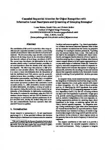
Figure 1: Architecture of a convolutional net. Each feature extraction stage is described in fig. 2. In this example, there are two feature extraction stages followed by a multinomial logistic regression classifier predicting the object class of the input image.

Figure 2: Operations performed by a single stage of feature extraction of a convolutional net. First the input is convolved with a set of trainable filters. Second, it is non-linearly transformed by a tanh non-linearity followed by some rectification (e.g., an absolute value). Then, it is contrast normalized and spatially down-sampled.

References [1] Y. LeCun, L. Bottou, Y. Bengio, P. Haffner, Gradient-Based Learning Applied to Document Recognition, IEEE 86(11) 1998. [2] G.E. Hinton and R.R. Salakhutdinov, Reducing the dimensionality of data with neural networks. Science, 313(5786) 2006. [3] M. Ranzato, F.J. Huang, Y. Boureau and Y. LeCun, Unsupervised Learning of Invariant Feature Hierarchies with Applications to Object Recognition. CVPR 2007. [4] M.N. Pinto, D.D. Cox, J.J. DiCarlo, Why is Real-World Visual Object Recognition Hard?. 4(1) PLoS 2008. [5] S. Lazebnik, C. Schmid, J. Ponce, Beyond Bags of Features: Spatial Pyramid Matching for Recognizing Natural Scene Categories. CVPR 2006 [6] H. Zhang, A.C. Berg, M. Maire, J. Malik, SVM-KNN: Discriminative Nearest Neighbor Classification for Visual Category Recognition. CVPR 2006 [7] K. Kavukcuoglu, M.’A. Ranzato, Y LeCun, Fast Inference in Sparse Coding Algorithms with Applications to Object Recognition, Tech Report CBLL-TR-2008-12-01, http://yann.lecun.com/exdb/publis/index.html#koray-psd-08 .

3