High-level parallel computing language Jianfeng Zhoua , Yang Yanga and Yan Sub a Center b National
for Astrophysics, Tsinghua University, Beijing 100084, China; Astronomical Observatories, Chinese Academy of Sciences, Chaoyang District, Datun Road 20A, Beijing 100012, China ABSTRACT
High-level Parallel Computing language (HPCL) combines the high performance of Clusters and the easy-to-use property of high-level language Octave. A HPCL program will run concurrently in a set of virtual machines (VMs). Therefore, HPCL programs are machine independent. HPCL keeps the elegant of the current high-level languages. It only needs one additional operator @ to transfer data and commands among the VMs. HPCL is also compatible to the conventional high-level language. Any sequential high-level Octave programs can be run properly in HPCL environment without modification. The realization of HPCL is briefly introduced in this report, including the main system components, execution strategy and message transfer protocol. Keywords: High-level, Parallel Language, Octave
1. INTRODUCTION The performance of CPU is increasing rapidly according Moore’s law, i.e. its speed will be doubled after about 18 months. The other properties, such as the size of RAM and hard disk have similar increment law. It’s price, however, is gradually decreasing. The high performance and low price make Cluster, a set of computer which are connected by high speed network, a cost effective and widely used supercomputer. In order to solve time consuming problem in a Cluster, we need to write parallel computing programs. There are several parallel languages or tools. For example MPI,1 PVM,2 CC++,3 ORCA,4 JADE5 etc.. These languages, however, are mainly depend on low level languages, such as C or FORTRAN. They have some disadvantages. Firstly, they are inefficient for programming. A small task may needs hundreds of lines of codes. Secondly, sequential programs can’t be run directly in parallel way. The original codes need to be modified or even rewritten for parallel execution. Thirdly, such languages are difficult to be mastered. So, most scientists wouldn’t like to learn it. Compare to low-level languages, high-level computing languages, such as IDL, Matlab, Octave 6 etc., have some notable features. They are very efficient for programming. Scientists and engineers probably only need tens of line of codes to realize a new idea. Also, most of the high-level language programs can be executed as fast as those C or Fortran programs. Finally, high-level languages usually provide very powerful data visualization interface. All these features made high-level languages the most popular programming languages for scientists and engineers. At present, most high-level languages can’t be directly used to write parallel programs. The main objective of our consideration is to expand the definition of high-level language, so that it can be used for writing parallel programs in an easy and natural way. The expanded language is called High-level Parallel Computing Language (HPCL). We use Octave, which is an opensource Matlab-compatible high-level language, as the basis of HPCL. Therefore, it will save us a lot of time to develop usable tools for running HPCL. In this report, the basic concept of HPCL will be introduced in section 2. In section 3, a brief approach of realization will be described. Send correspondence to Jianfeng Zhou. Jianfeng Zhou: E-mail:
[email protected], Telephone: +86 10 6279 2127
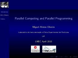
Figure 1. The structure of a 4-VM HPCL system. There are one client and three servers.
2. CONCEPT DESIGN 2.1. Structure The running environment of HPCL consists of a list of Virtual Machines (VM). Each VM is actually an independent Octave process, has its own command sets, and local variables. These VMs are connected each other through TCP/IP sockets. So they can exchange data as well as commands each other. An N-VM HPCL environment is composed of 1 client and N-1 servers, as displayed in Fig. 1. The master program usually is running in a client VM. It will dispatch data and command (messages) to server VMs and collect the results. For the convenient of programming, each VM is denoted by a nonnegative integer which is called VM index. Zero is assigned to client, and 1, 2, ..., N-1 are assigned to N-1 servers respectively. Each VM keeps a list where all VM indexes and their corresponding sock numbers are saved. Therefore, VMs know how to send data and commands to correct places.
2.2. Operator @ To enable a programming language with parallel computing ability. A conventional way is to add some message passing functions, such as send() and recv(). Here, we choose another way. We try to expand the definition of high-level language, so that it can naturally deal with parallel computing problems. Only one extra operator is needed to realize parallel or distributed computing for HPCL. For traditional accustomed consideration, such operator is denoted by @. Operator @ is used to indicate where are the data and where to send the commands. For example: A@vm1 means variable A is in VM1; ”B = M ∗ M ”@vm2 means the command B = M ∗ M should be sent to VM2 and executed there. Here, vm1 and vm2 are both nonnegative integers. Programs or expressions without operator @ mean they will be executed in local VM. Therefore, any sequential Octave (or Matlab) programs will run properly in HPCL environment.
2.3. Operation Rules of @ To write a correct HPCL program, the following rules should be considered and followed.
2.3.1. Rule 1 All data and variables are calculated by local functions or operators. As mentioned in section 2.1, each VM has its independent computing environment. It has build-in functions, and knows where to load external functions. The calculations concerning the data in a VM will only use the functions in the same VM. For example, the commands in VM vm1 A@vm1 + B@vm1 sin(B@vm1)
(1) (2)
A+B sin(B)
(3) (4)
will be translated to
and sent to VM with index vm1 and executed there. 2.3.2. Rule 2 When data in the left side of an operator and those in the right side of an operator are in different VMs, the latter data must be copied or transfered to the former VM, and then executes the operation. Here are some examples : A
=
B@vm1
(5)
A A
+ ∗
B@vm2 B@vm2
(6) (7)
A
.
B@vm2.
(8)
The first line of commands mean one temporary copy of variable B in vm1 will be generated in local VM, and will be assigned to variable A. Line 2, 3, 4 indicate that B in vm2 will be copied to local VM, and then added or multiplied with A. 2.3.3. Rule 3 In a same priority level, the operation will be run in the VM where the first variable locates. For example, A + B@vm1 + C@vm2 will be computed in local VM, and the copies of B in vm1 and C in vm2 will be transfered to the local VM. A@vm0 + B@vm1 + C@vm2 For this expression, the local VM will first translate it into A + B@vm1 + C@vm2, then the new expression will be sent to VM vm0. The parser in vm0 will calculate this expression, and return the result back to the local VM finally. A@vm0 ∗ B@vm1 ∗ C@vm2 The execution of this expression is the same as that in above example.
A@vm0 + (B@vm1 + C@vm2) When the parser in local VM meets this expression, it will translate the expression into A + (B@vm1 + C@vm2), and send it to VM vm0. Again, the parser in vm0 will translate the subexpression B@vm1 + C@vm2 into B + C@vm2, and send it to VM vm1. The subexpression will be calculated in vm1, and the results will be returned to vm0. The whole expression will be computed in vm0, and its result will be transfered back to the local VM. A@vm0 + B@vm1 ∗ C@vm2 The execution of this expression is similar to that in above example. 2.3.4. Rule 4 Functions will be executed in a VM where their first parameter locates. For example, cos(A@vm0) will be run in VM vm0. Add(B@vm1, C@vm2) will be run in VM vm1, and C@vm2 will be copied into this VM. 2.3.5. Rule 5 ’commands’@vmi means the commands will be sent to VM vmi and executed there, return the results. ”commands”@vmi means the commands will be sent to VM vmi and executed there, but no results return. For instance, 0
A ∗ B 0 @vm1
sends command A ∗ B to vm1 and returns the results. ”spectrum = f f t(timeseries)”@vm1 calculates the spectrum of the time series in vm1, but doesn’t return the results.
2.4. An example of HPCL program The example program below demonstrates how to calculate the power spectrum of large data. The program will be executed in client (VM 0) firstly. lc = load lc.txt ; #Load light curve data, altogether 10*N. for i = 1 : 10 lc@i = lc( (i-1)*N+1, i*N ) ; #Extract part of data, and dispatch them to 10 VMs. " sp = fft( lc ); "@i ; #Calculate the spectrum of the light curve data #in each VM. end for i = 1 : 10 sp += sp@i ; #Collect and combine the spectrum. end
Message Transfer Channel
Spawn VMs
VM3
VM1
Spawn VMs
VM Manager 2
VM Manager 1
VM4
VM2
Request VMs
Request VMs VM0 : Client
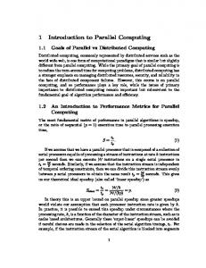
Figure 2. The system components and their relationships of HPCL. According to the requirement a HPCL program, the client will send requests to VM Managers to construct VMs (servers). The data and commands transferring channels will be built between all VMs. After the program finished, the VM Managers will delete all VM servers.
An important feature for parallel programming of HPCL is we should always dispatch data and commands first, then collect the results. In above example, the data collection codes sp+ = sp@i are in an independent circulation. If data dispatch and collection commands are in a same circulation, then after sending the first part of data, the parser will wait till the results is ready in VM 1. This will greatly delay the dispatch of other data and commands.
3. REALIZATION 3.1. System Components The system components of HPCL include a set of VMs, which are divide into one client and several servers. VM manager is also an important component, which controls the construction/destruction of VMs under the requests of client. The relationships between these components are shown in Fig. 2. 3.1.1. Octave GNU Octave is a high-level language, primarily intended for numerical computations. It provides a convenient command line interface for solving linear and nonlinear problems numerically, and for performing other numerical experiments using a language that is mostly compatible with Matlab. It may also be used as a batch-oriented language. Octave has extensive tools for solving common numerical linear algebra problems, finding the roots of nonlinear equations, integrating ordinary functions, manipulating polynomials, and integrating ordinary differential and differential-algebraic equations. It is easily extensible and customizable via user-defined functions written in Octave’s own language, or using dynamically loaded modules written in C++, C, Fortran, or other languages. Since Octave provides its source codes which are mostly written in C++, it is very convenient for us to modify it for HPCL programming. The modification includes two important parts: One, improve Octave’s lexical analyzer and parser7 so that it can understand and process HPCL language; Two, add data and commands transfer packages based on TCP/IP sockets.
3.1.2. Client The Client of HPCL inherits all functions from Octave. It can read commands from command line or files, return and show the results in user interface. Client also has the ability to show figures. The Client also takes charge of the initialization of the running environment of a HPCL program. For example, if a parallel program needs 5 VMs, the client will send commands to VM Managers to spawn 4 VM servers. After that, the client will build all the data and commands transfer channels among VMs. 3.1.3. Servers A server is different to a client in several ways. The main difference is a server receives commands from network instead of from command line or file. A server also return the results to client or other servers through network. Another difference is a server has no ability to show figures. Its only objective is numerical computation. The third difference is there may be several servers but only one client. 3.1.4. VM Manager VM Managers control the construction/destruction of VMs. Before a HPCL program runs, a VM Manager may spawn several VMs in its local machine. For example, for a 4-CPU machine, constructing 4 VMs is optimum if there are no big programs running. After a HPCL program completes, the VM Manager will delete its spawned VMs, and return the resources back to operation system.
3.2. Execution Strategy The execution of a HPCL program divides into two stages. The first stage is the initialization of the system, especially for constructing all the required VMs. The second stage is running the program, include dispatching the data and commands and collecting the results. 3.2.1. Initialization Before execute a real HPCL program, the client should initialize a running environment. It will do as follows : 1. Client has a list which contains the possible computers that can run VMs. Each of these computers is running a VM manager daemon. The manager will spawn VMs as the requirement of client. 2. Client will send requests to VM managers to construct N-1 VM servers, where N is the total number of VMs. Client then collect the relevant information of VMs, such as IP addresses, ports etc., and send the information to all VMs. Based on above information, VMs will construct the socket connections each other. 3.2.2. Execution For a HPCL program, it is usually divided into two parts, i.e. data and commands dispatching part and results collection part (See Fig. 3). A HPCL program is normally launched in client. The client will parse and execute the program step by step. When it meets commands which contain operator @, it will send data or commands to a relevant VM, and receive the results. For a server, each of its received command will be put into a queue. The server will parse and execute and commands in its queue sequentially. The corresponding results in a server will be returned back to the client or other servers where the commands have been sent out.
VM0 : Client lc = load lc.txt ; for i = 1 : 10 lc@i = lc( (i−1)*N+1, i*N ); " sp = fft( lc ); "@i ; end
VM 1 : Server
lc = lc(...); sp = fft(lc);
VM2 : Server
VM3 : Server
Data&Commands Dispatch
lc = lc(...); sp = fft(lc);
for i = 1 : 10 sp += sp@i ; end
Data Collection
Figure 3. An example of a HPCL program’s execution. In this example, the program in the client loads light curve data firstly. Then, it dispatches a part of the data to a VM server, and send commands to all servers to calculate the power spectra of the relevant part of the light curves. In the end, the client collects all the spectra in the servers and combines them together.
3.3. Message Transfer Protocol Since messages (data and commands) need to be transfered between the client and a server or between two servers, a protocol is required to tell the client and servers how to send and receive messages. The proposed protocol has four categories : fetch data, send data, send commands and return the results, and send commands but not return the results. Brief descriptions of the protocol are listed below : • Fetch data, for example A@vm1. The client sends this command to VM vm1, the server VM vm1 receives the command, and then returns a copy of A back to the client. • Send data, for example B@vm1 = rhs. The client first calculates the expression rhs, then sends command B@vm1 = to server VM vm1. The server constructs a new empty object B. Finally, the clients send the data of rhs to the object B in the server VM vm1. • Send commands and return the results, for example 0 A ∗ B 0 @vm1. The client sends this command to VM vm1, then the server VM vm1 calculates the expression A ∗ B, and then returns the results. • Send commands but not return results, for example 0 sp = f f t(lc)0 @vm1. The client sends the command to VM vm1, then the server executes the command.
4. CONCLUSIONS HPCL (High-level Parallel Computing language) combines the high performance of Clusters and the easy-to-use property of high-level language Octave. The HPCL programs will be executed in a set of virtual machines (VMs). Therefore, the programs are machine independent. HPCL keeps the elegant of the current high-level languages. It only needs one additional operator @ to transfer data and commands among the VMs. HPCL is also compatible to the conventional high-level language. Any sequential high-level Octave programs can be run properly in a HPCL environment without modification. In this report, how to realize a HPCL running environment is briefly introduced. The HPCL system includes a set of VMs, which can be divided into one client and several servers, and some VM Managers which control the construction and destruction of VMs. The execution of a HPCL program needs two stages, i.e. the initialization of the system and the execution of the program. Unlike a sequential program, a HPCL program usually has two separated parts : the first part is for data and commands dispatching, and the second part is for results collection. A message transfer protocol is also presented in this report. The HPCL is still under developing. Its first stable and usable packages are expected to appear at the end of 2004.
ACKNOWLEDGMENTS This work is supported by the Special Funds for Major State Basic Research Projects of China.
REFERENCES 1. M. P. I. F. MPIF, “MPI: A Message-Passing Interface Standard.” Technical Report, University of Tennessee, Knoxville, 1995. 2. V. S. Sunderam, “PVM: a framework for parallel distributed computing,” Concurrency, Practice and Experience 2(4), pp. 315–340, 1990. 3. P. A. Sivilotti, “A verified integration of parallel programming paradigms in cc++,” in 8th International Parallel Processing Symposium, H. Siegel, ed., pp. 44–50, IEEE, 1994. 4. H. E. Bal, M. F. Kaashoek, and A. S. Tanenbaum, “Orca: a language for parallel programming of distributed systems,” IEEE Transactions on Software Engineering 18(3), pp. 190–205, 1992. 5. M. C. Rinard, D. J. Scales, and M. S. Lam, “Jade: A high-level machine-independent language for parallel programming,” Computer 26(6), pp. 28–38, 1993. 6. J. W. Eaton, “Octave,” 1999. 7. K. C. Louden, Compiler Construction Principles and Practice, PWS Publihing Company, U.S.A., 1997.