arXiv:1802.02474v1 [cs.MS] 12 Jan 2018
High-level python abstractions for optimal checkpointing in inversion problems Navjot Kukreja∗
Jan Hückelheim
Michael Lange
Imperial College London London, UK
Imperial College London London, UK
Imperial College London London, UK
Mathias Louboutin
Andrea Walther
Simon W. Funke
The University of British Columbia Vancouver, BC, Canada
Universität Paderborn Paderborn, Germany
Simula Research Laboratory Lysaker, Norway
Gerard Gorman Imperial College London London, UK
ABSTRACT
1
Inversion and PDE-constrained optimization problems often rely on solving the adjoint problem to calculate the gradient of the objective function. This requires storing large amounts of intermediate data, setting a limit to the largest problem that might be solved with a given amount of memory available. Checkpointing is an approach that can reduce the amount of memory required by redoing parts of the computation instead of storing intermediate results. The Revolve checkpointing algorithm offers an optimal schedule that trades computational cost for smaller memory footprints. Integrating Revolve into a modern python HPC code and combining it with code generation is not straightforward. We present an API that makes checkpointing accessible from a DSL-based code generation environment along with some initial performance figures with a focus on seismic applications.
Seismic inversion is a computationally intensive technique that uses data from seismic wave propagation experiments to estimate physical parameters of the earth’s subsurface. A seismic inversion problem based on a wave equation can be viewed as an optimization problem and numerically solved using a gradient-based optimization [16]. Since the gradient is usually calculated using the adjoint-state method, the method requires that the forward and adjoint field are known for each time step of the simulation [9]. We discuss this in section 2. Previous work on similar inverse problems led to the Revolve algorithm [4] and the associated C++ tool which provides an optimal schedule at which to store checkpoints, i.e. states from which the forward simulation can be restored. A study of optimal checkpointing for seismic inversion was done in [14] but this was not accompanied by a high-level abstraction that made integration of other software easier with Revolve. The algorithm is further discussed in section 3. The Revolve tool and algorithm, however, only provide the schedule to be used for checkpointing. Although this eases some of the complexity of the application code using the algorithm, the glue code required to manage the forward and adjoint runs is still quite complex. This acts as a deterrent to the more widespread use of the algorithm in the community. In this paper, we describe how the Revolve algorithm can be combined with code generation to make checkpointing much more accessible. The software that can enable this is described in section 4. Although we use particular examples from seismic imaging, the abstraction and software proposed here are quite general in nature and can be used in any problem that requires checkpointing in combination with a variety of computational methods. In section 5 we provide some initial performance figures on which we judged the correctness and performance of the implementation.
CCS CONCEPTS • Software and its engineering → Software design engineering;
KEYWORDS HPC, Code generation, API, Checkpointing, Adjoint, Inverse Problems ACM Reference format: Navjot Kukreja, Jan Hückelheim, Michael Lange, Mathias Louboutin, Andrea Walther, Simon W. Funke, and Gerard Gorman. 2017. High-level python abstractions for optimal checkpointing in inversion problems. In Proceedings of SuperComputing, Denver, Colorado, USA, November 2017 (SC17), 8 pages. https://doi.org/10.475/123_4 ∗ Corresponding
Author. Email:
[email protected]
Permission to make digital or hard copies of part or all of this work for personal or classroom use is granted without fee provided that copies are not made or distributed for profit or commercial advantage and that copies bear this notice and the full citation on the first page. Copyrights for third-party components of this work must be honored. For all other uses, contact the owner/author(s). SC17, November 2017, Denver, Colorado, USA © 2017 Copyright held by the owner/author(s). ACM ISBN 123-4567-24-567/08/06. . . $15.00 https://doi.org/10.475/123_4
2
INTRODUCTION
SEISMIC IMAGING AND DEVITO
Seismic imaging techniques exploit the principle that a traveling wave carries information about the physical properties of the medium it travels through. While different techniques focus on
SC17, November 2017, Denver, Colorado, USA
Kukreja, N. et al where δ d = dsyn − dobs is the data residual, J is the Jacobian of the forward operator, u is the forward wavefield and vt t is the second-order time derivative of the adjoint wavefield. It can be seen that the evaluation of the gradient first requires the simulation of the forward and adjoint wavefields. This is achieved by modeling the wave equation using a discretization, usually finite difference. Various forms of the wave equation exist, e.g. acoustic isotropic, anisotropic - VTI/TTI and elastic. Each of these models the physics to different levels, with corresponding levels of complexity. Here, we focus on the acoustic equation although the analysis applies to all the forms of the equation mentioned. In the discrete form, the acoustic wave equation from [7] can be written as the following linear system: A(m)u = PTs q
Figure 1: Graphical demonstration of a seismic experiment that produces the data used as input in a seismic imaging workflow (Source: Open University [1])
different kinds of information and objectives, we focus here on reverse-time migration (RTM, [3, 15]), an imaging method that relies on a good estimate of the velocity model to obtain an image of the reflectors in the subsurface. The algorithm relies on a datafitting procedure where synthetic data dsyn is computed with the current estimate of the physical model via a wave-equation solve and compared to the field measured data dobs . An example of a field data recording is illustrated in Figure 1. This problem is a leastsquare minimization. We introduce here the formulation of the problem solved and justify the implementation of optimal checkpointing. We previously introduced Devito [7], a finite-difference domain specific language (DSL) for time-dependent PDE solvers. Devito provides symbolic abstractions to define the forward and adjoint wavefields. We will not go through its implementation here but concentrate on the computation of the image of the subsurface. Seismic imaging, in our case reverse-time migration (RTM), provides an image of the subsurface reflectors from field recorded data and a cinematically correct smooth background velocity model. In practice, the recording is repeated with different source/receivers pair (called experiments) over the same physical region. An estimate of the physical parameters m is obtained from the recorded data with different methods such as full-waveform inversion (FWI, iterative RTM for low frequencies). Once m is estimated, RTM provides an image of the subsurface to be interpreted. As just stated, RTM is a single gradient of the FWI objective that can be written as [6, 9, 16]: minimize Φs (m) = m
2 1
dsyn − dobs 2 2
(1)
The square slowness model m is a physical property of the medium through which the wave is propagating. The gradient of the objective function Φs (m) with respect to the square slowness m is given by: ∇Φs (m) =
nt Õ t =1
u[t]vt t [t] = JT δ d
(2)
(3)
where A is the discretized wave-equation and Ps is the sourcerestriction operator. The wavefield u is then given by: u = A−1 (m)PTs q
(4)
Although equation 4 can provide the value of u for the entire domain at every time step, explicitly formulating the entire matrix u is prohibitively expensive in terms of computer memory required and is avoided wherever possible. When doing forward-only simulations, of interest is the value of u at certain predetermined locations in the simulated domain that we call receivers. We record the progression of u at these locations through time. This is represented mathematically by applying the restriction operator Pr at the required receiver locations. The result of applying Pr to u, which we call the simulated data, is given by: dsyn = Pr A−1 (m)PTs q
(5)
We can now rewrite the objective function from equation 1 as:
2 1
minimize Φs (m) = Pr A−1 (m)PTs q − dobs (6) m 2 2 In equation 2 we can define the Jacobian of the forward operator as:
dPr A−1 (m)PTs (7) dm While the u term in this equation can be calculated from equation 4, the v term can be calculated from its adjoint equation given as: J=
AT (m)v = PTr δ d.
2.1
(8)
Implementation
As the forward wavefield is obtained as a time-marching procedure forward in time, the adjoint wavefield is then obtained similarly with a backward in time time-marching procedure. The procedure to derive an image with RTM can be summarized as: (1) Compute the synthetic data dsyn with a forward solve with equation (5). (2) Compute the adjoint wavefield from the data residual with equation (8). (3) Compute the gradient as the correlation of the forward and adjoint wavefield with equation (2). For the first step, we know from [8] that equation 4 can be modeled in Devito using the Operator defined in figure 2
High-level python abstractions for optimal checkpointing in inversion problems def forward(model, m, eta, src, rec, order=2): # Create the wavefield function u = TimeData(name='u', shape=model.shape, time_order=2, space_order=order) # Derive stencil from symbolic equation eqn = m * u.dt2 - u.laplace + eta * u.dt stencil = solve(eqn, u.forward)[0] update_u = [Eq(u.forward, stencil)] # Add source injection and receiver interpolation src_term = src.inject(field=u, expr=src * dt**2 / m) rec_term = rec.interpolate(expr=u) # Create operator with source and receiver terms return Operator(update_u + src_term + rec_term, subs={s: dt, h: model.spacing})
SC17, November 2017, Denver, Colorado, USA
def gradient(model, m, eta, src, rec, order=2): # Create the adjoint wavefield function v = TimeData(name='v', shape=model.shape, time_order=2, space_order=order) gradient_update = Eq(grad, grad - u.dt2 * v) # The adjoint equation eqn = m * v.dt2 - v.laplace - eta * v.dt stencil = solve(eqn, v.backward)[0] eqn = Eq(v.backward, stencil) # Add expression for receiver injection ti = v.indices[0] receivers = rec.inject(field=v, expr=rec * dt * dt / m) return Operator([eqn] + [gradient_update] + receivers, subs={s:dt, h: model.get_spacing()}, time_axis=Backward)
Figure 2: Devito code required for a forward operator The Operator thus created can be used to model a forward where the src_term contains the source to be injected into the field and rec_term will be extracting the receiver information from the simulation. Clearly, the third step requires the intermediate data from both the previous steps. Storing both the forward and adjoint wavefields in memory would be naive since two complete wavefields need to be stored. The first obvious optimization is to merge steps 2 and 3 as a single pass where step 3, the gradient calculation, can use the output from step 2 (the adjoint wavefield) as it is calculated, hence saving the need for storing the adjoint wavefield in memory. The Operator for the combined steps 2 and 3 can be created in Devito using the code given in figure 3. This still leaves the requirement of having the result of step 1 available. The most efficient, from a computational point of view, would be to store the full history of the forward wavefield during the first step. However, for realistically sized models, it would require TeraBytes of direct access memory. One solution would be to store the field on disk but would lead to slow access memory usage making it inefficient. This memory limit leads to checkpointing, storing only a subset of the time history, then recomputing it during the adjoint propagation. Revolve provides an optimal schedule for checkpointing to store for a given model size, number of time steps and available memory. The next section discusses how checkpointing is implemented.
3
REVOLVE
As we have seen, the usage of adjoint methods allows the computation of gradient information within a time that is only a very small multiple of the time needed to evaluate the underlying function itself. However, for nonlinear processes like the one we saw in the previous section, the memory requirement to compute the adjoint information is in principle proportional to the operation count of
Figure 3: Devito code required for an operator that calculates the adjoint and gradient in a single pass
the underlying function, see, e.g., [5, Sec. 4.6]. In Chap. 12 of the same book, several checkpointing alternatives to reduce this high memory complexity are discussed. Checkpointing strategies use a small number of memory units (checkpoints) to store the system state at distinct times. Subsequently, the recomputation of information that is needed for the adjoint computation but not available is performed using these checkpoints in an appropriate way. Several checkpointing techniques have been developed, all of which seek an acceptable compromise between memory requirement and runtime increase. Here, the obvious question is where to place these checkpoints during the forward integration to minimize the overall amount of required recomputations. To develop corresponding optimal checkpointing strategies, one has to take into account the specific setting of the application. A fixed number of time steps to perform and a constant computational cost of all time steps to calculate is the simplest situation. It was shown in [4] that, for this case, a checkpointing scheme based on binomial coefficients yields, for a given number of checkpoints, the minimal number of time steps to be recomputed. An obvious extension of this approach would be to include flexibility with respect to the computational cost of the time steps. For example, if one uses an implicit time stepping method based on the solution of a nonlinear system, the number of iterations needed to solve the nonlinear system may vary from time step to time step, yielding non-uniform time step costs. In this situation, it is no longer possible to derive an optimal checkpointing strategy beforehand. Some heuristics were developed to tackle this situation [11]. However, extensive testing showed that, even in the case of nonuniform step costs, binomial checkpointing is quite competitive. Another very important extension is the coverage of adaptive time stepping. In
SC17, November 2017, Denver, Colorado, USA r=new Revolve(steps,snaps) do whatodo = r->revolve() switch(whatodo) case advance: for r->oldcapo < i capo forward(x,u) case firsturn: eval_J(x,u) init(bu,bx) adjoint(bx,bu,x,u) case youturn: adjoint(bx,bu,x,u) case takeshot: store(x,xstore, r->check) case restore: restore(x,xstore, r->check) while(whatodo terminate)
Figure 4: revolve algorithm with calls to the application interface
this case, the number of time steps to be performed is not known beforehand. Therefore, so-called online checkpointing strategies were developed, see, e.g., [13, 18]. Finally, one has to take into account where the checkpoints are stored. Checkpoints stored in memory can be lost on failure. For the sake of resilience or because future supercomputers may be memory constrained, checkpoints may have to necessarily be stored to disk. Therefore, the access time to read or write a checkpoint is not negligible in contrast to the assumption frequently made for the development of checkpointing approaches. There are a few contributions to extend the available checkpointing techniques to a hierarchical checkpointing, see, e.g., [2, 10, 12]. The software revolve implements binomial checkpointing, online checkpointing as described in [13], and hierarchical, also called multi-stage, checkpointing derived in [12]. For this purpose, it provides a data structure r to steer the checkpointing process and the storage of all information required for the several checkpointing strategies. To illustrate the principle structure of an adjoint computation using checkpointing, Fig. 4 illustrates the kernel of revolve used for the binomial checkpointing. The two remaining checkpointing strategies are implemented in a similar fashion only taking the additional extensions into account. The forward integration as well as the corresponding adjoint computation is performed within a do-while-loop of the structure in Fig. 4, where steps and snaps denote the number nt of time steps of the forward simulation and the number c of checkpoints available for the adjoint computation, respectively. Hence, the routine revolve determines the next action to be performed which must by supported by the application being differentiated. These actions are • advance: Here, the user is supposed to perform a part of the forward integration based on the routine forward(x,u), where x represents the state of the system and u the control. The variable r–>oldcapo contains the current number of the state of the forward integration. That is, before starting the for-loop x holds the state at time t r–>oldcapo . The variable
Kukreja, N. et al r–>oldcapo determines the targeted number of the state of the forward integration. Therefore, r–>capo − r–>oldcapo time steps have to be perform to propagate the state x from the time t r–>oldcapo to the time t r–>capo • firstrun: This action signals the start of the adjoint computation. Therefore, first the target function is evaluated. Then, the user has the possibility to initialize the adjoint variable bu and bx. Subsequently, the first adjoint step is performed. • youturn: The next adjoint step has to be performed. • takeshot: Here, the user is supposed to store the current state x in the checkpoint with the number r–>check. The array of checkpoints is here denoted by xstore but the specific organisation of the checkpoints is completely up to the user. During the adjoint computation r–>check selects the checkpoint number appropriately such that all states needed for the adjoint computation are available. Once the adjoint computation has started, states that were stored in the checkpoints are also overwritten to reuse memory. • restore: The content of the checkpoint with the number r–>check has to be copied into the state x to recompute the forward integration starting from this state. It is important to note that this checkpointing approach is completely independent from the method that is actually used to provide the adjoint information. As can be seen, once an adjoint computation is available the implementation can incorporate binomial checkpointing to reduce the memory requirement. We also have to stress that revolve provides a so-called serial checkpointing which means that only one forward time step or one adjoint step is performed at each stage of the adjoint computation. Nevertheless, the computation of the forward time step and/or the adjoint step may be performed heavily in parallel, i.e., may be evaluated on a large scale computer system. This is in contrast to so-called parallel checkpointing techniques where several forward time steps might be performed in parallel even in conjunction with one adjoint step. Corresponding optimal parallel checkpointing schedules were developed in [17]. However, so far no implementation to steer such a parallel checkpointing process is available. The revolve software also includes an adjust procedure that computes, for a given number of time steps, the number of checkpoints such that the increase in spatial complexity equals approximately the increase in temporal complexity. Using the computed number as the number of checkpoints minimises cost when assuming that the user pays computational resources per node and per time, e.g. the cost is proportional to the available memory and the runtime of the computation.
4
ABSTRACTIONS FOR CHECKPOINTING
In this section, we will discuss the package pyRevolve , which has been developed during the course of this work to encapsulate Revolve checkpointing in a user-friendly, high level python library. This library is available online, along with its source 1 . We will first provide details of its implementation in Section 4.1. Afterwards, we will discuss the interplay of pyRevolve with the C++ checkpointing implementation that was previously discussed in Section 3. Finally, we will discuss the usage of pyRevolve in an application in 1 https://github.com/opesci/pyrevolve
High-level python abstractions for optimal checkpointing in inversion problems Section 4.2 to RTM, as described in section 2, implemented in the Devito domain specific language. Although section 4.2 discusses the special case of devito, the interface of the pyRevolve library was designed to allow an easy integration into other python codes as well.
SC17, November 2017, Denver, Colorado, USA Revolve Original C++
CRevolve
4.1
API, pyRevolve side
The pyRevolve interface was designed as part of providing checkpointing to users of Devito with an accessible API. The design had the following goals: • Making checkpointing available to users of Devito without forcing them to get involved in implementation details like loops, callbacks, data storage mechanisms. The user should choose whether to use checkpointing in one place, but not be forced to do anything beyond this. • All knowledge of checkpointing, different strategies (online/offline checkpointing, multistage) shall be contained within one module of the python framework, while still benefiting all operations in the code. • The checkpointing itself should be contained in a separate library that allows others to use it easily, even if they are not interested in using Devito. This matured into pyRevolve . • Since the data movement requires intricate knowledge of the data structures used and their organization in memory, this is handled by the application code. To achieve these goals, pyRevolve was designed for the following overall workflow, which will be explained in more detail in the following sections. The term application here refers to the application using pyRevolve as a library (in this case Devito). To begin with, the application creates objects with an apply method to perform the actual forward and reverse computations, which are both instances of a concrete implementation of the abstract base classOperator. The application also creates an instance of a concrete implementation of the abstract base class Checkpoint that can deep-copy all time-dependent working data that the operators require into a specified memory location. Next, the application instantiates pyRevolve ’s Revolver object and passes the forward and reverse operators, and the checkpoint object. When required, the application starts the Revolver’s forward sweep, which will complete the forward computation and store checkpoints as necessary. After the forward sweep completes, the application can finalize any computation that is based on the forward data, such as evaluation of objective functions, or store the final result as necessary. This may be accompanied/followed by the initialization of the adjoint data structures. After this, the application calls the Revolver’s reverse sweep. This will compute the adjoint, possibly by performing partial forward sweeps and loading checkpoint data. The pyRevolve package contains crevolve, which is a thin C wrapper around a previously published C++ implementation2 . The C++ files in this package are slightly modified for compatibility with Python, but the original is available from the link in the footnote. The crevolve wrapper around the C++ library is taken from libadjoint3 . 2 http://www2.math.uni-paderborn.de/index.php?id=12067&L=1 3 https://bitbucket.org/dolfin-adjoint/libadjoint
C wrapper
pyRevolve Python wrapper
Devito Application
Figure 5: Packages overview. Devito and an example application that uses checkpointing are the subject of Section 2. Revolve has been described in Section 3. The packages pyRevolve and cRevolve and how they are used to create a high-level abstraction of checkpointing are explained in Section 4.
One key design aspect is that pyRevolve is not responsible for performing the data copies, and therefore does not need to know about the properties or structure of the data that needs to be stored. For this purpose, pyRevolve provides the Checkpoint abstract base class that has a size attribute, and a load(ptr) and save(ptr) method. The user must provide a concrete implementation of such an object. The size attribute must contain the size of a single checkpoint in memory, this information is used by pyRevolve to allocate the correct amount of memory. The save method must deep-copy all working data to the memory region starting at the provided pointer, and the load method must restore the working data from the memory region starting at the pointer ptr, either by performing a deep-copy, or by pointing the computation to the existing data inside the checkpoint storage. The pyRevolve library provides to the user the class Revolver that must be instantiated with the following arguments: • Checkpoint object: This has to be an implementation of the abstract base class Checkpoint. • Forward operator: An object that provides a function apply() as specified in Section 4.2 that performs the forward computation. • Reverse operator: Similarly, an object that provides a function apply() that performs the reverse computation. • Number of checkpoints: This is optional, and specifies the number of checkpoints that can be stored in memory. If it is not given, a default value is computed using the adjust method explained in Section 3.
SC17, November 2017, Denver, Colorado, USA
Kukreja, N. et al
≪enum≫ Action
Crevolve
advance takeshot restore firstrun youturn error
+ capo : uint + oldcapo : uint + check : uint +revolve() : Action
Figure 6: Crevolve classes.
# Example time-varying field that needs checkpointing u = TimeData(...) # Some expression that generates the values for u fw = Operator(...) # Some expression that uses the values of u rev = Operator(...) cp = DevitoCheckpoint([u]) revolver = Revolver(cp, fw, rev, nt) # Forward sweep that will pause to take checkpoints revolver.apply_forward() # Could perform some additional steps here # Reverse sweep that uses the checkpoints revolver.apply_reverse()
Checkpoint # size : int
Figure 8: Devito code to utilize checkpointing based on pyRevolve
# save(ptr : pointer) : void # load(ptr: pointer) : void
4.2 1
Storage - data : numpy_array + init(n_ckp : int, size_ckp : int) + get_item(i : uint) : pointer 1 Revolver
- op_forward : Operator - op_reverse : Operator - store : Storage - cr : CRevolve :: Checkpointer - ckp : Checkpoint + init(ckp, op_forward, op_reverse, n_ckp, n_time) + apply_forward() : void + apply_reverse() : void
Operator # apply() : void
Figure 7: pyRevolve classes. The abstract classes Checkpoint and Operator are implemented by the client application
• Number of time steps: This is also optional. If it is not given, an online checkpointing algorithm is used. Based on either the given or computed number of checkpoints, the constructor instantiates a storage object that allocates the necessary amount of memory (number of checkpoints × checkpointsize), and makes that memory accessible to the Revolver.
API, Application side
To introduce checkpointing using the pyRevolve library, an application must implement a particular interface. We use devito here as an example application, however, everything discussed here is fairly general and any application may implement checkpointing using pyRevolve using the approach discussed in this section. To begin with, a concrete implementation of pyRevolve ’s abstract base class Checkpoint, called DevitoCheckpoint was created. This class has three methods: • save(ptr): Save the contents of the working memory into the location ptr. • restore(ptr): Restore a previously stored checkpoint from location ptr into working memory. • size: Report the amount of memory required by a single checkpoint. This is used to decide the total amount of memory to be allocated and to calculate offsets. Along with this, we set up two Operator, one a ForwardOperator to carry out the forward computation and a GradientOperator that computes the image, as explained in section 2. These can be used to initialize a Revolver object as shown in figure 8. On initialization of the Revolver, object, the DevitoCheckpoint object is queried for the size of one checkpoint and pyRevolve allocates n_checkpoints*checkpoint.size bytes of memory for the storage of checkpoints. Calling revolver.apply_forward() carries out a forward run but broken down into chunks as specified by the checkpointing schedule provided by Revolve, each chunk being executed by calling fwd.apply() with arguments t_start and t_end corresponding to the timesteps to run the simulation for. Between these chunks, cp.save() is automatically called to save the state to a checkpoint. On calling revolver.apply_reverse(), the Revolver calls rev.apply() with the relevant t_start/t_end arguments for the sections where the result from the forward pass is available in a checkpoint. This will be loaded by a call to cp.load. For others, it will automatically call fwd.apply() to recompute and store in memory the results from a part of the forward operator so the reverse operator can be applied for that part.
High-level python abstractions for optimal checkpointing in inversion problems
SC17, November 2017, Denver, Colorado, USA
DevitoCheckpoint + size : int + save(ptr : pointer) : void + load(ptr: pointer) : void
ForwardOperator
ReverseOperator
- data
- data
+ apply() : void
+ apply() : void
Figure 10: Velocity model used for gradient test
Figure 9: Devito operators, and the implementation of a Checkpoint class.
Following this work, users of Devito can easily add optimal checkpointing to their adjoint computations by following the steps described above.
5
EXPERIMENT
There are two possible ways of testing the numerical accuracy of an implementation - solving a problem whose solution has certain known mathematical properties and verifying these properties numerically, and comparing the results to a reference solution. Here we do both - we use the gradient test as described in [7] and also verify that the numerical results match those from a reference implementation. The test uses the Taylor property of the gradient to test whether the calculated gradient follows the expected convergence for small perturbations. The test can be written mathematically as:
Figure 11: Timings for gradient test for different amounts of peak memory consumption
ϵ0 =Φs (m0 + hdm) − Φs (mt ) ϵ1 =Φs (m0 + hdm) − Φs (m0 ) − h⟨∇Φs (m0 ), dm⟩.
(9)
where Φs is defined in equation 1. This test is carried out for a certain m, which we call here m0 . This is the smoothed version of a two layer model mt i.e. the true model has two horizontal sections, each with a different value of squared slowness. Figure ?? shows the true velocity model mt . The measured data required by the objective function is modeled on the true two-layer model and dm = m0 − mt . The constant h then varies between 10−1 and 10−4 to verify that ϵ0 = O(h) is a first order error and ϵ1 = O(h 2 ) is a second order error. The code used for this test can be found in the repository for devito 4 . The tests were carried out on a Intel(R) Xeon(R) CPU E5-2640 v3 @ 2.60GHz (Haswell) with 128GB RAM. We used a grid with 230 × 230 × 230 points. With the simulation running for 1615 timesteps, this required about 80 GB to store the full forward wavefield in memory. The first run was made with the regular gradient example that stores the entire forward wavefield in memory. This was then repeated with checkpointing, with varying number of checkpoints. It was verified that the results 4 https://github.com/opesci/devito
from all versions matched each other exactly and also passed the gradient test mentioned previously. The peak memory usage was tracked for each such run, as well as the total time to solution. The memory consumption was measured using the memory_profiler python module and the time to solution by using the time python command before and after the function to be profiled. To eliminate variation in the results, the timings are the minimum value from three runs. As can be seen in figure 11, the reduction in runtime as more memory is available is not in line with the theoretical predictions from Griewank and Walther [4]. This is expected because the theoretical numbers do not take into account the cost of deep copies (implemented here using numpy) as well as the cost of repeatedly calling a C function from python vs doing the repetition inside the C function. Since the adjoint computation (as well as the associated forward computation) is carried out one time-step at a time, this significantly reduces the amount of work available inside a single Operator call. This might cause inefficiencies in load-balancing across cores using OpenMP. This effect is seen most clearly when comparing the reference implementation that stores the forward
SC17, November 2017, Denver, Colorado, USA field in a contiguous block of memory with the checkpointed implementation that stores a checkpoint at every time step. In this case, although the memory consumption of the two implementations is the same, the checkpointed implementation runs slower because of the overheads previously mentioned.
6
CONCLUSIONS
Through this work, we have shown that with high-level abstractions it is possible to greatly simplify the complexity of client code. We have also verified the correctness of our implementation using mathematical tests. This already enables the users of Devito to utilize Revolve based checkpointing in their applications to solve much bigger problems than previously possible. However, through the experiment in section 5, we have seen that the overhead introduced by checkpointing is non-trivial. For this reason, there is much more work to be done to implement more features that widen the applicability of pyRevolve .
7
FUTURE WORK
This work carried out so far was a proof of concept of integration with Revolve using high level abstractions and, as such, is still a work-in-progress in terms of use for practical applications. The most important limitation in the current implementation is that it implements “serial checkpointing”, i.e. during the reverse computation, only one timestep can be advanced at a time and this severely limits the parallelizability of this code. The high-level interface would need to be extended to be able to manage parallelization strategies. Another important feature that might be required in pyRevolve before it is adopted in the community is multi-stage checkpointing. Here, some checkpoints may be transparently swapped to disk, further increasing the amount of memory available to applications without any change in the application code. For problems implemented with adaptive time-stepping, the number of time-steps is not known a-priori and that would require pyRevolve to implement online checkpointing, something that even Devito would require in future versions.
ACKNOWLEDGMENTS The authors are very grateful to Fabio Luporini and Nicolas Barral. This work was carried out as part of the Intel Parallel Computing Centre at Imperial College, London.
REFERENCES [1] 2017. (August 2017). http://www.open.edu/openlearn/science-maths-technology/ science/environmental-science/earths-physical-resources-petroleum/ content-section-3.2.1 [2] G. Aupy, J. Herrmann, P. Hovland, and Y. Robert. 2016. Optimal Multi-stage algorithm for Adjoint Computation. SIAM Journal on Scientific Computing 38, 3 (2016), C232–C255. [3] Edip Baysal, Dan D. Kosloff, and John W. C. Sherwood. 1983. Reverse time migration. Geophysics 48, 11 (1983), 1514–1524. https://doi.org/10.1190/1.1441434 arXiv:http://geophysics.geoscienceworld.org/content/48/11/1514.full.pdf [4] Andreas Griewank and Andrea Walther. 2000. Algorithm 799: revolve: an implementation of checkpointing for the reverse or adjoint mode of computational differentiation. ACM Transactions on Mathematical Software (TOMS) 26, 1 (2000), 19–45. [5] A. Griewank and A. Walther. 2008. Evaluating Derivatives: Principles and Techniques of Algorithmic Differentiation. SIAM. [6] Eldad Haber, Matthias Chung, and Felix J. Herrmann. 2012. An effective method for parameter estimation with PDE constraints with multiple right hand sides. SIAM Journal on Optimization 22, 3 (7 2012). http://dx.doi.org/10.1137/11081126X
Kukreja, N. et al [7] Navjot Kukreja, Mathias Louboutin, Felippe Vieira, Fabio Luporini, Michael Lange, and Gerard Gorman. 2016. Devito: automated fast finite difference computation. In Domain-Specific Languages and High-Level Frameworks for High Performance Computing (WOLFHPC), 2016 Sixth International Workshop on. IEEE, 11–19. [8] Michael Lange, Navjot Kukreja, Fabio Luporini, Mathias Louboutin, Charles Yount, Jan Hückelheim, and Gerard J Gorman. 2017. Optimised finite difference computation from symbolic equations. arXiv preprint arXiv:1707.03776 (2017). [9] R-E Plessix. 2006. A review of the adjoint-state method for computing the gradient of a functional with geophysical applications. Geophysical Journal International 167, 2 (2006), 495–503. [10] M. Schanen, O. Marin, and H. Zhang amd M. Anitescu. 2015. Asynchronous TwoLevel Checkpointing Scheme for Large-Scale Adjoints in the Spectral-Element Solver Nek5000. Technical Report ANL/MCS-P5422-1015. Argonne National Laboratory. [11] Julia Sternberg and Michael Hinze. 2010. A memory-reduced implementation of the Newton-CG method in optimal control of nonlinear time-dependent PDEs. Optimization Methods & Software 25, 4 (2010), 553–571. [12] P. Stumm and A. Walther. 2009. Multi-stage Approaches for Optimal Offline Checkpointing. SIAM Journal of Scientific Computing 31, 3 (2009), 1946–1967. [13] Philipp Stumm and Andrea Walther. 2010. New algorithms for optimal online checkpointing. SIAM Journal on Scientific Computing 32, 2 (2010), 836–854. [14] William W. Symes. 2007. Reverse time migration with optimal checkpointing. GEOPHYSICS 72, 5 (2007), SM213–SM221. https://doi.org/10.1190/1.2742686 arXiv:https://doi.org/10.1190/1.2742686 [15] Albert Tarantola. 1984. Inversion of seismic reflection data in the acoustic approximation. GEOPHYSICS 49, 8 (1984), 1259–1266. https://doi.org/10.1190/1. 1441754 arXiv:https://doi.org/10.1190/1.1441754 [16] Jean Virieux and Stéphane Operto. 2009. An overview of full-waveform inversion in exploration geophysics. Geophysics 74, 6 (2009), WCC1–WCC26. [17] Andrea Walther. 2004. Bounding the number of processes and checkpoints needed in time-minimal parallel reversal schedules. Computing 731, 2 (2004), 135–154. [18] Qiqi Wang, Parviz Moin, and Gianluca Iaccarino. 2009. Minimal Repetition Dynamic Checkpointing Algorithm for Unsteady Adjoint Calculation. SIAM Journal on Scientific Computing 31, 4 (2015/05/03 2009), 2549–2567. https://doi. org/10.1137/080727890