High Order Numerical Simulation of Sound ... - Semantic Scholar

High Order Numerical Simulation of Sound Generated by the Kirchhoff Vortex

Bernhard Müller H. C. Yee

RIACS Technical Report 01.02 February 2001

Computing and Visualization in Science manuscript No. (will be inserted by the editor)

High Order Numerical Simulation of Sound Generated by the Kirchho Vortex? Bernhard Mullera, H. C. Yeeb a

Department of Scienti c Computing, Information Technology, Uppsala University, P.O. Box 120, S-751 04 Uppsala, Sweden.  NASA Ames Research Center, Moett Field, CA 94035, USA.

(http://www.tdb.uu.se/ bernd/) b

Received:

January 2001 / Accepted:

Communicated by: A.Quarteroni

Abstract. An improved high order nite dierence meth- parallelizable high order non-dissipative spatial schemes od for low Mach number computational aeroacoustics (CAA) is described. The improvements involve the conditioning of the Euler equations to minimize numerical cancellation errors, and the use of a stable non-dissipative sixth-order central spatial interior scheme and a thirdorder boundary scheme. Spurious high frequency oscillations are damped by a third-order characteristic-based lter. The objective of this paper is to apply these improvements in the simulation of sound generated by the Kirchho vortex.

with characteristic-based lters that exhibit low dispersive long time linear and nonlinear wave propagations [33] for CAA. These papers extend the work of [31{33] for CAA. The goal is to propose a scheme that minimizes numerical cancellation errors, and improves nonlinear stability and accuracy associated with low Mach number CAA without the conventional preconditioning of the discretized compressible governing equations. These papers utilize the aforementioned new developments in an incremental fashion in order to validate the nal approach. The nal form of our scheme consists of two levels. From the governing equation level, we condition the Euler equations in two steps. The rst step is to split the 1 Introduction inviscid ux derivatives into a conservative and a nonEcient, low dispersive, stable high order numerical meth- conservative portion that satis es a so-called generalized ods are most sought after in the emerging area of compu- energy estimate [3,23]. This involves the symmetrizatational aeroacoustics (CAA) due to their high accuracy tion of the compressible nonlinear Euler equations via and long time wave propagation requirements [28,30]. It a transformation of variables that are functions of the has been shown that for appropriate high order meth- physical entropy [7]. This splitting of the ux derivatives, ods, the number of grid points per wavelength can be hereafter, is referred to as the \entropy splitting". The greatly reduced from that of standard second-order spa- split form of the the Euler equations was found to require tial schemes [4]. Low dispersive fourth-order or higher less numerical dissipation than its un-split counterpart in with non-dissipative spatial central schemes linear schemes have been shown to be the methods of association [32,33]. Owing to the large disparity of acoustic and stagchoice for linear or weakly nonlinear aeroacoustics in nation quantities in low Mach number aeroacoustics, the general geometries. Complex and CPU intensive nonsecond step is to reformulate the split compressible Euler linear schemes such as the fth or higher-order WENO equations with the new unknowns as the small changes schemes are generally considered as the method of choice if complex nonlinear aeroacoustic problems are involved. of the conservative variables with respect to their large The present study is the rst of a series of papers [17, stagnation values [25], hereafter referred to as the \en18] in an attempt to combine several of the new devel- tropy splitting perturbation form". Nonlinearities opments [25,5,27,3,19,23,22,31{33] in ecient, highly and the conservative portion of the split ux derivatives are retained. The perturbation form (without entropy ? Proceedings of the AMIF 2nd International Conference, splitting) was shown to minimize numerical cancellation Oct. 12-14, 2000, Tuscany, Italy. Research support for the errors compared to the original conservation laws [25]. rst author by TFR, the Swedish Research Council for EngiFrom the numerical scheme level, a sixth-order cenneering Sciences, under the project: Numerical Simulation of Vortex Sound; part of the research was conducted as a vis- tral interior scheme with a third-order boundary scheme iting scientist at the Research Institute for Advanced Com- that satis es a discrete analogue of the integration-byputer science (RIACS), NASA Ames Research Center. parts procedure used in the continuous energy estimate

2

(summation-by-parts (SBP) principle) is employed [27]. If the physical boundary conditions (BCs) are implemented correctly and if the split form of the inviscid

ux derivatives is used, nonlinear stability of the nonlinear Euler equations [3,22] is obtained. Characteristic and nonre ecting BCs, if needed, are imposed at each time step. To suppress the spurious high frequency oscillations associated with central schemes, the exact and a modi ed version of the characteristic-based lter method of Yee et al. [31] are used. The metric terms in the general coordinate transformation are discretized by the same dierence operator as the ow variables leading to freestream preservation (uniform ow conservation) [29] for the conservative portion of the split equations. The time derivative is approximated by a 4-stage lowstorage second-order explicit Runge-Kutta method with careful treatment of the intermediate BC at the dierent stages of the Runge-Kutta method to minimize the loss of global accuracy of the scheme [2,4,10]. The numerical experiments presented in this paper consider the perturbation form of the Euler equations without entropy splitting, and only a simpli ed version of the Yee et al. lter is used. Numerical results to gain nonlinear stability (and further minimize the use of numerical dissipation) via the \entropy splitting perturbation form" will be presented in [17,18]. The prediction of vortex sound has been one of the most important goals in CAA, since the noise in turbulent ow is, largely, generated by vortices. Here, we focus on the numerical simulation of a single Kirchho vortex with known analytical solution (cf. [16] and Section 4). The Kirchho vortex is an elliptical patch of constant vorticity rotating with constant angular frequency in irrotational ow. This is a good test case because the high order accuracy of the numerical method for the 2-D Euler equations in general geometries can be checked, and BCs at the surface of a sound generator and at the far eld can be tested. The outline of the paper is as follows. The perturbation formulation of the Euler equations [25] is reviewed in Section 2. The SBP principle of dierence operators is reviewed in Section 3. The analytical solution for the sound generated by the Kirchho vortex is described in Section 4. Numerical results are compared with the analytical solution in Section 5.

and the stagnation conditions are constant, the Euler equations in this perturbation form can be written as

2 Re-Formulation of the Euler Equations in a Perturbation Form

@ U^ 0 + @ F^ 01 + @ F^ 02 = 0 ; @t @ @

In low Mach number aeroacoustics, the changes in pressure, density, etc. are much smaller than their reference values. For example, the acoustic pressure p0 is usually many orders of magnitude lower than the stagnation pressure p0 . Computing small dierences of large numbers on the computer leads to cancellation. The formulation introduced in [25] is used to minimize numerical cancellation error for compressible low Mach number

ow. The Euler equations are expressed in terms of the changes of the ow variables with respect to their stagnation values. Since the velocity in stagnant ow is zero

@ (E )0

@0 + r
(u)0 = 0 ; @t @ (u)0 + r
(u)0 u0 + rp0 = 0 ; @t

(1) (2)

0 0 0 @t + r
((H ) u + (H )0 u ) = 0 ;

(3)

where 0 =  ; 0 ; (u)0 = u; (E )0 = E ; (E )0 ; 0 u0 = (+u)0 ; p0 = ( ; 1)[(E )0 ; 21 (u)0
u0]; 0 (H )0 = (E )0 + p0 : Here,  denotes the density, u the velocity, E the total energy per unit mass, H the total enthalpy, and = 1:4 the ratio of speci c heats for air at standard conditions. The \0" and subscript \0" denote perturbation and stagnation variables, respectively. Although this perturbed form is identical to the original conservative laws, discretizing e.g. rp leads to cancellation errors, whereas these errors are avoided when discretizing rp0 . In Cartesian coordinates, the perturbed 2D Euler equations can be expressed as

@ U0 + @ F01 + @ F02 = 0 ; @t @x @y

where

0 0 1 0 (u)0 )0 C 0 B (u)0 u0 + p0 U0 = B @ ((u v)0 A ; F = @ (v)0 u0 (E )0

0 (v)0 )0 v 0 F0 = B @ ((u v)0 v0 + p0 2

1

(H )0 u0 + (H )0 u0

(4)

1 CA ;

1 CA :

(H )0 v0 + (H )0 v0 Here, u0 = u is the x-direction velocity and v0 = v is the y-direction velocity. For the treatment of general geometries, a coordinate transformation (x(; ); y(; )) is used. The resulting transformed 2D Euler equations are (5)

where U^ 0 = J ;1U0 ; F^ 01 = J ;1xF01 + J ;1y F02 ; F^ 02 = J ;1xF01 + J ;1y F02 ; with the Jacobian determinant of the transformation @y ; @x @y , and the metric terms J ;1 = @x @ @ @ @ @y , J ;1 y = ; @x , J ;1 x = @ @ @x ;1 J ;1 x = ; @y @ , J y = @ .

3

3 Numerical Method 3.1 Summation-by-Parts (SBP) Principle

For linear partial dierential equations, well-posedness of the Cauchy problem or initial-boundary-value problems (IBVPs) can be proved by the energy method [12,5]. The essential mathematical tool in the energy method for continuous problems is integration-by-parts (u; vx ) = u(1)T v(1) ; u(0)T v(0) ; (ux ; v) : (6) Here u and v are dierentiable d-dimensional real functions on [0; 1] and not to be confused with the u and vR velocities of the 2D Euler equations. The (u; v) = 1 T u v dx is the L2 scalar product and jjujj2 = (u; u) 0 denotes the L2 norm. As an example, we consider the scalar linear advection equation ut + cux = 0 ; 0  x  1; (7) u(x; 0) = f (x) ; 0  x  1; (8) u(0; t) = g(t) ; 0  t; (9) where the wave speed c > 0 is constant. Applying the product rule and (6) to (7), we obtain the equalities d 2 dt jju(
; t)jj = 2(u; ut ) = ;2c(u; ux) = ;c(u2 (1; t) ; u2 (0; t)) = ;cu2(1; t) + cg2 (t) : (10) Note that uT = u for the scalar problem (7). Integration over a time interval [0; t] shows that the energy 1 jju(
; t)jj2 can be estimated in terms of the initial con2 dition (IC) and BCs. Thus, the problem is well-posed. Assume the computational domain [0; 1] is discretized by N +1 grid points xj = jh, j = 0; 1; :::; N , with h = N1 . Denote vj = vj (t) as the approximations of u(xj ; t) and v = [v0 ; v1 ; :::; vN ]T . Kreiss and Scherer [13], Strand [27] and Carpenter et al. [1] constructed high order dierence operators Q for \d=dx" such that the SBP principle holds, i.e. (u; Qv)h = uN vN ; u0 v0 ; (Qu; v)h ; (11) where u; v 2 RN +1 . The discrete scalar product and norm are de ned by (u; v)h = huT Hv ; jjujj2h = (u; u)h ; where H is a symmetric positive de nite (N +1)(N +1) matrix. We employ a Q operator, which is third-order accurate near the boundary and compatible with the standard sixth-order central dierence operator in the interior. It was derived by Strand [27] and is of the form 8 1 P8 d v ; j = 0; :::; 5; > > h k=0 jk k

of the 5  9 matrix D = (djk ) and matrix H can be found in [27,3]. Here H is a diagonal matrix de ning the norm of the Q operator. The global order of accuracy for (12) is four. Since (12) is based on a diagonal norm, its application to multi-dimensions is straightforward. To closely maintain the order of accuracy of the scheme in curvilinear coordinates, the metric terms are discretized by the same dierence operators as the ux derivatives in (5). In 3D, the Vinokur and Yee [29] treatment of the corresponding metric terms for freestream preservation is recommended. In order to satisfy the discrete energy estimate, there are dierent ways in imposing the physical BCs in conjunction with the Q operator to obtain strict linear stability [1,20,21]. The penalty method called \simultaneous approximation term" (SAT) of Carpenter et al. [1] or the projection method of Olsson [20,21] are two popular approaches. Either approach yields a discrete energy relation similar to the continuous energy relation. Nonlinear stability can be achieved by applying the boundary schemes to the in-going characteristic variables via the entropy splitting form of the inviscid ux derivatives. For simplicity, we have implemented the in-going Riemann invariants without the SAT or the projection operator. We use instead the so-called injection method, i.e. by imposing the Q operator explicitly (cf. section 5) which might destroy strict stability. 3.2 Time Integration

The application of the spatial discretization of the perturbed Euler equations in transformed coordinates (5) results in a semi-discrete system of nonlinear ODEs

dU = R(U) ; dt

(13) where U is the vector of the dierence approximations U0j;k and R is the vector of two-dimensional spatial dif@ F^ 01 @ F^ 02 with each ference operators operating @ h ^ 0 on @ ^and i element Rj;k = ;Jj;k Q F1 + Q F02 . j;k For eciency, the ODE system is solved by a multistage method [9] U(1) = Un +
t4 R(Un) ; U(2) = Un +
t3 R(U(1)) ; U(3) = Un +
t2 R(U(2)) ; Un+1 = Un +
t R(U(3)) : (14) 2 This time discretization is of O(
t ) for nonlinear problems and O(
t4 ) for linear problems. It has the same sta> bility domain as the classical fourth-order Runge-Kutta < method. The CFL conditions for the numerical solution (12) (Qx v)j = > (Q(6) v ) ; j = 6 ; :::; N ; 6 ; x j + c @u of @u @t @x = 0, c = constant, with periodic IC and BC > : ; 1 P8 dN ;j;k vN ;k ; j = N ; 5; :::; N; are (e.g. [15]): (4) h k=0   2:828 for Q(2) x ,   2:061 for Qx ,   1:783 (6) (l) where (Qx v)j = h1 ( 601 vj+3 ; 203 vj+2 + 43 vj+1 ; 34 vj;1 + for Q(6) x , where  = c
t
x is the CFL number and Qx 3 1 v ; 60 vj;3 ) is the standard sixth-order central dif- denotes the standard central lth-order nite dierence 20 j ;2 ference approximation of the rst derivative. The forms method. The dierence in the phase errors between the

4

two Runge-Kutta methods will be addressed in a forthcoming paper. In order to maintain the global order of accuracy of the spatial dierence operator and the multistage RungeKutta temporal discretization, one needs to impose the time-dependent physical BC correctly (cf. [4], pp. 202203). For example, incorrect implementation of a timedependent Dirichlet BC lacks the 'errors' expected during the dierent stages of the classical Runge-Kutta method, because the inconsistency ruins the normal cancellation of errors to nal global 4th-order spatial accuracy. Instead, the inconsistency leads to O(
t) and O(
x) at the boundary and O(
x2 ) globally independent of the high order nite dierence operator used. The problem and remedies are discussed in [2,4,10]. Here, we choose the remedy, at every intermediate stage of the RungeKutta method, of not imposing the time-dependent Dirichlet BCs and employing the Q dierence operator at the boundary points. Only after the completion of the full step of the Runge-Kutta method are the time-dependent Dirichlet BCs prescribed. 3.3 Characteristic-Based Filter

For long time wave propagation of nonlinear systems, even with the absence of shock waves and/or steep gradients, spurious high frequency oscillations are generated by non-dissipative central spatial schemes. To suppress these spurious oscillations, a modi ed version of the Yee et al. [31] high order arti cial compressibility method (ACM) lter scheme is used. In the Yee et al. [31,32] scheme, one time step consists of one step with a fourthorder or higher central spatial base scheme for the interior grid points. Often an entropy split form of the inviscid ux derivative is used along with a post processing step, where regions of oscillation are detected using the ACM sensor, and ltered by adding the numerical dissipation portion of a shock capturing scheme at these parts of the solution. The ACM sensor is based on Harten's ACM [6] switch but utilized in a dierent context. The idea of the scheme is to have the spatially higher non-dissipative scheme activated at all times and to add the full strength, ecient and accurate numerical dissipation only at the shock layers, steep gradients and spurious oscillation parts. For the present test problems, we employ a similar procedure but with a simpli ed lter. The ACM sensor itself, the limiter of the numerical dissipation, and the Roe's averaged states are not used. For low Mach number CAA, the limiter which is designed for capturing discontinuities might not be necessary, unless shear layers are present. For robustness and achieving low dispersive property in general CAA, results from [31{33] indicate that the ACM or wavelet sensor is necessary. At the completion of a full step of the Runge-Kutta n+1 is ltered by a method, the numerical solution U0j;k third-order dierence operator

U~ 0j;kn = U0j;kn ;
t Jj;k [D U0 + D U0 ]nj;k : (15) +1

+1

+1

rot u = 0

y

Ω rot u = ω

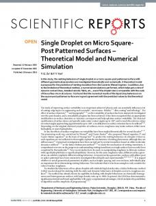
Fig. 1.

x

Kirchho vortex.

D U0 represents the fourth-order numerical dissipation in the  -direction de ned by D U0 j;k =   R j j2 R; 1  U0j;k with the dierence operator  U0j;k = U0j+1=2;k ;U0j;1=2;k . The Jacobian matrix of the  -direction ux can be di-

agonalized as @@F^U1 = R  R; 1 . The columns of R are the right eigenvectors of @@F^U1 and may be found in [29]. The eigenvalues of @@F^U1 de ne the diagonal matrix  = diag(u ; c ; u ; u ;p u + c ) , where u = uJ ;1 x + vJ ;1 y , and c = c (J ;1 x )2 + (J ;1 y )2 . The R is evaluated at the arithmetic average. D U0 j;k is de ned analogously. For our numerical experiments, the lter coecient  in the range of 0 <   0:05 exhibits the desired property. Whether a characteristic lter instead of a scalar lter is absolutely necessary, and the advantage of using the exact form of the Yee et al. ACM sensor or the wavelet sensor [26] will be addressed in a future paper.

4 Analytical Solution for Kirchho Vortex Sound The Kirchho vortex is an elliptical patch (Fig. 1) with semi-major axis a and semi-minor axis b of constant vorticity r  u = (0; 0; !)T rotating with constant angular frequency = (a+abb)2 ! in irrotational ow [11]. The 2D ow eld constitutes an exact solution of the 2D incompressible Euler equations [14]. The acoustic pressure generated by the Kirchho vortex is governed by the 2D Helmholtz equation, which can be solved analytically using separation of variables [16]. The normal velocity for an almost circular Kirchho vortex of radius R, i.e. a = R(1 + ), b = R(1 ; ), 0 <   1, can be approximated by [16] u
n  2R sin(2( ; t)): (16) Assuming a harmonic time dependence at the angular frequency 2 for the acoustic pressure p0 (r; ; t) = p^(r; )e;i2 t ; reduces the wave equation to the Helmholtz equation k2 p^ +
p^ = 0

5

with wave number k = 2 =c0. Separation of variables yields the solution for the Helmholtz equations p0 (r; ; t) =