High Order Window Functions and Fast Algorithms for Calculating Dyadic Electromagnetic Green’s Function in Multilayered Media. Tiejun Yu, Wei Cai+ Department of Electrical & Computer Engineering Duke University, Durham, NC 27708
[email protected] + Department of Mathematics University of North Carolina at Charlotte Charlotte, NC 28223
[email protected]
April 24, 2003 Abstract A type of bell-shaped compact high order window function ψ(x, y) is studied, and closed analytic and approximation formulas are derived for its Hankel transforms. Applications of these results are presented as fast algorithms for calculating dyadic Green’s functions for electromagnetic scattering in multilayered media. Numerical results in electromagnetics are provided to demonstrate the accuracy and efficiency of the algorithms. Keywords: Green’s function for multilayered media, Window function, Fourier transform, Hankel transform Fast algorithm.
Submitted to Radio Science, August 28, 2000
1
1
Introduction
The purpose of this paper is to derive closed-form formulas for the two dimensional Fourier transform of a bell-shaped radial symmetrical high order window function with compact support and show some of its novel applications in electromagnetic scattering. Such a window function was initially introduced in [18] and, in this paper, we will provide closed-form formulas for the Fourier transform of the window function itself and other two related functions used in the fast algorithms for calculating dyadic electromagnetic Green’s functions in multilayered media. More detailed numerical studies are presented in this paper to demonstrate the accuracy and efficiency of the proposed fast algorithms. We begin with a definition of the high order window functions. Referring to Fig.1, a compact radial symmetric bell-shaped function ψ a (x, y) with a support size a is defined as ½ (1 − ( aρ )2 )m , if ρ ≤ a ψ a (x, y) = ψ a (ρ) = (1.1) 0, otherwise. p where ρ = (x2 + y 2 ) and m > 0 is the order of the window function. In most cases, we will ignore the subscript a in ψ a (x, y), simply identify it as ψ(x, y) or ψ(ρ) with the understanding that the window function has a support size a. The two-dimensional Fourier transform of the above window function ψ(x, y) is e (kx , ky ) F {ψ (x, y)} = ψ Z ∞Z ∞ 1 ψ (x, y) ej[kx x+ky y] dxdy = 2π −∞ −∞
(1.2)
Changing x, y coordinates into polar coordinates in both the p spectral and spatial domain by: xq= ρ cos θ, y = ρ sin θ , kx = kρ cos α, ky = kρ sin α, ρ = x2 + y 2 , θ = arctan (y/x), kρ = kx2 + ky2 , α = arctan (ky /kx ), and also using the nth order of Bessel function Jn (z) 1 Jn (z) = 2π
Z
2π
cos (nθ − jz sin θ) dθ
(1.3)
0
the 2-D Fourier integral of (1.2) can be conveniently expressed in terms of a Hankel transform: Z ∞ e ψ (kρ ) = S0 [ψ (ρ)] = ψ (ρ) J0 (kρ ρ) ρdρ 0 Z a = ψ (ρ) J0 (kρ ρ) ρdρ.
(1.4)
0
e (kρ ) , and other two related The goal of this paper is first to derive closed form formulas for ψ e (kρ ), ψ e (kρ ) , which are to be used in the calculation of dyadic Green’s functions. functions ψ 1 2 e e ψ 1 (kρ ), ψ 2 (kρ ) are defined as Z a ˜ ψ (ρ) J1 (kρ ρ) ρ2 dρ (1.5) ψ 1 (kρ ) = S1 [ψ (ρ)] = 0
£ ¤ ˜ (kρ ) = S0 ψ (ρ) ρ2 = ψ 2 2
Z 0
a
ψ (ρ) J0 (kρ ρ) ρ3 dρ.
(1.6)
It should be noted that the window function ψ(x, y) defined above has very good properties in both the spatial and spectral domains. The window function ψ(x, y) of order m has a compact support and is smooth, especially when the order m is increased. In spectral domain, it has fast decay at high frequency and forms a low pass filter (LPF). Ideas of window functions are widely used in the area of signal processing. In this paper, we will derive the spectral formulas e (kρ ) , ψ e (kρ ) and ψ e (kρ ) in closed-form and, then use them to construct fast algorithms for for ψ 1 2 calculating Green’s function for multilayer structures, which has been long-term interest in the electromagnetic community [9] [8]. e (kρ ) , ψ e (kρ ) and ψ e (kρ ) The organization of the paper is as follows. Closed-form formula of ψ 1 2 in spectral domain are derived in the Section 2. Their applications in fast Green’s function computations are given in the Section 3. Section 4 presents detailed numerical experiments, and Section 5 draws the conclusion.
2
Theory
2.1
Analytical Formulas
e (kρ ) , ψ e (kρ ) and ψ e (kρ ) , we consider two cases: To derive the formula of ψ 1 2 Case One: kρ a < 1 : In this case, we use the Taylor expansion of the Bessel function Jn (z) , Jn (z) =
∞ X (−1)k k=0
k!
³ z ´2k+n 1 . (n + k)! 2
(2.1)
e ψ e and ψ e , by setting z = ρ/a, y = kρ a, we have According to the definitions of ψ, 1 2 ¶ Z aµ ³ ρ ´2 m e (kρ ) = ψ 1− ρJ0 (kρ ρ) dρ a 0 Z 1X m ∞ X 1 ³ yz ´2j i 2i+1 i 2 = a (−1) z Cm (−1)j dz j!j! 2 0 = a2
i=0 m ∞ XX
(2.2)
j=0
hi,j y 2j
i=0 j=0 aµ
Z e (kρ ) = ψ 1
1−
³ ρ ´ 2 ¶m
a 0 Z m ∞ XX 1
= a3 = a3
i=0 j=0 0 m X ∞ X
ρ2 J1 (kρ ρ) dρ
i (−1)i z 2i+2 Cm (−1)j
(2.3) ³ yz ´2j+1 1 dz j!(j + 1)! 2
ei,j y 2j+1
i=0 j=0
Z e (kρ ) = ψ 2
aµ
1− 0
³ ρ ´2 ¶m a
3
4
ρ J0 (kρ ρ) dρ = a
m X ∞ X i=0 j=0
3
fi,j y 2j
(2.4)
Where 1 m! 1 · 2j+1 · (m − i)!i!j!j! 2 i+j+1
hi,j = (−1)i+j ei,j = (−1)i+j
1 m! 1 2(j+1) i! (m − i)!j! (j + 1)! 2 i+j+2
fi,j = (−1)i+j
m! 1 1 · 2j+1 (m − i)!i!j!j! 2 i+j+2
Case Two: kρ a ≥ 1 : Here we use the fact that m 1 X 1 i e ψ (kρ ) = 2 (−1)i Cm Ii kρ (kρ a)2i
(2.5)
i=0
i = where Cm
Z 0
1
m! i!(m−i)! ,
Ii =
R akρ
xµ Jν (ax) dx =
0
J0 (u) u2i+1 du. Ii can be obtained by the identity
2µ Γ
³
aµ+1 Γ
ν+µ+1 2
³
´
ν−µ+1 2
´
(2.6)
+a−µ [(µ + ν − 1) Jν (a) Sµ−1,ν−1 (a) − Jν−1 (a)Sµ,ν (a)] . where a > 0, Re (µ + ν) > −1. If µ + ν or µ − ν is positive integer, the Lommel functions Sµ,ν (z) are Sµ,ν (z) = z µ−1
n X k=0
2 Γ (−ia + 1) Γ (−ib + 1) (−1)k ( )2k . Γ (−ia − k + 1) Γ (−ib − k + 1) z
(2.7)
where n = min(−ia, −ib), ia = (1 − µ + ν)/2, and ib = (1 − µ − ν)/2. For other values of µ, ν, we have the following asymptotic approximations [20] 4 Sµ,ν (z) ≈ z µ−1 3 F0 (1, ia, ib, − 2 ) z ½ 2 − ν2 (µ − 1) [(µ − 1)2 − ν 2 ][(µ − 3)2 − ν 2 ] = z µ−1 1 − + z2 z4 ¾ [(µ − 1)2 − ν 2 ][(µ − 3)2 − ν 2 ][(µ − 5)2 − ν 2 ] − + ··· . z6 where 3 F0 (1, ia, ib, − z42 ) is the hypergeometric function [20]. e (kρ ) , ψ e (kρ ). Similarly, we can derive formulas for ψ 1 2
4
(2.8)
2.2
Approximation Formulas
Based on the analytic formulas given above, we can obtain the following approximation formulas e (kρ ) , ψ e (kρ ) and ψ e (kρ ) . for ψ 1 2 Case One: kρ a < 1 : By truncating the series expansions in (2.2)-(2.4) , we get the following approximations in a nest format ¡ ¡ ¡ ¢¢¢ e (kρ ) = a2 Hm0 − y 2 Hm1 − y 2 Hm2 − y 2 (Hm3 − y 2 (Hm4 − y 2 (Hm5 − y 2 Hm6 ))) ψ
(2.9)
¡ ¡ ¡ ¢¢¢ e (kρ ) = a3 y Em0 − y 2 (Em1 − y 2 (Em2 − y 2 (Em3 − y 2 Em4 − y 2 Em5 − y 2 Em6 ))) ψ 1
(2.10)
¡ ¡ ¡ ¢¢¢ e (kρ ) = a4 Fm0 − y 2 Fm1 − y 2 (Fm2 − y 2 (Fm3 − y 2 (Fm4 − y 2 Fm5 − y 2 Fm6 ))) ψ 2
(2.11)
where m indicates the order of the window and y = kρ a . The 1st to 7th order window coefficients in (2.9-2.11) are calculated and summarized in the following tables. m Hm0 × 102 Hm1 × 103 Hm2 × 105 Hm3 × 107 Hm4 × 1010 Hm5 × 1012 1 25.00 20.83333 65.1041666 108.5069444 1130.28067 807.343336 2 16.6667 10.41667 26.04166 36.16898 322.9373 201.8358 3 12.50 6.25 11.574074 15.50099 121.1015 67.27861 4 10.00 4.166666 7.440476 7.750496 53.82288 26.91144 5 8.33333 2.9761905 4.650297 4.305831 26.91144 12.23247 6 7.1428571 2.2321429 3.100198 2.583498 14.67897 6.116237 7 6.250 1.7361111 2.170138 1.644044 8.562732 3.293358 m 1 2 3 4 5 6 7
Em0 × 103 416.66667 20.83333 12.5000 8.333333 5.9523809 4.4642857 3.4722222
Em1 × 105 260.41666 104.16666 52.083333 29.7619047 18.60119904 12.4007936 8.68055555
Em2 × 107 651.0416666 217.013888 93.0059523 46.5029761 25.8349867 15.500992 9.8642677
m 1 2 3 4 5 6 7
Fm0 × 103 83.33333 41.66666 25.00 16.6666 11.9047619 8.92857142 6.94444444
Fm1 × 104 104.16666 41.66666 20.833333 11.9047619 7.44047619 4.96031746 3.47222222
Fm2 × 106 390.625 130.20833 55.8035714 27.9017857 15.500992 9.3005952 5.9185606
Em3 × 109 904.224537 258.349867 96.8812004 43.0583112 21.5291556 11.7431758 6.85018588 Fm3 × 108 723.379629 206.679894 77.5049603 34.446649 17.2233245 9.39454064 5.4801487
5
Em4 × 1011 807.343336 201.835834 67.2786113 26.9114445 12.2324748 6.11623739 3.2933586 Fm4 × 1010 807.343336 201.835834 67.2786113 26.9114445 12.2324748 6.11623739 3.2933586
Em5 × 1013 504.589585 112.131019 33.6393056 12.2324748 5.09686449 2.35239899 1.1761995 Fm5 × 1012 605.507502 134.55722 40.3671668 14.678969 6.11623739 2.82287879 1.41144394
function Hm6 × 1015 4204.9132 934.4251 280.3275 101.9372 42.47387 19.60332 9.801662 Em6 × 1016 2336.06289 467.212579 127.421612 42.4738709 16.3361041 7.00118749 3.26722083 Fm6 × 1015 3270.48805 654.09761 178.390257 59.4634191 22.8705458 9.80166249 4.57410916
Case Two: kρ a ≥ 1. In this case by using Lommel function and Bessel functions,we have the following approximations, e (kρ ) = gm ψ where m is the order of the window, y = kρ a, gm are defined as follows: · ¸ a2 J1 (y) g1 = 2 −2J0 (y) + 4 y y · µ ¶ ¸ a2 8 −4 8 g2 = 2 J0 (y) + − 1 J1 (y) y y y y2 ·µ ¶ µ ¶ ¸ a2 48 24 6 g3 = 2 2 1 − 2 J0 (y) − 8 1 − 2 J1 (y) y y y y · µ ¶ µ µ ¶¶ ¸ 16 24 16 a2 182 J1 (y) g4 = 2 3 24y 1 − 2 J0 (y) + 2 1 − 2 3 − 2 y y y y y ¸ ·µ µ ¶¶ µ µ ¶¶ 96 40 1536 5 J1 (y) a2 1920 −2 + 2 3 − 2 J0 (y) + 36 − 2 1− 2 g5 = 2 4 y y y y y y y · µ µ ¶¶ µ µ µ ¶¶¶ ¸ a2 46080 24 80 12 96 20 24 g6 = 2 −1 + 2 1 − 2 J0 (y) + −1 + 2 3 − 2 5 − 2 J1 (y) y y5 y y y y y y a2 645120 g7 = 2 y y6 .
3
·µ µ µ ¶¶¶ µ µ µ ¶¶¶ ¸ 480 4 168 32 5 144 28 1 − 2 1 − 2 15 − 2 J0 (y) + −1 + 2 30 − 2 6 − 2 J1 (y) . y y y y y y y
e (kρ ) , similar closed forms can be obtained. e (kρ ), ψ For ψ 1 2
Application
In this section, we will apply the results from the previous section to improve the speed of fast algorithms, originally proposed in [18], for calculating dyadic Green’s functions for electromagnetic scattering in multilayered media. Integral equation(IE) based method of moments (MoM) is a popular technique for EM scattering [16], [3], [13], and parameter extraction of VLSI ,IC and their packages [6], [2], [14], [17]. One of the principal challenges in IE based MoM is the dyadic Green’s function calculation, which is usually very time- consuming for multilayer structures shown in Figure 2. The main reason is that the Green’s function G(ρ, z; z 0 ) for a multi-layered medium can be only obtained by a Hankel transform of the spectral Green’s function[10], [7],[11] as follows Z ∞ h ¡ ¢i ¡ ¢ 0 0 e e kρ , z; z 0 Jn (kρ ρ) kρn+1 dkρ . = G (3.1) G(ρ, z; z ) = Sn G kρ , z; z 0
The kernel of the Hankel transform contains a Bessel function which oscillates very fast (especially when the radial distance ρ between the source and observe points is larger) and decays 6
e is not well behaved when large number of layers slowly. Moreover, the spectral Green’s function G are involved and for high frequency scatterings. Much research has been done in the area of fast calculation of Green’s function for multilayered structures [9] [8]. Most of them uses the complex image method (CIM) based on a Prony method and the well-known Sommerfeld identity [15]. CIM works well for the Green’s function calculation when the source and field points are in the same layer and the frequency is limited to some appropriate range. However, in many cases, CIM does not work well due to the difficulty of pole extraction and especially in the case when source and field points are in different layers [21]. In [4] [5], an efficient evaluation of Green’s function was proposed based on the integration along the steepest-descent paths (SDP) for a half space problem. However, if more layers are involved, generally SDP will not be possible to find. We introduced a window function based acceleration algorithm in [18] [21]. But in [18], no e ψ e ,and ψ e were available, therefore the efficiency of the algoclosed-forms of window functions ψ, 1 2 rithm is affected by the expensive calculation of those functions. Here we will apply the formulas obtained above to improve the algorithms for Green’s function calculations. Algorithm 1 Fast Algorithm for G(ρ, z; z 0 ) : If ρ > 0, 1 [r2 W0 (ρ) − 2ρW1 (ρ) + W2 (ρ)] + O(a2 ) G(ρ, z; z 0 ) = M0 r 2
(3.2)
where h W0 (ρ) = S0
i ¡ ¢ e (kρ ) (ρ). e kρ , z; z 0 ψ G
(3.3)
e (kρ )](ρ) e ρ , z; z 0 )ψ W1 (ρ) = S0 [G(k 1
(3.4)
e (kρ )](ρ) e ρ , z; z 0 )ψ W2 (ρ) = S0 [G(k 2 Z πa2 M0 = M0 (a) = √ ψ(x, y)dxdy = m+1 x2 +y 2 ≤a
(3.5) (3.6)
A simpler algorithm is available if ρ ≥ a. Algorithm 2 Fast Algorithm for G(ρ, z; z 0 ) : For ρ > a, 1 G(ρ, z; z 0 ) = W0 (ρ) + O(a2 ) M0
as a → 0
(3.7)
e (kρ ) , ψ e (kρ ) and ψ e (kρ ), the contour integration As a result of the fast decay of the functions ψ 1 2 in the definition of W0 (ρ), W1 (ρ), and W2 (ρ) can be done efficiently with a much shorter contour in kρ space as depicted in Figure 3. In [18], an explicit estimate for the length of L4 of the contour e ψ e ,and ψ e will be used here. is given. The formulas developed in previous section for ψ, 1 2 4 To achieve O(a ) accuracy, using the idea of extrapolation with two different window sizes for Algorithm 2, we have the following algorithm.
7
Algorithm 3 Fast Algorithm for G(ρ, z; z 0 ) : For ρ > γa, 1 < γ < 2 G(ρ, z; z 0 ) =
1 γ2 1 [ W0 (ρ, a) − W0 (ρ, γa)] + O(a4 ) γ 2 − 1 M0 (a) M0 (γa)
(3.8)
For ρ ≤ γa, a similar O(a4 ) version of Algorithm 1 can be obtained.
4 4.1
Numerical Experiments Preliminaries
Before proceeding to the applications of the algorithms, we first check the accuracy of the closede ψ e and ψ e in Section 2.2. Computing ψ, e ψ e and ψ e by both the closed form expressions of ψ, 1 2 1 2 e e e form formulations derived in Section 2 and the definition of ψ, ψ 1 and ψ 2 given in Section 1, we obtain the relative error for all the closed forms given in Section 2.2 less than 10−9 . Figure 4 - 6 e (kρ ), ψ e (kρ ) and ψ e (kρ ) with different order m (window size a = 1), show the window functions ψ 1 2 respectively. Form the figures we can see that the windows in spectral domain form low pass filters (LPF). As the order m of the window functions is increased, the windows in spectral domain decay 1 e (kρ ), ψ e (kρ ) and ψ e (kρ ) is in an algebraic order of m+2 faster. In fact, the decaying order of ψ [18]. 1 2 k ρ
e ψ e and ψ e insures that a short integration contour L4 shown in Figure 3 can The fast decay of ψ, 1 2 be selected without sacrificing the accuracy of approximation Algorithm 1,2, and 3. To validate the accuracy and efficiency of the window acceleration algorithms, we first compare the Green’s functions by the fast algorithms and by direct Sommerfeld integration (DSI). Then, S-parameters extraction of microstrip circuits and VLSI is conducted with our codes [17] [18] (denoted as “Duke”) with the above fast Green’s function algorithms, and the Ansoft commercial software, “Strata” (denoted as “Ansoft”) with CIM techniques for Green’s function calculation. Also an application in subsurface near zone electromagnetic-induction (EMI) scattering is given, which involves a lot of Green’s function calculations. The size unit for all examples are meter (m). z = 0 is defined at the air-dielectric(earth) interface.
4.2
Comparison to DSI Green0 s Functions
In this test case, we will calculate the dyadic Green’s functions GA (ρ, z; z 0 ), GV (ρ, z; z 0 ) for a five layered medium. Four dielectric layers are used between the open air layer and a perfect electric conducting (PEC) ground plane. The relative dielectric constants for the four dielectric layers are, from top to bottom, ²1 = 9.6, ²2 = 12.5, ²3 = 2.4 and ²4 = 3.6 , respectively, and their corresponding thickness are h1 = 0.001, h2 = 0.003, h3 = 0.002 and h4 = 0.0015, respectively. Window ψ(ρ) of order m = 5 with support size a = 0.001 is used in Algorithm 1. Comparing with the contour used in the Green’s functions obtained with the DSI ( Gexac ), the L4 shown in Figure 3 is reduced more than 20 times for the fast algorithm (Gf ast ). Figure 7 contains the magnitude and imaginary and real parts of the scalar Green’s function GV (ρ, z; z 0 ) with z = −0.0035, z 0 = −0.0062. Figure 8 0 contains the component Gxx A (ρ, z; z ) for the vector potential A, again the magnitude and imaginary and real parts of this component are shown. The results from the fast algorithms demonstrate the high accuracy and efficiency of the algorithms for the Green’s functions.
8
4.3
Comparison to CIM Green0 s Functions
Figure 9 is an example for a microstrip band-pass filter. Mixed potential IE (MPIE) based MoM with RWG basis functions is used to obtain the S-parameters of the circuits. In this case, the 00 Green’s functions needed are two layer Green’s functions Gxx A (ρ, 0/0) and GV (ρ, 0/0). For Ansoft software, CIM is used to calculate Green’s function, while we use Algorithm 2 and Algorithm 3 with interpolation table techniques both in the spatial and spectral domain as suggested in [1]. For simple cases like this example, our code is as fast as Ansoft software, “Strata”. Figure 9 shows the computed S-parameters by both codes and the agreement is good. One of the most widely used elements in VLSI and its package is shown in the Figure 10. It is composed of two strip lines connected with a cylindrical via. Our MPIE MoM code and “Strata” are used to compute the S-parameters. The Green’s functions used in this example are more complicated than that in the above microstrip circuit. When MPIE based on MoM is applied, we need all the terms of dyadic Green’s functions GA (ρ, z/z 0 ) and Gv (ρ, z/z 0 ). Figure 10 is the computed results. Our code is about 10 times faster than “Strata” for this case due to the fast Green’s function calculation and mixed baiss functions [17] used in our MoM code.
4.4
Application in Subsurface Detection
Figure 11 shows a subsurface EMI scattering result with the fast Green’s function algorithm. The rigorous method of moments (MoM) and approximate extended-Born method (E-Born)[1][12] are used to model this three-dimensional (3D) problem. The models involve a lot of Green’s function computation[1]. Three methods are used to calculate the Green’s functions, they are CIM, DSI and window based acceleration algorithms (Window-G) proposed in this paper. An actual wideband EMI sensor, termed the GEM-3 [1], is used in the modeling. Three dielectric targets are buried underground. The dielectric constants of the three targets are εr = 3 while the earth is modeled as 5% water content Yuma soil with εr = 5 − j0.2, σ = 0.01s/m. Target one is a cube centered at (−0.5, 0, −0.14) with edge length = 0.12; target two is a cube centered at (−0.65, 0.6, −0.14) with the same edge length of target one; target three is a cylinder centered at (0.5, 0, −0.12) with a radius R = 0.16 and height h = 0.08. The EMI sensor moves above the earth surface at z = 0.02 in a monostatic detecting way and collects the induced voltage produced by the 3 dielectric targets. Figure 11 is the computed space-dependent induced voltages for the three targets. By examining the two “E-Born” results in Figure 11, the agreement indicates that the Green’s functions obtained by the CIM and the proposed fast algorithm ( Window-G) agree well. In fact, in the “CIM-G EBorn” result, there are two cases of Green’s functions, the first case of Green’s functions is used for the inside field and scattering out field. Thus, Green’s functions in this case have their source and field points in different layers, so they can not be calculated accurately by CIM, instead, DSI has to be used. The second case of Green’s functions is used in obtaining induced currents in the target by E-Born, Green’s functions thus have their source and field points in the same layers, they can be calculated by CIM. On the other hand, in the result of “Window-G E-Born”, all the Green’s functions are obtained by window based acceleration algorithms proposed in this paper. The good agreement is confirmed between the Window-G and DSI for calculating the Green’s functions, while DSI is much more time consuming. Comparing the two “E-Born” results and “MoM” result, and the real target distribution, we see that the highly efficient extended-Born method consistently yields space-dependent results that are in close agreement with the MoM reference solution. The EMI near zone signatures are not
9
only used to locate the buried targets, but also to provide information about the target’s identity which can be used for the inverse scattering.
5
Conclusion
e ψ e , and ψ e window functions are derived. Based on these formulas, The closed-forms formulas of ψ, 1 2 improved fast algorithms for Green’s function calculations in multilayered structures are proposed. The speed of the algorithms comes from two factors: the shorter integration interval and the e ψ e and ψ e . Compared with Prony based CIM, these algorithms have simple closed forms for ψ, 1 2 the advantages of no need for poles extraction, easy error control, robustness and applicability for arbitrary source and field layers. Numerical experiments have demonstrated the efficiency and accuracy of the algorithms.
Acknowledgment The authors would like to thank the support of a NSF grant CCR-9972251 for the work reported in this paper, thanks also are extended to Prof. Jiayuan Fang(UCSC), Prof.Lawrence Carin (Duke Univ.) and Dr. Xingchao Yuan (Rambus Inc.) for many interesting discussions.
10
References [1] Tiejun Yu,and L. Carin “Electromagnetic-Inductive Response of a Dielectric Void in a Soil Background”, IEEE Trans. Geoscience and Remote Sensing, vol. 38, no.3, pp. May, 2000. [2] W.Shi, J. Liu, N. Kakani and Tiejun Yu,. “A Fast Hierarchical Algorithm for 3-D Capacitance Extraction,” Proc., 35th DAC, San Francisco , pp. 212-217, June.1998, best paper award. [3] S.M.Rao, D.R.Wilton and A.W. Glisson, “Electromagnetic scattering by surfaces of arbitrary shape,” IEEE Trans. Antennas Propagat.,vol.AP-30, pp. 409-418, 1982. [4] T. J. Cui and W. C. Chew, “Fast evaluation of Sommerfeld integrals for EM wave scattering and radiation by three-dimensional buried objects,” Technical Report, Electromagnetic Laboratory, University of Illinois at Urbana -Champaign, Dec.1997. [5] T. J. Cui and W. C. Chew, “Efficient evaluation of Sommerfeld integrals for TM wave scattering by buried objects,” J. Electromagnetic Wave Appl., vol.12 pp.607-657, 1998. [6] K. Nabors and J. White, “Fastcap: A multipole accelerated 3-D capacitance extraction program,” IEEE Trans. Computer-Aided Design of Integrated Circuits Syst., vol.10, pp. 1447-1459, Nov.1991. [7] Tatsuo Itoh, Numerical techniques for microwave and millimeter-wave passive structures. John Wiley & Sons, Inc., 1989. [8] M.I.Aksun, “A Robust Approach for the Derivation of Closed-Form Green’s Functions” IEEE Trans. Microwave Theory Tech., vol.44, pp.651-658, May 1996. [9] Y.L.Chow , J.J.Yang, D.G. Fang and G.E.Howard, “A Closed-Form Spatial Green’s Function for the Thick Microstrip Substrate”, IEEE Trans. Microwave Theory Tech., vol.39, pp.588-592, Mar. 1991. [10] K. Michalski and D. Zheng, “Electromagnetic Scattering and Radiation by Surfaces of Arbitrary Shape in Layered Media, Part I: Theory” IEEE Antennas Propagat. , vol. AP-38, pp. 335-344, Mar.1990. [11] K. Michalski, J.R. Mosig “Multilayered Media Green’s Functions in the Integral Equation Formulations” IEEE Antennas Propagat. , vol. AP-45, pp.508-519, Mar.1997. [12] T.M.Habashy, R.W.Groom, and B.Spies, “Beyond the Born and Rytov approximations: A nonlinear approach to electromagnetic scattering,” J.Geophys. Res., vol.98,no. B2, pp.17591775,1993. [13] J. He, T.J. Yu, L.Carin , “Method of moments analysis of electromagnetic scattering from a general three-dimensional dielectric target embedded in a multilayered medium”, Radio Science, vol.35, No.2, pp.305-313, March, 2000. [14] C. H. Chan, R. A. Kipp,“Application of the complex image method to multilevel , multiconductor microstrip lines,” Int. J Microwave Millimeter-Wave CAE 7 , pp.359-367, 1997 John Wiley & Sons, Inc. [15] Sommerfeld A, Partial Differential Equations in Physics. New York: Academic Press., p.242, 1949. 11
[16] R. F. Harrington, Field Computation by Moment Methods. New York: Macmillian, 1968. [17] W. Cai, T.J. Yu, ”High Order Mixed RWG Basis Functions for Electromagnetic Scattering and Applications”, submitted and revised for IEEE Trans. Microwave Theory Tech., 1999. [18] W. Cai, T.J. Yu, ”Fast Calculation of Dyadic Green’s Function for Electromagnetic Scattering in the Multilayered Medium”, to appear in J.Comput. Phys., 2000. [19] J. Van Bladel, Singular Electromagnetic Fields and Sources, IEEE Press, New York, 1991. [20] H. Batman, Higher Transcendental Functions, Vol. I, II, McGraw-Hill, New York, 1953. [21] T.J. Yu, W. Cai, B. Zhu, “Fast Evaluation of the Sommerfeld Integrals for the Stratified Media Green’s Function with Field and Source Points in Different Layers”, IEEE Proceeding of Antenna and Propagation, APs, pp.472-475, 2000 .
12
Figure 1: High order window function ψ(ρ) with order m=1,3,5,7,9.
Figure 2: Multilayer structure with 3-D PEC objects buried in it.
Figure 3: Sommerfeld integral path (SIP). 13
e ρ )|). Here a = 1, the order m = 1, 3, 5, 7. Figure 4: Window functions log(|ψ(k
e (kρ )|), here a = 1, the order m = 1, 3, 5, 7. Figure 5: Window functions log(|ψ 1 14
e (kρ )|). Here a = 1, the order m = 1, 3, 5, 7. Figure 6: Window functions log(|ψ 2
15
Figure 7: Scalar potential Green’s functions GV (ρ, z; z 0 ).of a five layered medium. Gf ast is obtained by our window accelerating algorithm, Gexac is obtained by direct Sommerfeld integration. L4 used in Gexac is 20 times longer than that used in Gf ast . f = 1GHz.Window function ψ(ρ) with order m = 5.
16
0 Figure 8: Vector potential Green’s functions Gxx A (ρ, z; z ) obtained by window based accelerating algorithm, noted by Gf ast , and by direct Sommerfeld integration , noted by Gexac .
17
Figure 9: Compared S-parameters of a microstrip band-pass filter. The dielectric thickness h = 0.1mm, and εr = 12.9. The geometry and its discretization is also provided here.
18
Figure 10: Compared S-parameters of the structure composed by two striplines connected with a via. Via diameter d = 0.08485mm, both of the strip lines with width b = 2.4mm, length a = 4.8mm. Port 1 defined by two points (unit mm): (−3.6, −1.2, −0.795), (−3.6, 1.2, −0.795);Port 2 defined by two points : (3.6, −1.2, 0), (3.6, 1.2, 0). The mesh used is also inserted in the figure.
19
Figure 11: The contour line of the space-dependent induced voltages of EMI sensor moving around the earth surface. MoM and extended-Born method (E-Born) are used to model the half space EM scattering. Three methods are used to caculate the Green’s functions, they are CIM, DSI and window based acceleration aglorithms(Window-G) proposed in the paper. Three dielectric targets are buried in the earth with 5% water content. f=100KHz
20