The effect of turbulent mixing at the water-bed interface will be included. The 2D model is then combined with the 3D model to reduce the computational cost.
Department of Civil, Geo and Environmental Engineering
High Performance Computing of Coupling 2D and 3D Numerical Modeling of Flood Propagation and its High Performance Interface and Visualization Ginting, Bobby Minola – Chair for Computation in Engineering
Finite Volume Method • Two Dimensional: 2D Shallow Water Equations (with the modules of non-Riemann solvers (artificial viscosity technique and central upwind), Riemann solver (HLLC method), evaluation of viscous fluxes and turbulent terms. • Three Dimensional: 3D Navier Stokes Equations with Boussinesq approximation and incompressible flow. 𝑪𝒐𝒏𝒕𝒊𝒏𝒖𝒊𝒕𝒚 𝒆𝒒𝒖𝒂𝒕𝒊𝒐𝒏
Progress: Test Cases (2D)
m/s
1. The jet forced viscous flow in a circular reservoir Velocity Vector
Velocity Contour
The program can simulate the jet viscous flow very accurately. As well as shown in the laboratory results, along the center of the channel the numerical model yields the velocities which are higher than the velocities at the wall. The recirculation flow zones occur at both parts of the wall, where the velocities in these areas are very small.
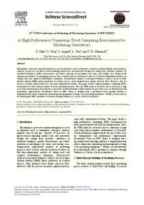
2. The 90 degrees dam-break case Unstructured Triangular Mesh Point G1 Point G4 Point G3
3.415 m
This work aims at providing the accurate numerical model in predicting the flow characteristics including depth and velocity in all directions such as flood wave propagation and spreading and velocity distribution profile. Expected Research Output: • Combination of two and three dimensional numerical modeling with wet and dry treatment in simulating the inundation process. Since most of numerical models fail when flow discontinuity occurs, then the efficient and simple treatments have to be developed. • The turbulent mixing at interface between water and bed or structure interaction is expected to be calculated. • The proper user interface tool for giving the very detail input of the numerical modeling. These are unstructured mesh models with strong ability in resolving domain with complex geometry and the high performance visualizations of the numerical modeling results. State of the Art In reality the true dynamics of vertical convection are based on non-hydrostatic process. Most of the developed codes are hydrostatic which could not describe the true characteristics of fluid motion, for example the vertical velocity distribution along the depth. In this research, the non-hydrostatic approximation will be developed and included in the flood propagation modeling. The effect of turbulent mixing at the water-bed interface will be included. The 2D model is then combined with the 3D model to reduce the computational cost. Research Questions and Hypotheses • How significant do the turbulent mixing at water and bed or structure interface affect the evolution of flood waves? Hypothetically, these stresses will be significant to the accuracy of the evolution of surface water waves. • How is the shape of the vertical velocity distribution profile due to bed stresses? Hypothetically, these bed stresses effects will be significant to the shape of the vertical velocity distribution profile. • Is the interchanging process from dispersion to nonlinearity simulated well and stably in a straightforward fashion?
2.44 m
Overview
4.415 m 2.39 m
meter
Depth Propagation T=1 s
meter Depth Propagation T=3 s
In dealing with the high discontinuity problem, the artificial viscosity is used. This case deals with the high discontinuity problem. At T=0s, the water is only located at the rectangular reservoir and then the gate is suddenly opened. The numerical model is in very good agreement with the laboratory results.
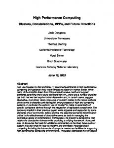
3. The hydraulic jump over a spillway
The numerical model deals with the hydraulic jump (high discontinuity problem). The numerical model is in very good agreement with the analytical results.
The Future Works This research has been being started since October 2015 and the 2D model was successfully developed. In the next step, the 3D model will be developed and then combined with 2D.
div U dV = 0 CV
𝑴𝒐𝒎𝒆𝒏𝒕𝒖𝒎 𝒆𝒒𝒖𝒂𝒕𝒊𝒐𝒏
CV
∂ui dV + ∂t
div ui U dV = − CV
i = 1, 2, 3 or x, y, z
CV
∂h g dV + ∂xi
div µ grad ui dV + CV
SMi dV CV
References 1. Ginting, B.M., (2011), “Two Dimensional Flood Propagation Modeling Generated by Dam Break Using Finite Volume Method”, Master Thesis, Bandung Institute of Technology, Indonesia. 2. Jameson, A., Schmidt, W., and Turkel, E. (1981). “Numerical Solution of the Euler Equations by Finite Volume Methods Using Runge-Kutta Time-Stepping Schemes.” AIAA 14th Fluid and Plasma Dynamic Conference.