Abstract-We discuss an extension of the pencil-of-functions method, namely, the use of band-pass processing filters, and show that this leads to considerably ...
IEEE TRANSACTIONS ON ACOUSTICS, SPEECH, AND
SIGNAL PROCESSING, VOL. ASSP-34, NO. 4, AUGUST 1986
997
Numertransforms exist if and only if (5) is held and there is a solution of [6] J. Hekrdla,“Indextransforms of N-dimensionalDFT,”in Berlin,Germany:Springer-Verlag,submitted for ischeMathematik. (7). Equations (8) and (9) describe their general form. publication. One of the promising applications of such transforms follows from the fact that fast compu.tationa1 algorithms of DFT and CC often map rn-dimensional DFT and CC operators on n-dimensional ones. The implementation of such index transforms can be made by subroutines in the case of general computer. If this method is used for microprocessors, it.is probably more convenient to store corresponding addresses of indexes in aROM memory. High-Performance Signal-Modeling by Pencil-ofThe general equations describing the index transforms make it Functions Method: Band-Pass Case possible to find some new results which do not follow from CRT. One of these are index transforms f r , A such that f l = A. This V. K.JAIN AND T. K.SARKAR solution can simplify the softwareof a computer or reduce memory requirements in a microprocessor implementation. For example, in the caseof transform of a one-dimensional DFT operator on a fourAbstract-We discuss an extension of the pencil-of-functions method, dimensional one, the conditionf, = can be achieved for lengths namely, the use of band-pass processing filters, and show that this leads M = 570,714, 858, 1170, * , pointDFT’s.Similarsolutions also exist in the case of multidimensional DFT operators. For ex- to considerably enhanced modelingof band-pass signals. The theory of . suchprocessingispresentedandanexampleisgivenwhichdemon2,u3 2u4)6, u2 = (324, 24 ample,relations u1 = (3u2 4 ~ describe ~ ) index ~ transforms fi = A of two-dimensional 6 X 6 strates the efficacy of the technique at moderate to high levelsof data noise. point DFT on four-dimensional 2 X 2 X 3 X 3 point DFT. Unfortunately, the general method solving (7) has not been found and it is very probable that such a method does not exist. MoreI. INTRODUCTION over, a rule testing the solvability of (7) is known only in some Methods for modeling a time domain signal by a rational transfer special cases. Nevertheless, in many practical applications, (5)-(7) function range from the early Prony method to gradient methods, make it possible to design index transforms relatively without difand from the maximum likelihood method, to the recent singularficulties. value decomposition (SVD) method [ 11. We have expiored the The first step of the design contains the choice of numbers M i , pencil-of-functions method [ 2 ] , [3], and have found it suitable for Nj which satisfy (5). From the elementary theory of congruencies, use at practical values of SNR’s [4]. It appears that when weighed it follows that some combinations of Mi’s, Nj’s result in the unin terms of performance and computational feasibility, the singusolvability of (7). For example, if there exists Nj such that lar-value decomposition method and the pencil-of-functions method are perhaps two of the more practical techniques for signal modeling,althoughwemustalsoacknowledgeothercontemporary modeling approaches notably Burg, Pisarenko, and the high-order Yule-Walker equations techniques. As stated above, a significant advantage of the pencil-of-functhen (7) is unsolvable. A similar rule results from the formal interchange of M * N , rn * n in (1 1). Unfortunately, the rule based tions method is its high performancein the presence of noise. This on (1 1) does not guarantee the solvability of (7), however, it re- advantage is realized by creating a set of basis functions that are A cascade of filtersisused duces the number of possible combinationsof Mi’s, Nj’s. Further, rich inthehigh-SNRfrequencies.’ in many cases, (6) reduces the number of combinations of vaji in which, when excitedby the given data signal, generhtes at its nodes such a way that (7) can be solved heuristically or allows us to use the basis functions. In [4] each of the processing filters was a firstorder filter Q(z) = 1/(1 - qz). Each filter in the cascade processes a computer. From the theoretical pointof view, it is interesting that the con- its input in backward time. Further, when q is positive, as was the ditions of the existence of index transforms in both cases (DFT andcase in the examples of [4], then Q(z) acts as a low-passfilter; the set high SNR provided the given CC) are identical and are equivalent to the solvability of ( 5 ) and cascade then produces a basis with data signal itself has a spectrum concentrated at the low end. In (7). Theorem 2 then describes the interrelationship between DFT and CC index transforms and states one-to-one correspondence be- this corfespondence, we extend the previous results to the case of a cascade of alternation of processing filters Q,(z) = (1 - rz)/(l tween them. Further, it was shown that the symmetries following from (10) have a general character. It means that if one has func- - q l z - q2z2)and Q2(z) = z . This extension makes it possible to achieve high-performance estimation for signals whose spectral entions satisfying (3), then these functions are bijective and satisfy ergy is concentrated in a band other than simple low or high bands. (10). These results can give insight into existing algorithms and extend new possibilities. 11. GENERATION OF BASIS SIGNALS It is convenient to present the results first for the case where the REFERENCES data are assumed noiseless and the extent of the signal is taken to R. C. Agarwal and J. W. Cooley, “New algorithms for digital conbe singly infinite, i.e., N = 00. The signal is then representable as volution,” IEEE Trans.Acoust.,Speech, Signal Processing, vol. ASSP-25, pp. 392-410, Oct. 1977. Manuscript received August 15, 1983; revised December 30, 1985. This J. H. McClellan and C. M. Rader, Number Theory in Digital Signal Processing. EnglewoodCliffs,NJ:Prentice-Hall,1979,pp.21-50. of NavalResearchunderContract workwassupportedbytheOffice D. P. Kolba and T. W. Parks, “A prime factor FFT algorithm using N00014-79-C-0598. high-speed convolution,” IEEE Trans. Acoust., Speech, Signal ProV. K. Jain is with the Departmentof Electrical Engineering, University cessing, vol. ASSP-25, pp. 281-294, Aug. 1977. of South Florida, Tampa, FL 33620. C. S. Bums, “Indexmappingsformultidimensionalformulationof T. K. Sarkar is with the Department of Electrical Engineering, Rochthe DFT and convolution,” IEEE Trans. Acoust., Speech, Signal Pro- ester Institute of Technology, Rochester, NY 14461. cessing, vol. ASSP-25, pp. 239-242, June 1977. IEEE Log Number 8608146. ‘That is, the basis functions are so chosen that they have large spectral D. F. Elliott and K. R. Rao, Fast Transforms, Algorithms, Analyses, Applications. Neb York:Academic,1982,pp.99-145. content at frequencies at which the original signal has high SNR.
-
+
+
+
+
0096-3518/86/0800-0997$01.OO 0 1986 IEEE
998
IEEE TRANSACTIONS ON ACOUSTICS, SPEECH, AND SIGNAL PROCESSING, VOL. ASSP-34,
NO. 4, AUGUST 1986
It is clear that yo and y 1 are linearly independent, whereas y o , y l , and y2 are linearly dependent. O,(d = I1 - rz)/(l
- 912 - q*22)
Fig. 1 . Filter cascade consisting of band-pass filters and unit delays.
Reason for the Particular Choice of Q l (z) and Qz(z) Lemma 1 also sheds light on the reason for the particular choice of the filters Q , and Q2. To state it more explicitly, we have used the filter combination Q l and Q2 as a second-order filter with a twostate output. A theoretically more general, but effectively equivalent, strategy would be to use Q 1 ( z )= (a bz)/(l - q l z - q2z2), and Q2(z) = ( c dz)/(l - q , z - q 2 2 ' ) , ( c , d) not a scalar multiple of (a, b), with no apparent advantage or disadvantage.
+
+
111. DETERMINATION OF PARAMETERS VIA PENCIL-OF-FUNCTIONS THEOREM FOR RATIONALLY REPRESENTABLE SIGNALS We begin this section with the consideration of a pencil set. For where ai and bi are the numerator and denominator parameters, convenience of notation, we let R(z) = (1 - rz) and D(z) = (1 respectively; z, are the signal poles, and Km the corresponding resq l z - 4 9 ' ) so that the processing filterQl may be written as Q,(z) idues. The basis signals are generated by processing the data signal = R(z)/D(z).Also, we will denote by Z(z) the inverseof Q 1 ( z ) i.e., , through the filter cascade shown in Fig. 1. Thus, letting yo@) = Z(z) = D(z)/R(z). y ( n ) , we successively have Lemma 2: The set i = o , . . . E 1 I(Z) Yl(Z) - yo(-?),yz(Z) - Z y ~ ( z )I(Z) , y3(Z) - yz(Z), y4(Z) (2a) ~ 2 +iI (n) = QIt ~ 2(n)l? i '2 - Z Y d Z ) , * * * , KZ) Yp-I(Z) - Yp-2(2), Yp(z) - ZYp-l(Z) ~2i+z(n= ) Q 2 t ~ 2 i + I ( n ) l , i = 0, . * . - 1 (2b) (5) '2 is linearly dependent if and only if z equals z,, i.e., one of the where we have used the notation Q [ ] to denote the operation of the filter Q on theargument signal, starting at infinite time, and we poles zm of the signal. Dejnition: Define the p 1-dimensionalGram(correlation) have set yk(co) = 0 for all k . Note that matrix Q , ( d = (1 - rz)/(? - q l z - q2z2) (34 (Yo,Yo) * * * ( Y o , Yp) Q2(4 = z (3b) F= :. .: .: are both anticausal filters. The reason for the above choice will be discussed later. The family of signals generated abovewill be called information N- 1 signals. For the case of rational stable' signals [4], this family is also a basis set, i.e., y ( n ) lies in the subspace spanned by y l ( n ) , * ,y i ( n ) . We have assumedp tobe even for convenience. This or equivalently, observation follows immediately from the following lemma. N- 1 Lemma I : If y ( n ) is rational stableof orderp with poles z,, then the corresponding information signals are also stable rational of order p with poles zm: where
r
The proof of this lemma follows immediately from the fact that the response of an anticausal filter Q(z) to the input zl,is Q(z,) 2:.
From the lemmaitis easily observedthatthe y p- I is linearly independent, while the set yo, . dependent. For example, if p = 2
*
set yo, * * . , , yp is linearly
'The signal y ( n ) is said to be rational [4] if it is the impulse response of a rational transfer function such as (1); additionally, it is said to be stable if all of the poles lie within the unit circle.
+
;
Y(n) = tYo(n) Y i ( 4 * * * Y p ( 4 1 T . (9) We can now apply the pencil-of-functions theorem of [2] to obtain the central theoretical result of this section. Note that a statement of the pencil-of-functions theorem was also given in[ 4 ] . Theorem I: The poles of the impulse response y ( n ) must satisfy the equation P i=O
where Mi are signed square-roots of the diagonal cofactors of the Gram matrix F [2]. In (10) the notation [x] denotes the truncated integer value of x. The proof of the theorem follows immediately upon application of the pencil-of-functions theorem to the set (5). The signs of the square roots are taken to be the signs of the cofactors of the first row of F. Now the denominator of the model A(z) is obtained by normalizing the leading term of the polynomial in (10). To clarify the notation, we explicitly expand (10) for the case p = 2 :
The numerator parameters can now be found by the method of least squares, specifically by solving the linear equation Cb = c
(12)
999
IEEE TRANSACTIONS ON ACOUSTICS, SPEECH, AND SIGNAL PROCESSING, VOL. ASSP-34, NO. 4, AUGUST 1986
TABLE I EFFECT OF RECORD LENGTH: SECOND-ORDER SIGNAL
N
100
whereb = [bobl and
4
20
50
0.62619 Estimated0.63639 0.63639 Poles rtj0.63640
kj0.63638
. bP-,lT, c = [cocl
*
TABLE I1 BIASAND STANDARD DEVIATION OF ESTIMATED DENOMINATOR PARAMETERS, POLES, AND NORMALIZED MEAN-SQUARE(SNR ERROR = 15 dB)
*
~0.62723
BIIS. STANDARD DEV.
( 13a)
(Ui, y ) .
(13b)
Here uidenotes the impulse response of z-'/A(z). Note that ui(n) = u(n T i ) where u(n) is the impulse response of l/A(z). All innerproducts are summed from n = 0 to N - 1.
I
SVD Pencll-of-functions Method (0-12) Metnad ( p - 4 ) (only 4 pole3 shown)
Covariance
-0.0110. 0.0180, -0.0045, 33.0172.
1.3714, 0.0579 -2.4578. 0,0920 2.2339, 0.0941 -0.7843. 0,0642
Bandpass
cP-,IT, and C = [c~];
cij = (Ui, U j )
ci =
Parameter or Pale
0.0176 0.0341 0.0317 0.0156
-0.0612, 0.1396, -0.1344. 0.0608,
0.0254 0.0462
-0.0198, 0.0093, -0.0107. 0.0156,
0.0051 0.0072 0.0018 0.0074
0.0414
0.0186
I
I
0.0313. -0.0052. -0.0258, 0.0187,
0.0017 0.0068 0.0080 0.0075
0.0350,
0.0157
Method
(p-4)
I
I I
I
not computed
0.0701,
0.0347
inator parameters are given in Table 11. For the pencil-of-functions method and the SVD method, the biases and standard deviations of the poles are also given in Table 11; they are not computed for the covariance method because of the wild scatter. The model order was taken to bep = 4 and the number of the data points used were N = 100. Note that the model order for the SVD method is actually 12 although only four poles associated with the largest singular values (and the corresponding denominator parameters) are listed in Table 11. This overmodeling is essential for the SVD method to A Second-Order Example obtain satisfactory results. It is evident from TableI1 that the penConsider the signalx(n) = 0.9" sin (0.7854n). Note that the true cil-of-functions method exhibits high performance in pole estimapoles are 0.63639 f j0.63640. Results obtained from various rec- tion. ord lengths are given in Table I; Ql(z) was 1/(1 - 1.22 0 . 7 ~ ~ ) . Finally, we consider the modeling effectiveness of band-pass s pencil-of-functions method at SNR less than 10 dB; we choose V. SIMULATIONEXPERIMENT = 0.2 so that SNR = 9 dB. The bias and standard deviation in the A simulation example is presented in this section. It is shown estimation of the poles are given below: thatatmoderately high levelsofnoisethepencil-of-functions method yield quite accurate results. At high levels of noise, the 0.0131 0.0723, Re[z(l)] degradation is noticeable; however, acceptable values of meansquare errors are still achieved, and the estimated poles have reaIm[z(l)l -0.0265, 0.0106 sonable variances as demonstrated by scattergrams. Example I : Consider the signal
IV. EFFECTOF MISSINGTAIL As discussed in [4] it is very difficult to assess the effect of tail truncationanalytically.Wewillthereforepresenttheresultsof simulation on a simple example. It is safe saytothat the best results areobtainedwhenthesignalhasdampedouttozerobefore n reaches N - 1.
+
with n = 0,
*
, 99. The signal to be tested is formed as x(n) = y(n) + sw(n)
Re[z(3)]
-0.0629,
0.0138
where w(n) is a zero-mean, unit variance, uncorrelated noise se0.0180. Im[z(3)] -0.0656, quence. The positive scalars is chosen to be0.1 so that the signalAlthough the estimation accuracy has understandably degraded, the to-noise ratio is 15 dB.3 poleshaveshiftedsomewhatgracefully.Also, we observethat The signal was tested by the following methods. while the bias is large, the s.d. is still small. 1) Theband-passversion of pencil-of-functionmethod.The processing filter Q, was chosen to be Q , = (1 z-')/(l - 1.222-1 Before leaving~thissection, we must remark that in the above examples no noise correction was applied. Needless to say, the O.~Z-~). performance would improveif a noise correction procedure similar 2) The singular-value decomposition method as developed in to that in [4] were used. [I]. 3) The all-pole covariance method. We remark that the poles thus obtained would be identical to thoseby the Prony method. VI. SELECTIONOF PROCESSINGFILTERQ,(z) Forty simulation runs, each with a different sample of noise, were performed. The biases and standard deviations of the denom- We have remarked that the filter Q, should beso selected that it peaks in the frequency band where the signal itself has a high SNR. This is not a difficult requirment to satisfy if a general idea about the signal spectrum is available to the user. In this section we give 3The SNR is defined as the average power of the signal to the average some guidelines for a quick selection of this processing filter. Conpower of the noise over the time frame considered.
+
+
lo00
IEEE TRANSACTIONS ON ACOUSTICS, SPEECH, AND SIGNAL PROCESSING, VOL. ASSP-34, NO. 4, AUGUST 1986
sider first the filter function
-1- -
~ ( z ) 1 - qlz
-
1 q2z* = (I - y P z ) ( l - ye-j‘z)
Corrections to “Finding the Polesof the Lattice Filter” (14)
where =
-4,
COS
e
(15)
= q,/2?.
To a first appr~ximation,~ theresonantpeakfrequency,the bandwidth, and the lower and upper cutoff frequencies are given by fo = e12~
B = (1
-
fi
=f o -
fi
=f o
$/a
+ Bl2.
q2 = -(I -
- fiN cos
K(f2
G
2
AND
ALLAN 0. STEINHARDT
In the above paper’ there are the following corrections on 1330. The formula for the phaseof zk in column 1 should read arg (2,) = lim arccos
(-(G~T;)
p.
+G~))/~IZ~I)
m+m
(a minus sign was missing). The equation for No should be labeled equation( 3 ) . The exponent in the formula for Sj should be 2J-‘.
B/2, (16)
Working back, giventhe cutoff frequencies, the denominatorparameters of the filter can be found from the formulas 4’ = 2(1 -
WILLIAM B. JONES
(.(h + h)),
-A)).
Manuscript received February 17, 1986. W. B. Jones is with the University of Colorado, Boulder, CO 80302. A . 0. Steinhardt is with M.I.T. Lincoln Lab, Lexington, MA 021730073. IEEE Log Number 8608239. ‘W. B. Jones and A. 0. Steinhardt, IEEE Trans. Acoust., Speech, Signal Processing, vol. ASP-33, pp. 1328-1331, Oct. 1985.
( 17)
Now, a zero can be placed in the numerator to form Q , ( z ) .In fact, for most purposes the zero may be placed either at 1 or - 1. If the signal has low-frequency drift, a zero at 1 is recommended, otherwise a zero at -1 should be used. Thus, Q , ( z ) = (1 f z ) / D(z), thereby completing the processing filter design. Using the aboveguidelines,theprocessing filters forexample 1 were designed. It is useful to point out that the filter cascade of Fig. 1 is not used here as a prefilter to be followed by a modeling procedure. Indeed, it is well known that prefilters introduce distortion in the results of the algorithm. Recall from Section I11 that exact paramof Q, in the eter values are recovered regardless of the choices absence of noise (and with N sufficiently large). However, when noise is present, proper choice of Q results in a good basis set and correspondingly robust estimation of the parameters.
Structured Fast Hartley Transform Algorithms C.P.
KWONG
AND
K. P. SHIU
Abstract-The flowgraph originally proposed for the computation of the radix-2 fast Hartley transform (FHT) is restructured for clarity and ease of implementation with hardware and software.By applying the transposition theorem to the newly formed flowgraph (which correspondsto a decimation-in-timealgorithm),adecimation-in-frequency algorithm with a similar flowgraph is obtained. The number of operations for the two algorithms is the same because of an existing symmetry, which is also identical to that of another FHT algorithm recently proposed.
VII. CONCLUSIONS I. INTRODUCTION We have extended the pencil-of-functions technique to the case In 1942 Hartley proposed a Fourier-like integral transform that where the signal spectrum is concentrated ainband of frequencies. Bracewell [2] It was shown that second-order processingfilters together with unit possesses a real kernel [l]. After some 40 years, Hartley delays yield a satisfactory cascade forproducing-by processing in presented the discrete versionof the transform, the discrete transform (DHT), and later the fastHartley transform (FHT) [3]backward time-the basisfunctions. A simulationexamplewas given to demonstrate that high performancein pole estimation can an analogy of the well-known fast Fourier transform (FFT). The be achieved with this method. Furthermore, thisefficacy is achieved same transformation has also been studied by Wang [4], [5] and named the W transform without referring toHartley. Most rewithout resorting to overmodeling. cently, the fast computation of the Hartley transform has been extended to include the radix-4, split radix, prime factor, and WinoREFERENCES grad algorithms [6]. [l] R. Kumaresan and D. W. Tufts, “Estimating the parameters of expoIn [3], where the radix-2 FHT algorithm is developed, a flownentially damped sinusoids and pole-zero modeling in noise,” IEEE graph for computing an 8-point DHT and a table of equations for Trans.Acoust.,Speech, Signal Processing, vol. ASSP-30, pp. 833- computing a 16-point DHT are shown. However, since neither the 840, 1982. flowgraph nor the table is well structured, not only that implemen[2] V. K. Jain, “Filter analysis by use of pencil-of-functions: Part I,” tation with hardware or software is difficult for high-order FHT, IEEE Trans. Circuits Syst., vol. CAS-21, pp. 574-579, Sept. 1974. certain properties of the algorithm have been hidden. For instance, [3] -, “On system identificationandapproximation,”FloridaState it has been thought that theoriginal decimation-in-time (DIT) FHT Univ., Tallahassee, Eng. Res. Rep, SSI1, 1970. [4] V. K. Jain, T. K. Sarkar,and D. D. Weiner, “Rational modeling by algorithm would work more slowly than a recently proposed deci171. However, it will be pencil-of-functions method,” IEEETrans.Acoust.,Speech, Signal mation-in-frequency (DIF)algorithm Processing, vol. ASSP-31, pp. 564-573, June 1983.
4This approximation is good only when 1 - y is small. However, the objective here is not to achieve exact -3 dB cutoff at fi and f2; rather it is to create a filter which emphasizes the spectrum betweenf, andf,.
Manuscript received August 12, 1985; revised December 9, 1985. The authors are with the Department of Electronics, the Chinese University of Hong Kong, Shatin, N.T., Hong Kong. IEEE Log Number 8608136.
0096-3518/86/0800-1000$01.00 O 1986 IEEE