EUROGRAPHICS - IEEE VGTC Symposium on Visualization (2005), pp. 1–9 K. W. Brodlie, D. J. Duke, K. I. Joy (Editors)
High-Quality Volume Rendering with Resampling in the Frequency Domain Martin Artner† , Torsten Möller‡ , Ivan Viola† , and Meister E. Gröller† † Institute
of Computer Graphics and Algorithms, Vienna University of Technology, Austria of Computing Science, Simon Fraser University, Vancouver, Canada
‡ School
Figure 1: The Stanford Head, Tooth, and the Stanford Bunny rendered with our new frequency domain based method.
Abstract This work introduces a volume rendering technique that is conceptually based on the shear-warp factorization. We propose to perform the shear transformation entirely in the frequency domain. Unlike the standard shear-warp algorithm, we allow for arbitrary sampling distances along the viewing rays, independent of the view direction. The accurate scaling of the volume slices is achieved by using the zero padding interpolation property. Finally, a high quality gradient estimation scheme is presented which uses the derivative theorem of the Fourier transform. Experimental results have shown that the presented method outperforms established algorithms in the quality of the produced images. If the data is sampled above the Nyquist rate the presented method is capable of a perfect reconstruction of the original function. Categories and Subject Descriptors (according to ACM CCS): I.3.3 [Computer Graphics]: Picture/Image Generation
1. Introduction and Related Work The resampling of discrete signals is an important part of any volume rendering algorithm. The numerically best implementation of volume rendering is the ray casting approach introduced by Levoy [Lev88]. For every pixel in the final image a viewing ray is cast into the scene. Numeric integra-
† {artner | viola | meister}@cg.tuwien.ac.at ‡
[email protected] submitted to EUROGRAPHICS - IEEE VGTC Symposium on Visualization (2005)
tion of the volume along the viewing rays is performed. This requires the computation of equidistant sample points along each viewing ray. The quality of the resulting image depends directly on the resampling filter used in this stage of the rendering process. Research has been done to improve the design of these spatial domain filters [MMK∗ 98], and to evaluate and compare the quality of the reconstruction [ML94]. As a basic principle all of these filtering methods are approximations of the sinc filter, which provides the ideal signal reconstruction. Unfortunately the sinc filter has infinite
2
Artner et al. / High-Quality Volume Rendering with Resampling in the Frequency Domain
extend in the spatial domain, therefore it is usually dismissed as a theoretical solution. However, the frequency domain representation of the sinc filter is a simple box filter. This leads to the assumption that volume rendering with sinc filter quality is possible if the resampling is done in the frequency domain. The Fourier transform was introduced to volume rendering by Dunne et al. [DNR90]. The proposed algorithm, later referred to as frequency domain volume rendering (FDVR), or Fourier volume rendering (FVR), was further established by Malzbender [Mal93], Levoy [Lev92] and Totsuka and Levoy [TL93]. The FVR method is based on the projection slice theorem of the Fourier transform, which states that projection in the spatial domain is equivalent to slicing in the frequency domain. If the size of the volume is N 3 , the computational expense of FVR is O(N 2 logN) as compared to O(N 3 ) of other rendering methods. Therefore the computational complexity of frequency domain volume rendering is lower than that of other traditional volume rendering approaches. Unfortunately even with the most recent improvements by Lee et al. [LDB96], Westenberger and Roederik [WR00] and Entezari et al. [ESMM02] which have added lighting effects, this method generates only “x-ray” like images. The lack of occlusion and support of transfer functions are the major drawbacks of this method. In this paper we utilize the shifting theorem, the packing theorem (also known as zero-padding), and the derivative theorem [OS89]. With these theorems we are able to perform volume rendering using the ideal sinc filter. Our method is conceptually based on the shear-warp factorization introduced by Lacroute and Levoy [LL94]. The essence of shearwarp is a factorization of the viewing transformation into a permutation, a shear, and a warp transformation. In this work we propose a new method performing the shear transformation in the frequency domain. To further improve the quality of the resulting images, two additional modifications of the standard shear-warp approach are introduced. First, a method is proposed for resampling intermediate slices before the shear operation is applied. This ensures that we obtain a steerable and view-independent sampling distance along the viewing rays. Second, we introduce a technique to perform zooming in the standard object coordinate system as compared to zooming in the warping stage, which improves image quality significantly. Additionally a high-quality gradient estimation scheme based on the derivative theorem of the Fourier transform is presented. During the work on this algorithm a paper by Li et al. [LME04] was published that uses principles similar to our method, to perform the resampling of the volume in the frequency domain. Their approach is to decompose the transformation matrix into four shear operations. These four shear operations are performed by exploiting various frequency domain techniques and require multiple forward and backward Fourier transforms. In our approach the transformation
matrix is factored according to the shear-warp factorization which requires only one shear operation to be executed in the frequency domain. Further, if the volume is resampled by the application of shear operations it is necessary to add sufficient spatial domain zero-padding to fully accommodate the rotated volume. The problem that arises if the spatial domain zero-padding is too small, is that parts of the data volume pass over the border of the volume and through the periodicity of the dataset enter from the other side. This error is amplified by the consecutive shears. To allow arbitrary positions of the viewpoint, a symmetric spatial domain zero√ pad of about 23 times the maximal volume resolution has to be applied. This creates an up to three times higher memory consumption as compared to our method that does not require spatial domain zero-padding of that amount. We further introduce a gradient estimation scheme that takes advantage of the derivative theorem of the Fourier transform, which could be also applied to their work. We introduce our new rendering pipeline in the following section. Our results are presented in Section 3 which are followed with conclusions in Section 4. 2. The Rendering Pipeline The proposed algorithm is based on the shear-warp factorization introduced by Lacroute and Levoy [LL94]. The shear-warp technique is one of the fastest software based volume rendering algorithms. It gains its performance by factoring the projection matrix that transforms the volume from object space into image space. The transformation described by each of these submatrices can be computed very effectively. In our work we use the same matrix decomposition as in the original paper. However, our focus is on high reconstruction quality. The shear-warp factorization has four stages: permutation, shearing, compositing and warping. The permutation stage changes the storage order of voxels in memory in order to maximize cache coherency. During the shearing stage the volume is treated as a set of slices which are resampled on a sheared grid. The quality of this resampling process depends very much on the filter used for the reconstruction of the signal. Here we propose to perform the shear by applying the time shifting theorem in the frequency domain. The next stage, i.e., the compositing, is equal to a numeric integration along the viewing rays. A major drawback of the standard shear-warp technique is that the sampling distance for the numeric integration can not be changed. This sampling distance is very coarse (≥ 1.0) and view dependent. In our rendering pipeline we propose a resampling step that allows to perform the numerical integration along the rays with an arbitrary sampling distance, which is independent of the viewing direction. The last stage, i.e., the warping, transforms the intermediate image of the compositing stage into the final image. The warping in our method remains similar to the standard shear-warp warping. In order submitted to EUROGRAPHICS - IEEE VGTC Symposium on Visualization (2005)
3
Artner et al. / High-Quality Volume Rendering with Resampling in the Frequency Domain k i
FFT
ZERO PAD
j
ZERO
IFFT
3D
PAD
k (b)
(a)
(c)
(d)
(e) PHASE SHIFT FD
COMPOSITE
WARP
(j)
(i)
SHIFT
IFFT
SD
i/j
(h)
(g)
(f)
Figure 2: Rendering pipeline of the shear-warp factorization in the frequency domain.
to maintain high-quality a higher-order spatial domain filter is used. The quality loss through the resampling of the intermediate image in this stage does not create visible artifacts in the final image. The adapted rendering pipeline for our new frequency domain based method is presented in Figure 2. The first stage of the rendering pipeline starts from the standard object coordinate system, that means the volume is already permuted such that the (i, j) plane is most perpendicular to the viewing direction. Through a 3D Fourier transform the next pipeline stage is reached (see Figure 2(b)). Resampling in the Principal Viewing Axis: In the standard shear-warp factorization the number of volume slices along the principal viewing axis k is kept constant for performance reasons. Therefore the distance of the sampling points along the rays vary with the viewing direction. Figure 3 shows how the sampling distance (s1 vs. s2 ) varies according to the view point settings. Viewing rays are cast from the left, through the samples of the first slice, to the right. The second sample on each ray is interpolated within the second plane (black circles). Only a two dimensional interpolation scheme is required, but an angle dependency of the sampling distance along the rays (s1 , s2 ) and the distance between the rays (d1 , d2 ) is introduced. dk indicates the distance between two slices in k direction. The sample distance variation can s2
d2
arbitrary sampling distance along the rays independent of the viewing direction. Resampling creates additional volume slices and is done by exploiting the packing theorem which is also known as zero-padding in the frequency domain. The packing theorem states that interpolation in one domain corresponds to appending zeros in the other domain. To compute the necessary size of the zero-pad area, the sampling distance s along the viewing rays before resampling is calculated. The setup for this calculation is illustrated in Figure 4. The viewing vector ~vso = (vso,i , vso, j , vso,k ) and the distance between the volume slices along the k axis dk are needed.~vso is normalized in k direction by dividing each component by vso,k yielding ~v0so = (v0so,i , v0so, j , v0so,k ) with v0so,k = 1.0. The absolute length |~v0so | of the vector ~v0so is the sampling distance if the volume slices are 1.0 apart. A multiplication with dk , the real distance between the volume slices, gives the sampling distance before resampling. The sampling distance before resampling s (Equation 1) and the desired sampling distance s0 are inversely proportional to K the number of slices in the k direction before resampling, and K 0 the number of slices in k direction after resampling (Equation 2). Using Equation 3 we calculate K 0 , the number of samples after zero-padding. The difference between K 0 and K is the amount of zero-padding necessary for the selected sampling distance s0 .
s = dk
q (v0so,i )2 + (v0so, j )2 + (v0so,k )2
dk dk
d1
k
k
s
s1 Slice 1
Slice 2
Slice 2
Slice 1
k
Slice 2
Figure 3: The shear transform of the shear-warp factorization from two different viewing directions.
dk 1.0 Slice 1
create artifacts that are especially visible in animations. Resampling of the volume in k direction allows to select an submitted to EUROGRAPHICS - IEEE VGTC Symposium on Visualization (2005)
Figure 4: Resampling along k direction.
(1)
4
Artner et al. / High-Quality Volume Rendering with Resampling in the Frequency Domain
a xkSD
a xkFD
a xk
Figure 5: The shift of the signal by axk is split into a spatial domain (axkSD ) and a frequency domain (axkFD ) fragment.
the spatial domain is actually only a movement of the slice in full voxel steps. The interpolation part is performed in the frequency domain. The reason for this split is to keep the shift in the frequency domain as small as possible to limit wrapping effects. These effects appear because in the Fourier transform the volume slices are assumed to be periodic in i and j directions. To limit the wrapping effects a symmetric spatial domain zero-pad of one voxel has to be added to separate the periodic replicas in the spatial domain.
As zero-padding can only be applied in discrete steps, K 0 0 has to be rounded to the closest integer number K pad ∈ N. This is typically not an issues, since the numerical integration improves by the number of slices that are being used.
The shifting theorem of the Fourier transform states that a signal can be shifted in the spatial domain by the application of phase shifts in the frequency domain. This theorem is used to perform the axkFD shift, and the rendering stage Figure 2(f) is reached. An inverse Fourier transform in i and j direction moves the rendering process to stage Figure 2(g). The axkSD part of the slice displacement is applied in the spatial domain, which completes the transformation of the volume to the sheared object space, see Figure 2(h).
After the application of the zero-pad in k direction the pipeline stage Figure 2(c) is reached. The next stage is an inverse Fourier transform in k direction, while the i and j direction of the volume remain in the frequency domain (Figure 2(d)).
Compositing: During the compositing stage the resampled slices are blended into a 2D intermediate image along the k axis. Transfer functions can be applied to the volume, as well as other visualization techniques (e.g., shading, nonphotorealistic effects, etc.).
Resampling of Volume Slices in i and j Direction: In the standard shear-warp factorization zooming is performed by scaling of the intermediate image. This approach leads to considerable blurring artifacts, especially for zoom factors greater than 2.0, as pointed out by Sweeney and Mueller [SM02]. In our method zooming is performed earlier, in the standard object space where the rescaling is applied to the volume slices. Desired slice resolution (I 0 , J 0 ) is achieved by increasing the signal period of each slice by zero-padding in the frequency domain. As adding samples is only possible in discrete steps a particular zoom factor 0 can only be achieved with limited precision. If I pad > 50 0 and J pad > 50 then the deviation of the zoom factor is below ±1.0% of I 0 and J 0 . This problem is also present for any computer screen, which only has pixel accuracy. Hence, this is a general drawback of any discrete storage-based pipeline. After the application of the zero-pad the render process reaches the stage in Figure 2(e).
During compositing the density information of each slice fˆIJ [i, j] is transformed into an image bIJ [i, j]. Each pixel in bIJ [i, j] has a color c and a transparency coefficient α. Every image is then composited using the “over” operator [PD84], which results in the non-warped intermediate image (see Figure 2(i)).
s0 K = 0 s K sK K0 = 0 s
(2) (3)
Shearing: During shearing the volume is transformed from standard object space to sheared object space. This causes the viewing direction to be perpendicular to the slices of the volume. Performing the calculations explained in detail in Lacroute’s thesis [Lac95] we acquire the shear coefficients (si , s j ) and the translation values (ti ,t j ). The values aik and a jk describe the displacement of the kth slice in i and j direction. For both directions the shifts by axk (x ∈ {i, j}) are split into a multiple of the voxel lengths axkSD and the remainder, a fraction of a voxel length axkFD (see Figure 5). The shift by axkFD is performed in the frequency domain, and the shift by axkSD is done in spatial domain. The shift in
Warping: The 2D warping transformation applied to the intermediate image leads to the final image. The warping matrix transforms data points from the sheared object space into the final image space. This transformation compensates the view dependent scaling of the distances between the viewing rays (compare d1 and d2 in Figure 3), and performs the rotation component around the k axis. If M is the maximal volume extension (maximum of i, j and k in standard object space), and zi j is the scale factor applied√to the volume, then an image buffer fNN [xi , yi ] with N = 3 · zi j · M can accommodate the resulting image. This calculation is based on the assumption that each side of the volume has length M and the main diagonal of the volume is visible in its full length. Every pixel of fNN [xi , yi ] in the image-coordinate space is transformed to the sheared-object space with the inverse of the warping matrix. The pixel values at the obtained coordinates are interpolated from the pixel values of the intermediate image. In order to maintain high quality, a higher-order spatial domain filter (D0 C3 4EF [MMK∗ 98] comparable to Catmull-Rom spline [BBB88]) is used for the resampling. Gradient Estimation: In order to obtain surface normals for lighting calculations we introduce a high quality gradient estimation scheme. Since the gradient consists of the partial submitted to EUROGRAPHICS - IEEE VGTC Symposium on Visualization (2005)
Artner et al. / High-Quality Volume Rendering with Resampling in the Frequency Domain 0.7 0.6 RMS error
0.5
DN_C2_2EF (B-Spline) DN_C3_4EF D0_C0_1EF (Linear) D0_C2_2EF D0_C1_3EF (CR-Spline) D0_C3_4EF FD Method
0.4 0.3 0.2 0.1 0 0
50
100 150 200 250 300 350 400 450 Image Length
Figure 6: Error when zooming a slice of ρml with several spatial domain filters and by zero padding in the frequency domain. 0.45 0.40
RMS error
0.35 DN_C2_2EF (B-Spline) DN_C3_4EF D0_C0_1EF (Linear) D0_C2_2EF D0_C1_3EF (CR-Spline) D0_C3_4EF FD Method
0.30 0.25 0.20 0.15 0.10 0.05 0 0
0.2
0.4 0.6 Samples Shifted
0.8
1
Figure 7: Error when shifting a slice of ρml for sub-pixels with several spatial domain filters and phase shifts in the frequency domain.
derivatives of the original function and ideal interpolation with the sinc filter will reconstruct that function, the gradient can be reconstructed exactly by using the derivate of the sinc as a reconstruction kernel [BLM96]. For the computation of the gradient vectors three copies of the original dataset are created and Fourier transformed in all three space dimensions. Each one of these volumes is used to calculate one component of the gradient vector. The derivative theorem of the Fourier transform states that the derivative of a signal in spatial domain can be computed by a multiplication in frequency domain. This theorem is used to derive each volume in one of the three space dimensions. Subsequently these gradient volumes are processed through the same rendering pipeline as the density volume. The gradient volumes are combined to a volume of gradient vectors at the compositing stage. These gradient vectors are used with the processed original data to compute the intermediate image. 3. Results Several 3D datasets are used to compare the reconstruction quality of the frequency domain method to standard spatial domain filtering. Two categories of datasets are used, synthetic datasets and CT-scans. Synthetic Test Dataset: To test the quality of the submitted to EUROGRAPHICS - IEEE VGTC Symposium on Visualization (2005)
5
new interpolation method, the test function introduced by Marschner and Lobb [ML94] is used. In this work we refer to it as ρml . This dataset is sampled almost according to the Nyquist criteria, i.e., 99.8% of the signal energy is captured. When using the discrete Fourier transform (DFT) the assumption is that the signal is periodic and discrete in the spatial and the frequency domain. Through the sampling of ρml we get one period of this signal, which is half the period of a sine wave in z direction. In z direction, in the zone between two of these periods, a jump in the signal is present, which is a source of artifacts. In order to demonstrate the impact of this discontinuity, but to maintain compatibility with the original signal ρml a second synthetic dataset was created. The sample points of ρml are mirrored along the z = −1 plane. The samples at z = −1 are not copied, because they are positioned at the plane of reflection. Further the samples at z = +1 are not copied as well to create smooth transitions in the periodic sequence of sine waves. This creates an extended version of the test dataset with dimensions of 41 × 41 × 80 samples. The extended test dataset is referred to as ρmlext . Real-World Test Datasets: The dataset used in Figure 9 was originally created by Levoy and is provided for research purposes by the Stanford volume data archive. The original resolution of 512 × 512 × 360 was downsampled to 128 × 128 × 133 by removing high frequency components in the frequency domain representation of the datasets. Further, a Hamming window was applied in all three space directions to reduce ringing artifacts. Quality Comparison to Spatial Domain Filters: This section presents several experiments to show the advantages and disadvantages of the frequency domain based techniques as compared to spatial domain filtering. Image Zooming: The purpose of this experiment is to compare the quality of zooming by zero-padding in the frequency domain to interpolation with spatial domain filters. As the newly introduced rendering algorithm is based on the shear-warp factorization, most of the rendering steps that are quality critical are performed on volume slices. Initially a 41 × 41 slice of the ρml function at the position of z = 0 was taken. This slice was then zoomed by a factor f with f ∈ {2, 3, 4, 5, 6, 7, 8, 9, 10}, in x and y direction. The zooming of the volume slices by the factor f was done by zero padding in the frequency domain and by resampling with standard spatial domain filters. The synthetic function ρml with z = 0, was evaluated on an f times denser grid, to create a reference solution for this zooming operation. The reference solution was subtracted from the resampled slices. To avoid disturbances at the border, after scaling and subtraction of the reference image, a frame of 15 samples was set to 0 in the resulting slices. Finally the root-mean-square of these slices was used to draw Figure 6. We can observe that the frequency domain based method (FD method) has the lowest error. If the ρml dataset would have been sampled
6
Artner et al. / High-Quality Volume Rendering with Resampling in the Frequency Domain
Figure 8: Quality comparison of the analytic dataset ρml with different reconstruction schemes. The first column shows reference images rendered by analytically evaluating the ρml function. The images of the subsequent columns were rendered (from left to right) based on DN C2 2EF (B-spline) and D0 C0 1EF (Catmull-Rom spline) interpolation, and the new frequency domain based method applied to the ρml and the ρmlext dataset. The first row displays an iso-surface extraction. The second row shows divergence images of the estimated gradient direction to the analytic reference gradient. The third row presents resampled center slices (x = 0) of the ρml and ρmlext datasets.
exactly according to the Nyquist criteria, a perfect scaling with the frequency domain based method would be possible (RMS error of zero). To visually demonstrate the quality of zooming with these methods, a slice (x = 0) of the ρml and the ρmlext dataset was zoomed by a factor of 10.0 in y and z direction. To emulate the iso-surface extraction used by Marschner and Lobb [ML94], the range of voxel values f (x, y, z) from 0.0 to 1.0 was mapped to the gray scale color range 0 to 255. Afterwards the color of the data points with a value of f (x, y, z) < 0.5 was set to black. The ρml dataset has a resolution of 41 × 41 × 41, and the ρmlext dataset has a resolution of 41 × 41 × 80. Therefore a slice taken at x = 0 from ρml has a resolution of 41 × 41, a slice taken at x = 0 from ρmlext has a resolution of 41 × 80. The lower half of the ρmlext slice is just a mirror of the upper one. To create slices of the same size, for easier comparison, the lower half of the slices created from ρmlext was removed after the zooming process (see third row of Figure 8). Volume Slice Displacement: Initially a 41 × 41 slice of the ρml function, with z = 0 was extracted. Sub-pixel shifts where applied in both x and y direction. As a reference the
function ρml was evaluated shifted by the same amount. To avoid disturbing influences of the border regions, a 7 samples wide border area was set to 0. This size was chosen because it is the biggest used spatial domain filter kernel size (6) plus one additional sample. Therefore no sample that was influenced by information outside the 41 × 41 samples affects the result. The root-mean-square of these final error images was then used to draw Figure 7. It is easy to see that the frequency domain based method has the smallest deviation of the synthetic reference result. Gradient Estimation: In the rendering algorithm introduced in this work the gradients are calculated by exploiting the derivative theorem of the Fourier transform. In order to compare the quality of the frequency domain gradient estimation scheme to standard methods that use analytic derivatives of interpolation filters in the spatial domain, the ρml and the ρmlext dataset were rendered as a benchmark. The first row of Figure 8 shows rendered images with a sampling distance of 0.05 and a zoom factor of 10.0. For better comparison of the accuracy of the gradient estimation, parallel to the rendering process a synthetic gradient vector was calculated by evaluating the derivatives of the analytic function. The angular discrepancy between the calculated and the ansubmitted to EUROGRAPHICS - IEEE VGTC Symposium on Visualization (2005)
Artner et al. / High-Quality Volume Rendering with Resampling in the Frequency Domain
7
Figure 9: The Stanford Bunny rendered (from left to right) with D0 C0 1EF (linear), DN C2 2EF (B-spline), D0 C1 3EF (Catmull-Rom spline) interpolation, and the new frequency domain based method. The zoom factor in i and j direction for the images of the first row was 10.0 and for the second row 20.0.
alytic gradient was used to draw the images in the second row of Figure 8. The gray value of 255 represents an angular error of 20◦ or more. The gradient estimation of the frequency domain based method in Figure 8 is more accurate than the results of the spatial domain methods. Perfect reconstruction would be possible if the dataset is sampled according to the Nyquist criteria. Resulting Images: The resampling and derivative computations are performed with sinc filter quality. This filter allows perfect reconstruction of the original signal if the sampling was done according to the Nyquist criteria. Data, which is not alias-free (e.g. ρml ) will show typical artifacts (such as ringing for ρml in Figure 8 fourth column). Traditional frequency methods (such as windowing) or non-sinc filters, that include a smoothing step should be applied in such cases. The images in Figure 1 are based on CT-scan datasets. The Stanford Head and the Tooth images were created with our new frequency domain resampling and the application of standard transfer functions. In the images rendered from the Stanford Bunny dataset a volumetric procedural texture was used to color the iso-surface. Figure 8 shows images of the synthetic datasets ρml and ρmlext . The first column shows reference images rendered by analytically evaluating the ρml function. The images of the subsequent columns were rendered (from left to right) with DN C2 2EF (B-spline) interpolation, D0 C0 1EF (CatmullRom spline) interpolation, and the new frequency domain submitted to EUROGRAPHICS - IEEE VGTC Symposium on Visualization (2005)
based method applied to the ρml and the ρmlext dataset. The first row displays an iso-surface extraction. The second row shows error images of the estimated gradient direction to the analytic reference gradient. The gray value of 255 represents an angular error of at least 20◦ . The third row presents resampled center slices (x = 0) of the ρml and ρmlext datasets. As the ρml dataset is not sampled alias-free strong ringing artifacts are present in the images rendered with the new frequency domain based method. The ρmlext dataset is sampled closer to the Nyquist criteria and therefore the reconstruction quality is higher (compare the last two columns in Figure 8). The spikes are reproduced by the frequency domain method with much higher accuracy than with the spatial domain methods. The images in Figure 9 are based on the Stanford Bunny dataset. The dataset is displayed with a 10.0 and 20.0 times zoom, with the sampling distance in k direction set to 0.05. This figure demonstrates that the rendering quality of the frequency domain based method is superior to standard spatial domain filtering. Performance: In the current implementation the frequency domain resampling does not create images at an interactive rate. The main impact on the rendering performance is caused by the global gradient estimation scheme. Gradients are calculated for the whole volume, even if they are just used on a small portion of the voxels, like an iso surface. This leads to a considerable computational overhead that is not contributing to the final image. In our approach, to perform a zoom of the final image
8
Artner et al. / High-Quality Volume Rendering with Resampling in the Frequency Domain
every volume slice is resampled before the projection onto the intermediate image. This creates a noticeable impact on rendering speed, but leads to significant quality improvements in the resulting images. This superior image quality is bought with a computational effort that is proportional to the number of volume slices and is higher than zooming in the warping stage. Currently, if images are zoomed, and only a small section of interest is to be displayed, the whole image has to be calculated. 4. Conclusions and Future Work We have developed a volume rendering algorithm that performs resampling using the ideal interpolation filter (sinc) and hence achieves the best theoretical quality. This has been achieve by exploiting signal processing ideas, such as the shifting theorem, the packing theorem and the derivative theorem. Using synthetic and real data sets, we have demonstrated that this method can render properly sampled volume data with higher quality than standard spatial domain resampling. We noted, that special care is required for data whose periodic extension in the spatial domain would intoduce discontinuities. This can always be fixed by a mirrowed extension. Further, a high-quality gradient estimation scheme that provides very accurate surface normals for lighting calculations was introduced. Our current implementation has not been optimized. There are aspects that have to be addressed in order to improve the practicality of the frequency domain resampling. (Li et al. [LME04] have demonstrated that an efficient implementation can outperform traditional spatial domain filtering. The first challenge is to reduce the memory consumption. This could be done by exploiting the fact that the data is given as a real function with a Hermitian Fourier transform. A Hermitian function has symmetries which allow halve of the memory to be conserved. The impact on the separability of the Fourier transform on such a data structure has to be investigated. Zooming operations (for the visualization of detailed structures) could be accellerated by using partial inverse Fourier transforms. In order to achieve perspective projection, scaling of volume slices with arbitrary factors has to be developed.
at Simon Fraser University for their helpful comments and fruitful discussion. Some of the data sets have been provided by volvis.org. References [BBB88]
BARTELS R., B EATTY J., BARSKY B.: An Introduction to Splines for Use in Computer Graphics and Geometric Modelling. Morgan Kaufmann, Palo Alto, CA, 1988. 4
[BLM96]
B ENTUM M. J., L ICHTENBELT B. B. A., M ALZBENDER T.: Frequency analysis of gradient estimators in volume rendering. IEEE Transactions on Visualization and Computer Graphics 2, 3 (1996), 242–254. 5
[DNR90]
D UNNE S., NAPEL S., RUTT B.: Fast reprojection of volume data. In Proceedings of the 1st International Conference on Visualization in Biomedical Computing (1990), pp. 11–18. 2
[ESMM02] E NTEZARI A., S COGGINS R., M ÖLLER T., M ACHIRAJU R.: Shading for Fourier volume rendering. In Proceedings of the 2002 IEEE Symposium on Volume Visualization (2002), IEEE, pp. 131–138. 2 [Lac95]
L ACROUTE P. G.: Fast volume rendering using a shear-warp factorization of the viewing transformation. PhD thesis, Computer Systems Laboratory, Department of Electrical Engineering and Computer Science, Stanford University, 1995. 4
[LDB96]
L EE Z., D IAZ P. J., B ELLON E. M.: Analysis of Fourier volume rendering. In IEEE Proceedings of the 1996 Fifteenth Southern Biomedical Engineering Conference (1996), pp. 469–472. 2
[Lev88]
L EVOY M.: Display of surfaces from volume data. IEEE Computer Graphics and Applications 8, 3 (1988), 29–37. 1
[Lev92]
L EVOY M.: Volume rendering using the Fourier projection-slice theorem. In Proceedings of Graphics Interface ’92 (1992), pp. 61– 69. 2
[LL94]
L ACROUTE P. G., L EVOY M.: Fast volume rendering using a shear-warp factorization of the viewing transformation. Computer Graphics 28, Annual Conference Series (1994), 451– 458. 2
[LME04]
L I A., M UELLER K., E RNST T.: Methods for efficient, high quality volume resampling in the frequency domain. In Proceedings of the 2004 IEEE Visualization (2004), IEEE, pp. 3–10. 2, 8
Acknowledgments This work was performed during a research stay of the first author at Simon Fraser University. Partial funding of this research was provided by the British Columbia Advanced Systems Institute. We would like to thank Alireza Entezari and Steven Bergner at the Graphics, Usability and Visualization Lab
submitted to EUROGRAPHICS - IEEE VGTC Symposium on Visualization (2005)
Artner et al. / High-Quality Volume Rendering with Resampling in the Frequency Domain
[Mal93]
M ALZBENDER T.: Fourier volume rendering. ACM Transactions on Graphics 12, 3 (1993), 233–250. 2
[ML94]
M ARSCHNER S. R., L OBB R. J.: An evaluation of reconstruction filters for volume rendering. In Proceedings of Visualization ’94 (1994), IEEE, pp. 100–107. 1, 5, 6
[MMK∗ 98] M ÖLLER T., M UELLER K., K URZION Y., M ACHIRAJU R., YAGEL R.: Design of accurate and smooth filters for function and derivative reconstruction. In Proceedings of the 1998 IEEE Symposium on Volume Visualization (1998), pp. 143–151. 1, 4 [OS89]
O PPENHEIM A. V., S CHAFER R. W.: Discrete-Time Signal Processing. Prentice Hall Signal Processing Series. Prentice Hall, Englewood Cliffs, NJ, USA, 1989. 2
[PD84]
P ORTER T., D UFF T.: Compositing digital images. Computer Graphics 18, 3 (1984), 253– 259. 4
[SM02]
S WEENEY J., M UELLER K.: Shear-warp deluxe: The shear-warp algorithm revisited. In Proceedings of the 2002 Symposium on Data Visualisation (2002), Eurographics Association, pp. 95–104. 4
[TL93]
T OTSUKA T., L EVOY M.: Frequency domain volume rendering. Computer Graphics 27, Annual Conference Series (1993), 271–278. 2
[WR00]
W ESTENBERG M. A., ROERDINK J. B. T. M.: Frequency domain volume rendering by the wavelet x-ray transform. IEEE Transactions on Image Processing 9, 7 (2000), 1249–1261. 2
submitted to EUROGRAPHICS - IEEE VGTC Symposium on Visualization (2005)
9