[KW] improved upon this by observing that edges are .... (s0,...,s7)=(0,0,0,0,0,1,0,0), and thus ..... Table 6 shows the results of our experiments. ... VS expansion.
EUROGRAPHICS 2007 / D. Cohen-Or and P. Slavík (Guest Editors)
Volume 26 (2007), Number 3
High-speed Marching Cubes using Histogram Pyramids Christopher Dyken1,2 and Gernot Ziegler3
2
1 Department of Informatics, University of Oslo, Norway Centre of Mathematics for Applications, University of Oslo, Norway 3 Max-Planck-Institut für Informatik, Germany
Abstract todo Categories and Subject Descriptors (according to ACM CCS): Todo
1. Introduction Marching cubes is an efficient method for extracting isosurfaces from 3D scalar fields. It is used in all fields of volume visualization, and in mathematical applications which require levelset extraction (e.g. methods for fluid simulation). Recently, it has received competition from volume raycasting, but up to now, volume raycasting is not able to perform the same kind of normal shading and sub-voxel interpolation that makes marching cube meshes appealing and thus easier to grasp in daily interaction. The contribution of this paper is a novel, yet wellinvestigated approach to marching cubes on both SM3 and SM4 graphics hardware. It outperforms the known SM4 geometry-shader approaches, yet takes hardly more effort to implement. The main element of our approach is the HistoPyramid, a hierarchical data structure recently introduced in GPU programming. The local nature of its associated algorithms allow for parallell data expansion and compaction, a task which is traditionally seen as hard on stream processors. Here, it is put to use for volume analysis and, in some of the presented algorithm variants, for generating the output geometry - all on graphics hardware. We begin by describing the general strategy of Histogram Pyramids in Section 4, and continue with approaches to an OpenGL implementation on Shader Model 3 (SM3) hardware (hardware prior to the introduction of geometry shaders) and on Shader Model 4 (SM4) [LB] hardware (hardware with geometry shaders). We describe the HistoPyramid technique for data compaction and expansion of 2D textures, and therefore use the submitted to EUROGRAPHICS 2007.
term texel for single data elements. As already pointed out in [ZTTS06], this does not restrict the algorithm to be used on 2D data arrays: With the according mapping, arrays of any dimensionality can be processed. In this particular situation, we process a 3D array of voxels by mapping them into the 2D domain, where they are temporarily regarded as texels. 2. Previous and related work Isosurface extraction algorithms on stream processor architectures (like the GPU) have been a topic of intensive research in the last years. In the early days, it has been easiest to use the marching tetrahedra (MT) algorithm, since triangle-specific operations are not possible on the GPU, and a backface-ignoring MT implementation only generates 0, 1 or 2 triangles for every tetrahedron examined. A prime example of this technique is [KSE04], which renders vertex arrays and peaks 7.7 million tetrahedras per second, rendering on an ATI Radeon 9800 Pro. [KW] improved upon this by observing that edges are shared inbetween tetrahedra, and thus should be used as the basic data structure in the evaluation. [?] used multiple stages and vertex texture lookups instead to reduce redundant calculations. All of the presently mentioned algorithms suffer from the fact that the GPU cannot easily create geometry. Therefore, they stream the maximum of one quad per tetrahedra to the GPU, and let its vertex shader stage degenerate quads to tri-
2
C. Dyken & G. Ziegler / Histopyramid Marching Cubes
3. Marching cubes
ijk
ijk
p3
p2
The Marching Cubes Algorithm [LC87] by Lorensen and Cline is probably the most used algorithm for producing isosurfaces as triangle data from discrete scalar fields. We are given a discrete 3D grid of Mi × M j × Mk scalar values representing the scalar field. We let 8 adjacent grid points form corners of Mi −1 × M j −1 × Mk −1 cube-shaped cells (or voxels). Then, the basic idea is to “march” through all the cells one-by-one, and for each cell, produce a set of triangles that approximates the iso-surface locally to that particular cell.
ijk
p7 ijk
p6
i jk ijk
[p5 , p7 ] ijk
p0
ijk
p1 j i jk ijk
[p1 , p5 ] ijk
i jk ijk
[p4 , p5 ]
p4
ijk
p0 = (i, j, k) ijk p1 = (i + 1, j, k) ijk p2 = (i, j + 1, k) ijk p3 = (i + 1, j + 1, k)
ijk
p5
i
k
ijk
p4 = (i, j, k + 1) ijk p5 = (i + 1, j, k + 1) ijk p6 = (i, j + 1, k + 1) ijk p7 = (i + 1, j + 1, k + 1)
Figure 1: Labelling of the corners of the cubic cell (i, j, k).
It is assumed that the local iso-surface geometry is completely determined from classifying the eight corners of the cell as inside or outside the iso-surface, see Figure 1. If we i jk let sn be 1 if corner n of voxel (i, j, k) is inside the isosurface and 0 otherwise, we can determine the class of the voxel, ijk
ijk
ijk
ijk
ijk
ijk
ijk
ijk
cijk = s0 + 2s1 + 4s2 + 8s3 + 16s4 + 32s5 + 64s6 + 128s7 . For example, the voxel of Figure 1 has corner pijk inside the iso-surface and the rest of the corners are outside, i.e., (s0 , . . . , s7 ) = (0, 0, 0, 0, 0, 1, 0, 0),
angles, or even discard them by reducing them to a single point. This produces drastic amounts of unnecessary vertex processing. [] tries to reduce this vertex processing load by using a interval tree to identify the volume regions which produce geometry at all. However, this requires a CPU-based pre-processing of the voxel data. [?] circumvents this problem altogether with CPU-based voxel classification for their Marching Cubes implementation. This way, the GPU is only fed with data if a voxel actually does generate geometry. However, the article mentions that the CPU part eventually limits the processing speed. Since the GPU is not able to create geometry, but only to discard it using the vertex shader, none of the named algorithms is actually able to generate a compact representation of the isosurface mesh in GPU memory. For every rerendering, especially in sparse cases, the GPU or CPU has to process massive amounts of vertices, slowing down rendering speed considerably. In [ZTTS06], a first solution was presented to persistent voxel classification and output compaction running solely on the GPU. However, it only uses point clouds to visualize the extracted result and could not yet create geometry based on the voxel classification. [DRS07] (comments missing)
and thus the corresponding class cijk = 32. There are in total 256 classes, which can be reduced to 14 patterns [LC87] due to inherent symmetry. The voxel class also determines which of the twelve edges of the voxel that pierce the iso-surface. An intersection occurs if one of the end-points of an edge is inside the isosurface while the other is outside. For example, in the voxel i jk of Figure 1, corner p5 is inside while the rest of the cori jk ijk
i jk ijk
ners are outside, and thus the edges [p1 , p5 ], [p4 , p5 ], and i jk ijk [p5 , p7 ]
pierce the iso-surface. For every one of the 256 classes there is a corresponding triangulation of edge intersections. Thus, when the class of the voxel has been determined, we simply look up the triangle geometry in a triangulation table, and assign the vertex positions to where the voxel’s edges pierce the iso-surface. What remains is to determine the intersections of the piercing edges. With a binary scalar field, which is common in e.g. segmented medical data, we can assume that the intersection is in the middle of the edge. However, this choice leads to “blocky” surfaces, see the left of Figure 2. With a continuous scalar field, we can approximate the scalar field along the edge with a linear polynomial and find the zero-crossing of the polynomial. This gives a distinctively smoother surface, see the right of Figure 2. Our algorithm implements MArching Cubes as a sequence of data stream compaction and expansion operations, with the input data being the voxel data set. The first stream operation determines the class of each voxel, and consults submitted to EUROGRAPHICS 2007.
3
C. Dyken & G. Ziegler / Histopyramid Marching Cubes
7
7
5 2
5
2 3
1
1
1 1 0 3 0 1 1 0 Keys
Figure 2: Difference between assuming that edges pierce the iso-surface at the middle of an edge (right) or using an approximating linear polynomial to determine the intersection (left).
the table of triangulations to determine the number of vertices produced by every voxel. The stream is compacted by discarding all voxels that doesn’t produce any geometry. Then an output stream is produced, where each element in the compacted stream is expanded to the number of elements determined by the triangulation table. These elements of the output stream is populated with edge-iso surface intersections. The iso-surface is finally formed by connecting three and three elements in the output stream to form a set of triangles. 4. Histopyramids The HistoPyramid and its algorithms perform the data compaction and expansion of Section 3 in parallell on the GPU. To show the basic idea, we initially describe a 1D version of the Histopyramid, and then continue to the 2D version, which is used in the implementation. 4.1. 1D Histopyramids The first step is to build the Histogram Pyramid. Refer to the left part of Figure 3. The bottom of the pyramid is the base layer, and contains the input sequence. In this case, the input sequence is 1, 1, 0, 3, 0, 1, 1, 0. The input elements (at the base layer) determine the number of elemets to allocate in the output. For example, the first input element produces one element in the output (stream pass-through), while the fourth produces three (stream expansion), and the third none (stream compaction). From this input layer, the 1D HistoPyramid is built bottom-up, layer-by-layer, where each layer is half the size submitted to EUROGRAPHICS 2007.
2
2 3
1
1
1 1 0 3 0 1 1 0
Input sequnece indices
0 1 2 3 4 5 6 7 0 1 3 3 3 5 6 -
Key remainders
0 0 0 1 2 0 0 -
Figure 3: 1D Histopyramids. Left: Histopyramid build process. Right: Example traversal for input key 3.
of the previous layer. An element in a given layer is the sum of the two corresponding elements in the layer below. Thus, the first layer is the sequence 2, 3, 1, 1 and so on. The last layer containing only one single element contains the total count in the input sequence, in this case 7. This is also the size of the output sequence. Since there are no dependencies between elements in the same layer, all elements can be calculated in parallel. We then traverse the pyramid to extract the output sequence. We let the key be the output element’s index in the output sequence. As an example, we produce the fourth element of the output sequence, with the key 3. We compare the key to the top element. Since the key is less than 7, we know that this element is part of the output sequence. Then we go one level down. Here we interpret the two elements as ranges. The first range is from 0 up to 5 exclusive, and the second range is from 5 to 7. Which of the two ranges the key falls into determines which of the two sub-pyramids we should traverse into. In this case, it is the first range. Also, each time we traverse one layer down in the pyramid, we must adjust the key according to the beginning of the range. In this case, this is zero, and no adjustment is necessary. On the next level, we must compare the elements 2 and 3 which forms the ranges [0, 2) and [2, 5). In this case, the key falls into the second range. We traverse into the second subpyramid and adjust the key index by subtracting 2 (the beginning of the second range). We do the same for the base layer, and we end up at the fourth element of the input sequence and the remainder of the key is 1. Then, we know that this output element is allocated by the element with index 3 in the input sequence, and this is the element with index 1 (the key remainder) of the elements allocated by this input element.
4
C. Dyken & G. Ziegler / Histopyramid Marching Cubes
Input: Key indices 0
1
1
0
1
1
0
1
0
0
1
0
1
3
2
1
0
0
0
2
1
Base level
Level 1
1
3
4
6
8
Output: Point list
2
(0,0)
(0,1)
(1,0)
5 ×
(3,0)
(2,1)
(1,2)
(0,3)
(3,2)
×
8
1
1
0
1
1
0
1
0
3
2
0
1
0
1
2
1
1
0
0
0
Level 2 8
Figure 4: Bottom-up build process, adding four elements repeatedly. Top element contains the total number of cells in the pyramid.
Level 2
Level 1
Base level
Figure 5: Element extraction, interpreting partial sums as interval in top-down traversal (Example: key index 4) 4.2. 2D Histopyramids In practice, a 2D version of the HistoPyramid is used. On the input siede, we map the 3D voxel domain into the 2D domain, and thus can index the sequence using 2D texture coordinates (texcoords). The output is also in 2D, but still interpreted as a 1D sequence of data.
level of the histopyramid traces out something resembling a space-filling curve like the Peano-curve. Also, the texture fetches in each layer lies directly above the fetches in the layer below. This makes the histopyramid extraction very cache-friendly.
The 2D HistoPyramid is also built bottom up layer-bylayer. The structure of a 2D histopyramid is identical to a MipMap pyramid, where each level is a quarter the size of the previous level.
• construction of RGBA HistoPyramids -> bigger pyramids within the texsize limits of OpenGL, read the 4 elements pr. level in one texture fetch.
The base layer is populated with the number of elements to be allocated in the output stream. Then, the rest of the layers are constructed by letting one texel in one level be the sum of the four texels in the corresponding 2 × 2-block of texels in the level below. This is similar to construction of MipMap pyramids, but we sum elements instead of taking their average. For ease of implementation, we assume only power-of-two textures, but an appropiate out-of-bound condition allows padding in textures of other sizes. The single top element of the Histogram Pyramid contains the length of the output sequence. We extract all these elements one by one, similar to what is done for the 1D Histogram Pyramid. However, instead of inspecting two and two adjacent elements to determine which sub-pyramid to descend into, we inspect the four elements in the corresponding 2 × 2 block in the layer below, see Figure 5, and form four ranges. We start with a texcoord corresponding to the center of the level. We then adjust this index each time we descend one level. When we reach the base layer, this texcoord points to the correct base layer element, and the remainder of the key contains the offset in the sequence of output elements allocated by that partucular base level element. For increasing key indices, the texture fetches at each
5. Marching cubes using HistoPyramids Our idea is to implement the streaming view of the marching cubes algorithm using HistoPyramids for the compaction and expansion of the stream. Texture fetches in the vertex shader was a new feature of SM3.0. This feature makes it possible with HistoPyramid extraction in the vertex shader, without an extra render-tovertex-buffer pass. Though, cards like the Nvidia GeForce 6 and 7 support only vertex shader texture fetches from TEXTURE_2D targets with 1 or 4 channels of FLOAT, and thus restricts the type of the textures that can be used in the extraction pass. The algorithm needs for textures: the vertex count texture and the triangulation table texture, which are small precomputed static textures, and the function texture and the HistoPyramid texture. The vertex count texture is a 1D table containing the number of vertices needed for triangulating each of the 256 voxel classes. The triangulation table texture contains a 16 by 256 table where entry i j tells which voxel edge intersection vertex i of a voxel of class j is. The function texture contains the scalar field from which we want to extract an iso-surface. Since we need to sample this texsubmitted to EUROGRAPHICS 2007.
5
C. Dyken & G. Ziegler / Histopyramid Marching Cubes
Scalar field texture
Vertex count texture
HistoPyramid texture
Triangulation table texture
Enumeration VBO
Update scalar field
Build HP base
HP reduce
Vertex count readback
Render geometry
Iso-level Start new frame
For each level
ture in the extraction pass, we create a large tiled 2D texture where each tile corresponds to a slice of the 3D volume, known as a Flat 3D layout [HISL03]. The HistoPyramid texture is a 4-channel RGBA texture, keeping track of the number of vertices in the output stream needed to triangulate each of the voxels. The performance of the HistoPyramid algorithm is better the greater the amount of data, and thus we use the Flat 3D layout also here, distributing the slices of the 3D volume over the 2D base level. The first stage of the algorithm is to populate the function texture. The data can come from any source, for example, one could either stream data from disc or let the texture be the resulting calculation from a GPGPU pass. The second stage is to build the base layer of the HistoPyramid. We use an 4-channel RGBA-HistoPyramid and thus each texel in the base layer corresponds to a tiny 2 × 2 × 1 chunk of voxels. These voxels are neighbours and share some of the corners. We begin by fetching the 3 × 3 × 2 values from the function texture corresponding to the corners of the voxels, and compare these values to the iso-value to determine if the corner is inside or outside the iso-surface. Using these results, we can determine the class of the 4 voxels, and using the class, we can consult the vertex count texture to determine the number of vertices each of the voxels need in the output stream. For texels corresponding to voxels outside the volume, we set the vertex count and class to 0. We encode both the number of vertices needed and the class of the voxel in a single scalar. We need the number of vertices to build the HistoPyramid, and we need the voxel class in the extraction stage. The third stage is to build the rest of the HistoPyramid using consecutive reductions. Each reduction is done using a GPGPU-pass, implementing the reduction described in Section 4.2: The out is the sum of the four texels directly below the current texel in the MipMap pyramid. The passes are done as described in “render-to-texture loop with custom mipmap generation” [?], though, instead of using one single framebuffer object (FBO) for the HistoPyramid texture, we use a separate FBO for each mipmap level, which we initialize and validate in the initialization code. In our experiments, this gave a significant increase in performance. submitted to EUROGRAPHICS 2007.
The fourth stage is extraction. Using the HistoPyramid created in the previous step, we extract all the vertices that forms the triangles of the iso-surface. The first step is to read back the single texel in the toplevel of the HistoPyramid to host mem. The sum of the four elements of this texel is the number of vertices in the isosurface Nv , which is three times the number of triangles. Then, we begin rendering triangles and trigger processing of Nv vertices. The vertices must be enumerated with indices, and the only input attribute needed to the vertex shader is this index. We trigger the vertices by rendering a VBO where the x-coordinate of each vertex is the index. On SM4.0 hardware, we can get this index directly from the driver via the builtin gl_VertexID variable — unfortunately, since it is completely impossible to convince OpenGL to process vertices without providing any data, we have to provide a VBO anyway. The vertex shader traverses the HistoPyramid using the vertex index as key. The position in the base texture where the traversal terminates tells which voxel this vertex belongs to. And the key remainder tells which of that particular voxel’s vertices this vertex is. We used some of the bits of each element in the base level of the HistoPyramid to cache the class of the voxel. With the class and the key remainder, we consult the triangulation table to determine which of the voxel’s edges we shall use. Using the voxel position we determine where that edge intersects the iso-surface. This is done by approximating the scalar field with a linear polynomial along the edge. The zero of this polynomial gives an approximate intersection, which we use as the position of the vertex. The normal vector is given by the gradient of the scalar field. We used a first-order forward difference along each of the axes, which gave good results. An alternative is to let the intersection between the edge and the iso-surface be approximated by the edge midpoint. In this case, the actual shape of each triangle in the triangulation table is directly given, and the normal vectors can be pre-computed and stored in the triangulation table. Using this scheme, we can avoid sampling the function texture at
6
C. Dyken & G. Ziegler / Histopyramid Marching Cubes
Name Bunny
CThead
Cayley
Dimension 255×255×179 127×127×89 63×63×44 255×255×112 127×127×55 63×63×27 255×255×255 127×127×127 63×63×63
Occupancy 5% 8% 13% 4% 7% 10% 1% 2% 4%
Triangles 1071342 237166 45464 603008 123072 22540 313258 79462 20112
Table 1: Characteristics of the voxel volumes used in the performance analysis.
all in the extraction shader (?? We discuss this in MC-chapter as well??) Another approach to extraction is to let the geometry shader do the expansion. We then have to encode a count of 1 if the class is neither 0 nor 255 or 0 otherwise when constructing the HistoPyramid base layer. We then let the geometry shader traverse the histopyramid once per geometryproducing voxel and emit the vertices of that voxel. This reduces the number of HistoPyramid traversals from three times per triangle in the output surface to one time per geometry producing voxel. However, as we see in Section 6, the overhead of using an additional step in the pipeline (the geometry shader) is considerably greater than the overhead of multiple histopyramid traversals per voxel. 6. Performance analysis The usual method for measuring performance of iso-surface extraction implementations is to measure the number of voxels processed per second. However, this number alone does not give a clear picture since the cost of processing a voxel that produces geometry is usually higher than processing a voxel that does not produce any geometry. We therefore introduce the term occupancy, which is the percentage of voxels that produces any geometry. The occupancy is tied to the complexity of the surface and the size of the voxel volume. Complex surfaces and small voxel volums tend to have a larger number of voxels that produce geometry. We used three different datasets, see Figure 6, at various resolutions. The Bunny and CThead datasets were obtained from the the Stanford volume data archive [sta]. The Cayleydataset is a sampling over [−1, 1]3 of the Cayley surface defined by the implicit equation f (x, y, z) = 16xyz + 4(x + y + z) − 1. Table 1 lists the occupancy and the number of triangles in the resulting surface for the models. We used three different Nvidia GeForce graphics cards: a 6600GT with 128mb ram, a 7800GT with 256mb ram, and a 8800GTX with 768mb ram. The 6600GT ran on a Linux workstation with an AMD Athlon 64 3500+ CPU at 2.2 Mhz
and 1 gb of ram, using the 97.55 release of the display driver. The 7800GT and the 8800GTX ran on a Linux workstation with an Intel Core2 CPU at 2.13 GHz and 1 gb of ram, using the 97.51 release of the display driver. Table 6 shows the results of our experiments. Section 2 gives the performance of alternative approaches. The entries in the table is the number of voxels processed per second suffixed with frames per second in paranthesises. We tested expansion both using the vertex shader via the HistoPyramid and the geometry shader on the 8800GTX. In addition, we tested both using the midpoint of the edge as intersection and determining the intersection by linear interpolation. • Using the midpoint of the edge directly removes the need for sampling the function in the extraction pass, see Section ??. This could increse performance, but as the experiments show, the increase is marginal, and definitiely not worth the decreased visual quality. • The 6600GT didn’t have enough ram to handle the largest datasets, and thus, there are no numbers for these datasets. Surprisingly, even though the performance of the 6600GT is not that impressive compared to the 8800GTX, we see that algorithm is usable on older low-end cards. • The 6600GT and 7800GT is identical feature-wise, but the 6600GT has only 5 vertex pipes at 500Mhz while the 7800GT has 7 at 400 Mhz. However, the 7800GT has a 256-bit memory interface running at 1000Mhz, while the 6600GT has a 128-bit memory interface running at 900Mhz. • GeForce 6600 GT, 500Mhz clock, mem 128 bit @ 1 Ghz giving 16 GB/s, 8 pixel pipes. GeForce 7800 GT, 400 MHz clock, mem 256 bit @ 1 GHz giving 32 GB/s, 20 pixel pipes. Geforce 8800 GTX. 575/1350Mhz clock, 1.8 Ghz mem, 384-bit mem intf. 86.4 GB/s mem transfer. 128 pixel pipes. (?? Where can I find data on the number of vertex pipes ??) • Using the geometry shader for expansion instead of the vertex shader decreases the performance considerably, which implies that the cost of enabling the GS-stage in the pipeline is greater than the extra HistoPyramid traversals needed for VS-extraction. (?? is GS-uint16 actually needed, doesn’t give that much info... More info in letting another arch try several types ?) • Different sizes of volumes to see throughput of the algorithm as a whole. Larger chunks of data means more throughput. • For the 8800, the storage type of the function data set has relatively little impact. (?? Maybe add comparison of float-uchar on 6600 and or 7800 as well ??)
7. Conclusion and future work • Not necessarily restricted to 3D-grids, only need a quick way to determine cell position from baselayer texpos. • We tried implementing our algorithm in CUDA, where submitted to EUROGRAPHICS 2007.
7
C. Dyken & G. Ziegler / Histopyramid Marching Cubes
Bunny
CThead
Cayley
Figure 6: Images of the voxel volumes used in the performance analysis.
Mid-edge intersection VS expansion
255×255×179 Bunny 127×127×89 63×63×44 255×255×112 CThead 127×127×55 63×63×27 255×255×255 Cayley 127×127×127 63×63×63
6600GT uint8 5.4 (3.8) 4.2 (24.1) 7.2 (8.2) 4.9 (45.3) 18.5 (9.0) 12.1 (48.5)
7800GT uint8
8800GTX uint8 409.1 (35.2) 228.5 (159.2) 120.3 (688.7) 399.7 (54.6) 278.7 (314.2) 87.2 (814.3) 1107.7 (66.8) 578.7 (282.5) 193.3 (773.0)
GS expansion 8800GTX uint16 408.0 (35.1) 227.4 (158.4) 120.4 (689.8) 398.4 (54.7) 277.9 (313.3) 86.2 (804.2) 1079.9 (65.1) 557.3 (272.1) 190.4 (761.5)
8800GTX uint8 82.2 (7.1) 45.0 (31.4) 28.4 (162.5) 86.7 (11.9) 54.1 (61.1) 31.2 (290.7) 351.7 (21.2) 179.2 (87.5) 90.1 (360.5)
8800GTX uint16 82.2 (7.1) 45.0 (31.4) 28.5 (163.2) 86.7 (11.9) 54.0 (60.9) 31.3 (292.3) 332.1 (20.0) 162.8 (79.5) 74.8 (299.0)
Intersection determined by linear interpolation VS expansion
255×255×179 Bunny 127×127×89 63×63×44 255×255×112 CThead 127×127×55 63×63×27 255×255×255 Cayley 127×127×127 63×63×63
6600GT float32 3.8 (2.7) 2.8 (16.3) 5.0 (5.6) 3.4 (31.4) 13.4 (6.5) 8.5 (33.8)
7800GT float32
8800GTX float32 359.4 (30.9) 199.2 (138.8) 108.3 (620.4) 355.9 (48.9) 239.3 (269.8) 84.6 (790.3) 973.1 (58.7) 503.2 (245.7) 191.7 (766.5)
GS expansion 8800GTX uint16 365.7 (31.4) 204.2 (142.2) 110.2 (631.3) 361.6 (49.7) 246.4 (277.8) 85.7 (799.7) 1012.7 (61.1) 522.2 (254.9) 191.3 (765.3)
8800GTX float32
8800GTX uint16
57.2 (7.9)
56.7 (7.8)
Table 2: Performance of the algorithm on different hardware and on different volume. The f32-suffix indicates that the voxel volume was specified as 32-bits floating point numbers, and u16 indicates 16-bits unsigned integers.
submitted to EUROGRAPHICS 2007.
8
C. Dyken & G. Ziegler / Histopyramid Marching Cubes
both the voxel classification and the HistoPyramid construction pass should benefit considerably from the shared memory between threads. However, currently the output from one CUDA computation can only be bound to a 1D buffer texture sampler without an additional copy, not a 2D texture. This removes the advantage of the good cache-behaviour of the HistoPyramid algorithm. Using a more 1D-friendly layout, chunking the data into levels of tiny HistoPyramids improved the performance almost to that of our OpenGL implementation. However, we anticipate that a CUDA approach will be quite efficient when CUDA gets support for 2D textures. References [DRS07] DYKEN C., R EIMERS M., S ELAND J.: Realtime gpu silhouette refinement using adaptively blender bézier patches. [HISL03] H ARRIS M. J., III W. V. B., S CHEUERMANN T., L ASTRA A.: Simulation of cloud dynamics on graphics hardware. Proceedings of Graphics Hardware 2003 (2003). [KSE04] K LEIN T., S TEGMAIER S., E RTL T.: Hardwareaccelerated reconstruction of polygonal isosurface representations on unstructured grids, 2004. [KW] K IPFER P., W ESTERMANN R.: GPU construction and transparent rendering of iso-surface. [LB] L ICHTENBELT B., B ROWN P.: Gl_ext_gpu_shader4 extension specification. [LC87] L ORENSEN W., C LINE H. E.: Marching cubes: A high resolution 3d surface construction algorithm. Computer Graphics (SIGGRAPH 87 Proceedings) 21, 4 (1987), 163–170. [sta] The stanford volume data archive. http:// graphics.stanford.edu/data/voldata/. [ZTTS06] Z IEGLER G., T EVS A., T EHOBALT C., S EI DEL H.-P.: GPU Point List Generation through Histogram Pyramids. Tech. Rep. MPI-I-2006-4-002, MaxPlanck-Institut für Informatik, 2006.
submitted to EUROGRAPHICS 2007.