Dec 4, 2008 - We present a decomposition scheme based on Lie-Trotter-Suzuki product formulae to represent an ordered operator exponential as a product ...
Higher Order Decompositions of Ordered Operator Exponentials Nathan Wiebe,1 Dominic Berry,2 Peter Høyer,1, 3 and Barry C. Sanders1
arXiv:0812.0562v3 [math-ph] 4 Dec 2008
2
1 Institute for Quantum Information Science, University of Calgary, Alberta T2N 1N4, Canada. Centre for Quantum Computer Technology, Macquarie University, Sydney, NSW 2109, Australia. 3 Department of Computer Science, University of Calgary, Alberta T2N 1N4, Canada.
We present a decomposition scheme based on Lie-Trotter-Suzuki product formulae to represent an ordered operator exponential as a product of ordinary operator exponentials. We provide a rigorous proof that does not use a time-displacement superoperator, and can be applied to nonanalytic functions. Our proof provides explicit bounds on the error and includes cases where the functions are not infinitely differentiable. We show that Lie-Trotter-Suzuki product formulae can still be used for functions that are not infinitely differentiable, but that arbitrary order scaling may not be achieved. PACS numbers: 02.30.Tb
I.
INTRODUCTION
Decompositions of operator exponentials are widely used to approximate operator exponentials that arise in both physics and applied mathematics. These approximations are used because it is often difficult to exponentiate an operator directly, even if the operator is a sum of a sequence of operators that can be easily exponentiated individually. The goal in a decomposition method is to approximate an exponential of a sum of operators as a product of operator exponentials. Particular examples of decompositions include the Trotter formula, and the related Baker-CampbellHausdorff formula as well as Suzuki decompositions [1, 2]. These approximations have found use in many fields including quantum Monte-Carlo calculations [1], quantum computing [3] and classical dynamics [4] to name a few. The problem is to solve for the operator U given by ∂λ U (λ, µ) = H(λ)U (λ, µ),
with U (µ, µ) = 11,
(1)
where H is a linear operator and λ and µ are real numbers. In general, computing U can be difficult regardless of whether H is dependent on λ. The case of λ-dependence makes the problem significantly more complicated and is the focus of this work, whereas the case of λ-independent H has been well studied. The Lie-Trotter formula gives a simple solution, whereas more efficient higher-order solutions are given by the Lie-Trotter-Suzuki (LTS) product formulae [2, 5]. A direct approach to solving U in the λ-independent case is first to diagonalize H, then solve the differential equation (1) by direct exponentiation. The scenario we consider is that this is not possible, and instead we are given a set of m operators {Hj : j = 1, . . . , m}, where it is possible to exponentiate of each of these operators, and H=
m X
Hj .
(2)
j=1
The evolution operator can then be approximated by a product of exponentials of Hj for some sequence of {ji } and intervals {∆λi }, U (λ, µ) ≈ exp(HjN ∆λN ) exp(HjN −1 ∆λN −1 ) · · · exp(Hj1 ∆λ1 ) =
N Y
eHji ∆λi .
(3)
i=1
The goal is to make an intractable calculation of U tractable by approximating U as a finite-length product of efficiently calculated exponentials. The complexity of the calculation can then be quantified by the number of exponentials N , and the scaling of N in terms of the parameter difference ∆λ = λ − µ. The case of λ-dependence makes the problem harder because, rather than the usual operator exponential of H, the solution is an ordered exponential. Diagonalization techniques are not directly applicable to solving ordered exponentials, and methods such as using the ordered product of exponentials are needed. That is, U is approximated by an expression of the form U (λ, µ) ≈
N Y
i=1
eH(λi )∆λi .
(4)
2 We consider the case where H may be λ-dependent and where H is a sum as in (2). One approach would be to replace Eq. (3) with a product formula of ordered exponentials. There would still remain the problem of evaluating the ordered exponentials, which would require an approach such as (4). A simpler approach is to use (3), but choose appropriate values of λ at which to evaluate the Hji . The approximation is then U (λ, µ) ≈
N Y
eHji (λi )∆λi .
(5)
i=1
Suzuki provides an efficient method for approximating ordered exponentials in this way [2]. The method given by Suzuki is in terms of a time-displacement operator, but is equivalent. For many applications it is desirable to be able to place upper bounds on the error that can be obtained. Suzuki derives an order scaling, but not an upper bound on the error. Berry et al. find an upper bound on the error, but only in the case without λ-dependence, and for H antihermitian (corresponding to Hamiltonian evolution) [5]. Here we prove upper bounds on the error in the general case where H can depend on λ, and is not restricted to be antihermitian. Whereas Suzuki uses a time-displacement operator, we provide a proof entirely without the use of this operator. The time-displacement operator is problematic, because it is unclear how it acts for λ-dependence that is non-analytic. We find that, provided all derivatives of the Hj (λ) exist, Suzuki’s result holds. If there are derivatives that do not exist, then Suzuki’s result does not necessarily hold; we demonstrate this via a counterexample. We solve the case where derivatives may not exist, and find that Suzuki’s approach can still give better scaling of N with ∆λ, although the scaling that can be obtained is limited by how many times the Hj (λ) are differentiable. In Sec. II we give the background for Trotter product formulae in detail. In Sec. III we review Suzuki’s decomposition methods, and provide our form of Suzuki’s recursive method. In Sec. IV we introduce our terminology and present our main result. Then we rigorously prove the scaling of the error in Sec. V, and place an upper bound on the error in Sec. VI. We then use the error bounds in Sec. VII to find the appropriate order of the integrator to use. II.
TROTTER FORMULAE
Typically there are two different scenarios that may be considered. First, one may consider a short interval ∆λ; the goal is then to obtain error that decreases rapidly as ∆λ → 0. Alternatively the interval ∆λ may be long, and the goal is to obtain an approximation to within a certain error with as few exponentials as possible. For example, given λ-independent operators A and B, it holds that e∆λ(A+B) = e∆λA e∆λB + O(∆λ2 ).
(6)
This gives an accurate approximation for small ∆λ. For large ∆λ, we may use Eq. (6) to derive the Trotter formula e∆λ(A+B) = (e∆λA/n e∆λB/n )n + O(∆λ2 /n).
(7)
This order of error is obtained because the error for interval ∆λ/n is O((∆λ/n)2 ). Taking the power of n then gives n times this error if the norm of exp[(A + B)∆λ] is at most one for any ∆λ > 0, resulting in the error shown in Eq. (7). To obtain a given error ǫ, the value of n must then scale as O(∆λ2 /ǫ). The goal is to make the value of n needed to achieve a given accuracy as small as possible (n is proportional to the total number of exponentials). More generally, for a sum of an arbitrary number of operators Hj , similar formulae give the same scaling. To obtain better scaling, one can use a different product of exponentials. The Lie-Trotter-Suzuki product formulae [2] replace the product for short ∆λ with another that gives error scaling as O(∆λp+1 ). It can be seen that splitting large ∆λ into n intervals as in Eq. (7) yields an error scaling as O(∆λp+1 /np ) if the norm of U is at most one for any λ. It may at first appear that this gives worse results for large ∆λ due to the higher power. In fact, there is an advantage due to the fact that a higher power of n is obtained. The value of n required to achieve a given error then scales as O(∆λ1+1/p /ǫ1/p ). Therefore, for large ∆λ, increasing p gives scaling of N that is close to linear in ∆λ. Similar considerations hold for the case of ordered exponentials (i.e. with λ-dependence). Huyghebaert and De Raedt showed how to generalize the Trotter formula to apply to ordered operator exponentials [6]. Their formula has a decomposition error that is O(∆λ2 ), but requires that the integrals of A(u) and B(u) are known. Subsequently Suzuki developed a method to achieve error that scales as O(∆λp+1 ) for some ordered exponentials [7], and does not require the integrals of A and B to be known. We find that, in contrast to the λ-independent case, it is not necessarily possible to obtain scaling as O(∆λp+1 ) for arbitrarily large p. It is possible if derivatives of all orders exist. If there are higher-order derivatives that do not exist, then it is still possible to use Suzuki’s method to obtain error scaling as O(∆λp+1 ) for some values of p, but the maximum value of p for which this scaling can be proven depends on what orders of derivatives exist.
3 III.
SUZUKI DECOMPOSITIONS
In this section we explain Suzuki decompositions in more detail. In general, decompositions are of the form, as in (5), ˜ (µ + ∆λ, µ) = U
N Y
eHji (λi )∆λi .
(8)
i=1
Here we write the final parameter λ as µ + ∆λ, to emphasize the dependence on ∆λ (= λ − µ). There are many different types of decompositions, but the type that we focus on in this paper is symmetric decompositions because all Suzuki decompositions are symmetric. ˜ (µ + ∆λ, µ) is a symmetric decomposition of the operator U (µ + ∆λ, µ) if U ˜ (µ + ∆λ, µ) Definition 1. The operator U ˜ + ∆λ, µ) = [U ˜ (µ, µ + ∆λ)]−1 . is a decomposition of U (µ + ∆λ, µ) and U(µ An important method for generating symmetric decompositions is due to Suzuki [7, 8], which we call Suzuki’s recursive method due to its similarity to the method presented by Suzuki in [2]. Furthermore we call any decomposition formula that is found using this method a Suzuki decomposition. Suzuki’s recursive method takes a symmetric decomposition formula Up (µ + ∆λ, µ), that approximates an ordered operator exponential U (µ + ∆λ, µ) with an approximation error that is at most proportional to ∆λ2p+1 as input, and outputs a symmetric approximation formula Up+1 (µ + ∆λ, µ) with an error that is often proportional to ∆λ2p+3 . The approximation Up+1 (µ + ∆λ, µ) is found using the following recursion relations, Up+1 (µ + ∆λ, µ) ≡ Up (µ + ∆λ, µ + [1 − sp ]∆λ)Up (µ + [1 − sp ]∆λ, µ + [1 − 2sp ]∆λ) × Up (µ + [1 − 2sp ]∆λ, µ + 2sp ∆λ)Up (µ + 2sp ∆λ, µ + sp ∆λ)Up (µ + sp ∆λ, µ),
(9)
�−1 with sp ≡ 4 − 41/(2p+1) . Suzuki’s recursive method does not actually approximate U (µ + ∆λ, µ) but rather it builds a higher order approximation formula out of a lower order one. Therefore this method can only be used to approximate U (µ + ∆λ, µ) if it is seeded with an appropriate initial approximation. A convenient approximation formula based on Suzuki’s recursive method is the k th order Lie-Trotter-Suzuki product formula which is defined as follows. Pm Definition 2. The k th order Lie-Trotter-Suzuki product formula for the operator H(u) = j=1 Hj (u) and the interval [µ, µ + ∆λ] is defined to be Uk (µ + ∆λ, µ), which is found by using m 1 Y Y U1 (µ + ∆λ, µ) ≡ exp(Hj (µ + ∆λ/2)∆λ/2) exp(Hj (µ + ∆λ/2)∆λ/2) , (10) j=1
j=m
as an initial approximation and by applying Suzuki’s recursive method to it k − 1 times.
Based on Suzuki’s analysis [7, 8] Uk should have approximation error that is proportional to ∆λ2k+1 . Hence if ∆λ is sufficiently small, then the formula should be highly accurate. One might think that it would be advantageous to increase k without limit, in order to obtain increasingly accurate approximation formulae. This is not the case, because the number of terms in the formula increases exponentially with k. The best value of k to use can be expected to depend on the desired accuracy, as well as a range of other parameters [5]. IV.
SUFFICIENCY CRITERION FOR DECOMPOSITION
Suzuki’s recursive method is a powerful technique for generating high-order decomposition formulae for ordered operator exponentials. The k th order Lie-Trotter-Suzuki product formula in particular seems to be well suited for approximating ordered operator exponentials that appear in quantum mechanics and in other fields; furthermore it appears that these formulae should be applicable to approximating the ordered exponentials of any finite dimensional operator H. However it turns out that Suzuki’s recursive method does not always generate a higher order decomposition formula from a lower order one. We show this using the example of the operator H2 (u) = u3 sin(1/u)11. For this operator the second order LieTrotter-Suzuki product formula is not an approximation whose error as measured by the 2-norm is O(∆λ5 ). In Figure 1 we see that the error is proportional to ∆λ4 for the operator Ha (u), rather than the ∆λ5 scaling that we expect
4
FIG. 1: This is a plot of ζ = kU (∆λ, 0) − U2 (∆λ, 0)k2 /∆λ5 for Ha = u3 sin(1/u)11 in (a) and Hb = cos(u)11 in (b). The error in (a) is proportional to ∆λ4 as opposed to the O(∆λ)5 scaling predicted for that Suzuki decomposition. The error in (b) is proportional to ∆λ5 as expected for that Suzuki decomposition.
and observe for the analytic operator Hb (u) = cos(u). This shows that the second order Lie-Trotter-Suzuki product formula is not as accurate as may be expected for some non-analytic operators. Our analysis will show that this discrepancy arises from the fact that H2 (u) = u3 sin(1/u) is not smooth enough for the second order Lie-Trotter-Suzuki formula to have an error which is O(∆λ5 ). In the subsequent discussion we will need to classify the smoothness of the operators that arise in decompositions. We use the smoothness criteria 2k-smooth and Λ-2k-smooth, which we define below. Definition 3. The set of operators {Hj : j = 1, . . . , m} is P -smooth on the interval [µ, λ] if for each Hj the quantity k∂uP Hj (u)k is finite on the interval [µ, λ]. Here, and throughout this paper, we define k · k to be the 2-norm. Also if {Hj } is P -smooth for every positive integer P , we call {Hj } ∞-smooth. This condition is not precise enough for all of our purposes. For our error bounds we need to introduce the more precise condition of Λ-P -smoothness. This condition is useful because it guarantees that if the set {Hj } is Λ-P -smooth and p ≤ P then kH (p) (u)k ≤ Λp . This property allows us to write our error bounds in a form that does not contain any of the derivatives of H individually, but rather in terms of Λ which upper bounds the magnitude of any of these derivatives. We formally define this condition below. Definition 4. The set {Hj : j = 1, . . . , m} is Λ-P -smooth on the interval [µ, λ] if {Hj } is P -smooth � of operators �P �1/(p+1) � (p) m and Λ ≥ supp=0,1,...,P supu∈[µ,λ] . j=1 kHj (u)k
For example if {H(u)} = {sin(2u)11}, where 11 is the identity operator, then using Definition 4 {H(u)} is 22/3 2-smooth on the interval [0, π] because the largest value kH(u)(p) k1/(p+1) takes is 22/3 , for p = 0, 1, 2. It is also 2-2-smooth because 22/3 ≤ 2, furthermore since kH(u)(p) k1/(p+1) < 2 for all positive integers p then {H(u)} is also 2-∞-smooth. Using this measure of smoothness we can then state the following theorem, which is also the main theorem in this paper. Theorem 1. If the set {Hj } is Λ-2k-smooth on the interval [µ, µ + ∆λ], and ǫ ≤ (9/10)(5/3)k Λ∆λ, and ǫ ≤ 1 and ˜ (µ + ∆λ, µ) can be constructed such that kU ˜ − U k ≤ ǫ and the number maxx>y kU (x, y)k ≤ 1, then a decomposition U
5 ˜ , N , satisfies of operator exponentials present in U & N ≤ 2m5
k−1
� �k � �1/2k ' 5 Λ∆λ 5kΛ∆λ . 3 ǫ
(11)
We prove Theorem 1 in several steps, the details of which are spread over Secs. V and VI. In Sec. V we construct the Taylor series for an ordered operator exponential, and use this series to prove that the Lie-Trotter-Suzuki product formula can generate an approximation whose error is O(∆λ2k+1 ), if {Hj } is 2k-smooth on the interval [µ, µ + ∆λ]. In Sec. VI we use the order estimates in Sec. V to obtain upper bounds on the error. The result of Theorem 1 then follows by counting the number of exponentials needed to make the error bound less than ǫ. Finally in Sec. VII we show that if k is chosen appropriately, then N scales almost optimally with ∆λ if there exists a value of Λ such that {Hj } is Λ-∞-smooth on [µ, µ + ∆λ] for every ∆λ > 0. V.
DECOMPOSING ORDERED EXPONENTIALS
In this section we present a new derivation of Suzuki’s recursive P method. Our derivation has the advantage that it m can be rigorously proven that if {Hj } is 2k-smooth, where H(u) = j=1 Hj (u), then the k th order Lie-Trotter-Suzuki product formula will have an error of O(∆λ2k+1 ). We show this in three steps. We first give an expression for the Taylor series expansion of a ordered exponential U (µ + ∆λ, µ). Then using this expression for the Taylor series, we show in Theorem 2 that Suzuki’s recursive method can be used to generate approximations to U (µ + ∆λ, µ) that invoke an error that is O(∆λ2k+1 ) if {Hj } is 2k-smooth. Finally we show in Corollary 1 that if {Hj } is 2k-smooth then the k th order Lie-Trotter-Suzuki product formula has an error that is at most proportional to ∆λ2k+1 . It is convenient to expand U in a Taylor series of the form U (µ + ∆λ, µ) = 11 + T1 (µ)∆λ +
T2 (µ)∆λ2 + ··· . 2!
(12)
If H is not analytic, then this Taylor series must be truncated, and the error can be bounded by the following lemma. Lemma 1. For all H : R → CN ×N , that are for P ∈ N0 , P times differentiable on the interval [µ, µ + ∆λ] ⊂ R, then
P
P +1 X (∆λ)p Tp
maxu∈[µ,µ+∆λ] kTP +1 (u)U (u, µ)k∆λ , (13)
U (µ + ∆λ, µ) −
≤
p! (P + 1)! p=0
where Tp (u) is defined by the recursion relation, Tp+1 (u) ≡ Tp (u)H(u) + ∂t Tp (u), with T0 ≡ 11 chosen to be the initial condition. Proof. We first show, for the positive integer ℓ ≤ P + 1 that if s ∈ [µ, µ + ∆λ] then ∂ℓ U (s, µ) = Tℓ (s)U (s, µ). ∂sℓ
(14)
This equation can be validated by using induction on ℓ. The base case follows by setting ℓ = 0 in (14). We then demonstrate the induction step by noting that if (14) is true for ℓ ≤ P then ∂ ∂ ℓ+1 U (s, µ) = Tℓ (s)U (s, µ) ∂sℓ+1 ∂s � � � � ∂ ∂ = Tℓ (s) U (s, µ) + Tℓ (s) U (s, µ) . ∂s ∂s
(15)
Since Tℓ (s) contains derivatives of H(s) up to order ℓ − 1, it follows that ∂s Tℓ (s) contains derivatives up to order ℓ. Then since H(s) is P times differentiable, ∂s Tℓ (s) exists if ℓ ≤ P , which implies that ∂sℓ+1 U (s, µ) exists. We then use the differential equation in (1) to evaluate the derivative of U (µ + ∆λ, µ) in (15) and use the fact that Tℓ+1 = HTℓ + ∂s Tℓ to find that ∂ ℓ+1 U (s, µ) = Tℓ+1 (s)U (s, µ). ∂sℓ+1
(16)
6 This demonstrates the induction step in our proof of (14). Since we have already shown that (14) is valid for T0 , it is also true for all Tℓ if ℓ ≤ P + 1 by induction on ℓ. We then use (14) and Taylor’s Theorem to conclude that Z ∆λ P X (∆λ)p Tp (µ) (∆λ − s)P U (µ + ∆λ, µ) = TP +1 (µ + s)U (µ + s, µ) + ds. (17) p! P! 0 p=0 We rearrange this result and find that
P
P +1 X (∆λ)p Tp
maxu∈[µ,µ+∆λ] kTP +1 (u)U (u, µ)k∆λ .
U (µ + ∆λ, µ) −
≤
p! (P + 1)!
(18)
p=0
⊓ ⊔
Lemma 1 provides a convenient expression for the terms in the Taylor series of U (µ+∆λ, µ), and it also estimates the error invoked by truncating the series at order P for any P ∈ N. The following theorem uses this Lemma to show that Suzuki’s recursive method will produce a higher order approximation from a lower order symmetric approximation, if {Hj } is sufficiently smooth on [µ, µ + ∆λ] and if H is the sum of all of the elements in the set {Hj }. P Theorem 2. If H = m j=1 Hj where the set {Hj } is for a fixed p, 2(p + 1)-smooth on the interval [µ, µ + ∆λ] and Up (µ + ∆λ, µ) is a symmetric approximation formula such that kUp (µ + ∆λ, µ) − U (µ + ∆λ, µ)k ∈ O(∆λ2p+1 ), and Up+1 (µ + ∆λ, µ) is found by applying Suzuki’s recursive method on Up (µ + ∆λ, µ), then kU (µ + ∆λ, µ) − Up+1 (µ + ∆λ, µ)k ∈ O(∆λ2p+3 ).
(19)
Proof. In this proof we compare the Taylor series of U to that of Up and show that by choosing sp appropriately will cause both the terms proportional to ∆λ2p+2 and ∆λ2p+3 to vanish. By expanding the recursive formula in Lemma 1 we see that a Taylor polynomial can be constructed for U whose difference from U is O(∆λ2p+3 ) because {Hj } is 2(p + 1)-smooth on [µ, µ + ∆λ]. A similar polynomial can be constructed for Up by Taylor expanding each Hj that appears in the exponentials in Up , and then expanding each of these exponentials. Then because {Hj } is 2(p + 1)-smooth, Taylor’s Theorem implies that this polynomial can be constructed such that the difference between it and Up is O(∆λ2p+3 ). Therefore since kU − Up k ∈ O(∆λ2p+1 ) there exist operators C and E that are independent of ∆λ, such that Up (µ + ∆λ, µ) − U (µ + ∆λ, µ) = C(µ)∆λ2p+1 + E(µ)∆λ2p+2 + O(∆λ2p+3 ). We then use the above equation to write Up+1 as � � 2p+1 U (µ + ∆λ, µ + [1 − sp ]∆λ) + C(µ + [1 − sp ]∆λ)(sp ∆λ) + ··· × ··· � � 2p+1 × U (µ + sp ∆λ, µ) + C(µ)(sp ∆λ) + ··· .
(20)
(21)
P Since {Hj } is 2(p + 1)-smooth, and since H = m j=1 Hj , it follows that Up+1 is differentiable 2(p + 1) times. Then since U is differentiable 2(p + 1) times it follows from Taylor’s theorem that C is differentiable, and hence we can ˜ Taylor expand each C in this formula in powers of ∆λ to lowest order. By doing so and by defining E(µ) to be the sum of all the terms that are proportional to ∆λ2p+2 in this expansion we find that 2p+2 ˜ Up+1 (µ + ∆λ, µ) = U (µ + ∆λ, µ) + [4s2p+1 + [1 − 4sp ]2p+1 ]C(µ)∆λ2p+1 + E(µ)∆λ + O(∆λ2p+3 ). p
(22)
Then we see that if sp = (4 − 41/(2p+1) )−1 , then the terms of order 2p + 1 in the above equation vanish. Hence the error invoked using Up+1 instead of U is O(∆λ2p+2 ) with this choice of sp . ˜ Next we show that E(µ) = 0 using reasoning that is similar to that used by Suzuki in his proof of his recursive method for the case where H is a constant operator [1, 2]. Because Up+1 is symmetric it follows from Definition 1 that 11 = Up+1 (µ, µ + ∆λ)Up+1 (µ + ∆λ, µ)
� �� � 2p+2 ˜ ˜ + ∆λ)∆λ2p+2 U (µ + ∆λ, µ) + E(µ)∆λ + O(∆λ)2p+3 = U (µ, µ + ∆λ) + E(µ h i ˜ ˜ + ∆λ)U (µ + ∆λ, µ) ∆λ2p+2 + O(∆λ)2p+3 . = 11 + U (µ, µ + ∆λ)E(µ) + E(µ
(23)
7 h i ˜ ˜ + ∆λ)U (µ + ∆λ, µ) ∈ O(∆λ). This equation is only valid if U (µ, µ + ∆λ)E(µ) + E(µ ˜ is zero by taking the limit of the above equation as ∆λ approaches zero. But we need to We then show that E ˜ consists of products of derivatives of elements from ensure that E is continuous to evaluate this limit. The operator E ˜ the set {Hj }, and these derivatives are of order at most 2p + 1. Then since each Hj is differentiable 2p + 2 times E is differentiable, and hence it is continuous. Then using this fact it follows that h i ˜ ˜ + ∆λ)U (µ + ∆λ, µ) = 2E(µ) ˜ + E(µ = 0. lim U (µ, µ + ∆λ)E(µ) ∆λ→0
This implies that the norm of the difference between U and Up+1 is proportional to ∆λ2p+3 , which concludes our proof of Theorem 2. ⊓ ⊔
Now that we have proved that Suzuki’s recursive method will generate a higher order decomposition formula from a lower order one if H is the sum of the elements from a sufficiently smooth set {Hj }, we now show that using the k th order Lie-Trotter-Suzuki product formula invokes an error that is proportional to ∆λ2k+1 if {Hj } is 2k-smooth. Pm Corollary 1. Let H(u) = j=1 Hj (u) where the set {Hj } is 2k-smooth on the interval [µ, µ+∆λ] and let U (µ+∆λ, µ) be the ordered operator exponential generated by H. Then if Uk (µ, µ+∆λ) is the k th order Lie-Trotter-Suzuki formula, then kU (µ + ∆λ, µ) − Uk (µ + ∆λ, µ)k ∈ O(∆λ2k+1 ).
(24)
Proof. Our proof of the corollary follows from an inductive argument on k. The validity of the base case can be verified by using Lemma 1. More specifically, since {Hj } is 2k-smooth on [µ, µ + ∆λ] and since k ≥ 1, then H is at least three times differentiable on that interval. This means that we can use Lemma 1 to say that U (µ + ∆λ, µ) = 11 + H(µ)∆λ + [H 2 (µ) + H ′ (µ)]∆λ2 /2 + O(∆λ3 ).
(25)
This expansion is also obtained by Taylor expanding exp(H(µ + ∆λ/2)∆λ) to third order, so kU (µ + ∆λ, µ) − exp(H(µ + ∆λ/2)∆λ)k ∈ O(∆λ)3 .
(26)
Since U1 (µ + ∆λ, µ) is the Lie-Trotter formula for a constant H equal to H(µ + ∆λ/2) it follows that, kU1 (µ, µ + ∆λ) − exp(H(µ + ∆λ/2)∆λ)k ∈ O(∆λ)3 .
(27)
It follows from the above equations and from the triangle inequality that the norm of the difference between U1 and U is at most proportional to ∆λ3 . Since we have shown that U1 (µ + ∆λ, µ) is a symmetric approximation formula whose error is O(∆λ3 ), it then follows from Theorem 2 and induction, that if {Hj } is 2k-smooth then a symmetric approximation formula whose error is O(∆λ2k+1 ) can be constructed from U1 (µ+ ∆λ, µ) by applying Suzuki’s recursive method to it k − 1 times. ⊓ ⊔ We have shown in this section that if {Hj } is 2k-smooth on the interval [µ, µ + ∆λ] and if p ≤ k then Suzuki’s recursive method can be used to create a symmetric decomposition whose error is O(∆λ)2p+1 out of a symmetric decomposition whose error is O(∆λ)2p−1 . Then we have used this fact to show that the norm of the difference between U (µ + ∆λ, µ) and the k th order Lie-Trotter-Suzuki formula is O(∆λ2k+1 ). In the following section we strengthen this result by providing an upper bound on the error invoked by using the k th order Lie-Trotter-Suzuki product formula. VI.
ERROR BOUNDS AND CONVERGENCE FOR DECOMPOSITION
We showed in Sec. V that if the k th order Lie-Trotter-Suzuki product formula is used in the place of Pthe ordered operator exponential of H, then an error is incurred that is at most proportional to ∆λ2k+1 if H = m j=1 Hj and the set of operators {Hj } is sufficiently smooth. We also showed that a sufficient condition for smoothness of the set {Hj } is a condition that we called 2k-smooth, where this condition is defined is Definition 3. In this section we extend that result by finding upper bounds on the error invoked in using the Lie-Trotter-Suzuki product formula to approximate ordered operator exponentials if {Hj } is Λ-2k-smooth. Unlike the previous section, here we assume that maxx>y kU (x, y)k is at most one. This assumption is important because it ensures that our error bounds are not exponentially large. Our work can be made applicable to the case where this norm is greater than one by re-normalizing U . We discuss the implications of this in Appendix B.
8 We first provide in this section an upper bound on the error invoked in using the k th order Lie-Trotter-Suzuki product formula to approximate the ordered operator exponential U (µ + ∆λ, µ) if ∆λ is sufficiently short. We then use this result to upper bound the error if ∆λ is not short. More specifically, we show that for every 1 ≤ ǫ > 0 and ∆λ > 0 there exists an integer r such that
r
Y
Uk (µ + q∆λ/r, µ + (q − 1)∆λ/r) ≤ ǫ, (28)
U (µ + ∆λ, µ) −
q=1
if {Hj (u)} is 2k-smooth on the interval [µ, µ + ∆λ]. Finally by multiplying the number of exponentials in each k th order Lie-Trotter-Suzuki product formula by r, we find the number of exponentials used in the product in (28). We then use this result to prove Theorem 1. Our upper bound on the error invoked by using a single Uk to approximate the ordered operator exponential U (µ + ∆λ, µ) is given in Theorem 3. Before stating Theorem 3 we first define the following terms. Since the k th order Lie-Trotter-Suzuki product formula is a product of 2m5k−1 exponentials, we can express this product as Q2m5k−1 exp(Hjc (µc )∆λc ). We then use this expansion to define the following two useful quantities. c=1 Definition 5. We define qc,2k ≡
∆λc ∆λ
and also define Qk ≡ maxc |qc,2k |.
It can be shown that Q1 = 1/2 and that if p > 1 then Qp = |1 − 4s1 | · · · |1 − 4sp−1 |. We show in Appendix A that for any integer p that Qp ≤ 2p/3p , implying that Qp decreases exponentially with p. We use this definition of Qk in the following Theorem, that gives an upper bound on the difference between the ordered operator exponential U (µ + ∆λ, µ), and the k th order Lie-Trotter-Suzuki product formula Uk (µ + ∆λ, µ). Pm Theorem 3. Let H(u) = H (u), let {Hj (u)} be Λ-2k-Suzuki-smooth on the interval [µ, µ + ∆λ], and let j=1 √ j k−1 maxx>y kU (x, y)k ≤ 1. Then if 2 2(5) Qk Λ∆λ ≤ 1/2, it follows that � �2k+1 kU (µ + ∆λ, µ) − Uk (µ + ∆λ, µ)k ≤ 2 3(5)k−1 Qk Λ∆λ ,
where Uk is given in Definition 2.
The proof of Theorem 3 requires us to first prove two Lemmas before we can conclude that the theorem is valid. We now introduce some notation to state these lemmas concisely. Since we have assumed that {Hj } is 2k-smooth, Theorem 2 implies that the difference between U (µ + ∆λ, µ) and Uk (µ + ∆λ, µ) is O(∆λ)2k+1 . Then using this fact, we know that we only need to compare the terms of O(∆λ2k+1 ) to bound the difference between U and Uk . We introduce the following notation to denote only those terms that do not necessarily cancel. P2k Definition 6. If the operator A(∆λ) can be written as A(∆λ) = p=0 Ap ∆λp + R(∆λ) where the norm of R(∆λ) is O(∆λ)2k+1 , then we define R2k [A(∆λ)] to be the norm of R(∆λ). This definition simply means that R2k is the error term for a Taylor expansion to order 2k. Then using this definition, it follows from the triangle inequality that the norm of the difference between U and Uk is at most R2k [U (µ + ∆λ, µ)] + R2k [Uk (µ + ∆λ, µ)] .
(29)
Our proof of Theorem 3 then follows from (29) and upper bounds that we place on R2k [U (µ + ∆λ, µ)] and R2k [Uk (µ + ∆λ, µ)]. Our bound on R2k [U (µ + ∆λ, µ)] follows directly from Lemma 1, but the bound on R2k [Uk (µ + ∆λ, µ)] does not. We will provide the latter upper bound in Lemma 3, but first we provide Definition 7 and Lemma 2. Pm Definition 7. Let k be an integer and let H = j=1 Hj then Uk (µ + ∆λ, ∆λ) can be written as a product of the form Q2m5k−1 exp(Hjc (µc )∆λc ). We then define Xp for p < 2k to be c=1 Xp ≡
k−1 2m5 X
c=1
and for p = 2k we define X2k to be X2k ≡
k−1 2m5 X
c=1
(p) (µc − µ)p |qc,2k |,
Hjc (µ) ∆λp
(2k) (µc − µ)2k |qc,2k |.
Hjc (τ ) ∆λ2k τ ∈[µ,µ+∆λ]
Here the quantity qc,2k is given in Definition 5.
max
(30)
(31)
9 Then using this definition our lemma can be expressed as follows. Pm Lemma 2. Let H(u) = j=1 Hj (u) and let the set {Hj } be 2k-smooth on the interval [µ, µ + ∆λ], then the norm of the difference between Uk (µ + ∆λ, µ) and its Taylor series in powers of ∆λ truncated at order 2k, is bounded above by " !# 2k X Xp p+1 R2k exp , (32) ∆λ p! p=0 Proof. We begin our proof of Lemma 2 by writing Uk as a product of 2m5k−1 exponentials and use Taylor’s theorem to write Uk as k−1 2m5 Y
exp
c=1
"
2k−1 X p=0
(p)
Hjc (µ)(µc − µ)p + p!
We introduce the terms vc = (µc − µ)/∆λ and qc,k = k−1 2m5 Y
c=1
exp
"
2k−1 X p=0
(p)
Hjc (µ)vcp ∆λp + p!
Z
vc
0
∆λc ∆λ
Z
µc
µ
# ! − s)2k−1 ds ∆λc . (2k − 1)!
(µc (2k) Hjc (s)
(33)
and use them to write Uk (µ + ∆λ, µ) as
(2k) Hjc (µ
! # (vc − x)2k−1 2k + x∆λ) (∆λ) dx |qc,k |∆λ . (2k − 1)!
(34)
We now prove the lemma by placing an upper bound on R2k [Uk (µ + ∆λ, µ)] by expanding this equation in powers of ∆λ, while retaining only those terms of order 2k + 1 and higher. As mentioned previously, the lower order terms are irrelevant since Theorem 2 guarantees that they cancel. By expanding the exponentials in (34), taking the norm, using the triangle inequality, upper bounding each of the norms present in the expansion, and collecting terms again, we find that an upper bound on R2k [Uk (µ + ∆λ, µ)] is
(p) k−1 2m5 2k−1
(v ∆λ)2k
X X Hjc (µ) vcp ∆λp
c (2k) |qc,k |∆λ . R2k exp + max Hjc (τ ) (35) p! (2k)! τ ∈[µ,µ+∆λ] c=1 p=0
This equation can be simplified by substituting the constants Xp into it. These constants are introduced in Definition 7. After this substitution our upper bound becomes " !# 2k X Xp R2k exp . (36) ∆λp+1 p! p=0 ⊓ ⊔
We use Lemma 2 to provide an upper bound on the sum of the norm of all terms in the Taylor expansion of Uk (µ + ∆λ, µ) which are of order 2k + 1 or higher. This bound is given in the following lemma. Pm Lemma 3. Let H(u) = j=1 Hj (u) where the set {Hj } is Λ-2k-smooth on the interval [µ, µ + ∆λ] and let √ 1 k−1 Qk Λ∆λ ≤ 2 . Then the norm of the difference between Uk (µ + ∆λ, µ) and its Taylor series in ∆λ truncated 2 2(5) at order 2k, is upper bounded by � √ �2k+1 R2k [Uk (µ + ∆λ, µ)] ≤ 2 2 2(5)k−1 Qk Λ∆λ .
(37)
Proof. To simplify the following discussion we introduce Γ2k , defined by Γ2k ≡
max Xp1/(p+1) .
(38)
p=0,...,2k
We first find an upper bound on Γ2k . Now, by Definition 7, Xp ≤
k−1 2m5 X
c=1
|qc,k |
�
µc − µ ∆λ
�p
max
τ ∈[µ,µ+∆λ]
(p)
Hjc (τ ) .
(39)
10 In Appendix A, we show that qc,k ≤ Qk ≤ 2k for all c, where Qk is an upper bound on the qc,k given in Definition 5. 3k c −µ For a 2k th order Lie-Trotter-Suzuki product formula, µ∆λ ≤ 1. Plugging these two bounds into the above inequality k−1 and using the fact that each element of {Hj } occurs 2(5 ) times in Uk yields, Xp ≤ 2(5)k−1 Qk Since we assume that {Hj } is Λ-2k-smooth, then 1 1 2 3k−1 ,
m X j=1
Pm
j=1
max
τ ∈[µ,µ+∆λ] (p)
(p)
Hj (τ ) .
(40) 1/(p+1)
kHj (τ )k ≤ Λp+1 , so Xp k−1
≤ 2(5)k−1 Qk
also show in Appendix A that Qk ≥ implying that 2(5) Qk ≥ 1, and thus that Since this upper bound holds for all 0 ≤ p ≤ 2k, we conclude that
1 p!
Γ2k ≤ 2(5)k−1 Qk Λ. h �P 2k We begin the main inequality in Lemma 3, by expanding R2k exp p=0 ≤
√ ( 2)p+1 p+1
1/(p+1) Xp
�1/(p+1)
Λ. We
k−1
≤ 2(5)
Qk Λ. (41)
Xp p+1 p! ∆λ
�i
in powers of ∆λ and using
and Xp ≤ Γp+1 2k . Writing the resulting expansion as an exponential we find that "
R2k exp
2k X Xp p=0
p!
p+1
∆λ
!#
≤ R2k
"
!# 2k √ X ( 2Γ2k ∆λ)p+1 exp . p+1 p=0
It then follows that the right hand side of the above expression is upper bounded by !# " ∞ √ X ( 2Γ2k ∆λ)p+1 . R2k exp p+1 p=0
(42)
(43)
Using the Taylor expansion of ln(1 − x), we rewrite this as � h � �i √ R2k exp − ln(1 − 2Γ2k ∆λ) = R2k √ Provided 2Γ2k ∆λ ≤ gives that
1 2,
� ∞ X √ 1 √ ( 2Γ2k ∆λ)p . = 1 − 2Γ2k ∆λ p=2k+1
(44)
√ this is upper bounded by 2( 2Γ2k ∆λ)2k+1 . Plugging inequality (41) into Eq. (44) then "
R2k exp
2k X Xp p=0
p!
∆λp+1
!#
�2k+1 � √ . ≤ 2 2 2(5)k−1 Qk Λ∆λ
The lemma follows by applying Lemma 2.
(45) ⊓ ⊔
Now that we have proven Lemma 3 we have an upper bound on R2k [Uk (µ + ∆λ, µ)]. We now use this upper bound to prove Theorem 3. Proof of Theorem 3. Our proof of Theorem 3 begins by recalling the fact that R2k [U (µ + ∆λ, µ) − Uk (µ + ∆λ, µ)] ≤ R2k [U (µ + ∆λ, µ)] + R2k [Uk (µ + ∆λ, µ)] .
(46)
We then place an upper bound on PR2k [U (µ + ∆λ, µ)] using Lemma 1. Using the notation of Lemma 1 we write the Taylor series of U (µ + ∆λ, µ) as p Tp ∆λp /p!. We then use the assumption that kU (µ + ∆λ, µ)k is less than one, to show from Lemma 1 that R2k [U (µ + ∆λ, µ)] is at most maxu∈[µ,µ+∆λ] kT2k+1 (u)k∆λ2k+1 . (2k + 1)!
(47)
Using the recursive relations in Lemma 1 it follows that T2k+1 can be written as a sum of (2k +P 1)! terms that are m each products of H and its derivatives. Then since {Hj : j = 1, . . . , m} is Λ-2k-smooth and H = j=1 Hj , it follows
11 from Definition 4 that kH (p) (u)k ≤ Λp for all u in the interval [µ, µ + ∆λ]. It can then be verified that each term in T2k+1 must have a norm that is less than Λ2k+1 . Therefore it follows that kT2k+1 k ≤ (2k + 1)!Λ2k+1 and hence
R2k [U (µ + ∆λ, µ)] ≤ (Λ∆λ)2k+1 . (48) √ Using Eq. (46) and Lemma 3 we see that if 2 2(5)k−1 Qk Λ∆λ ≤ 1/2 then an upper bound on the sum of R2k [U (µ + ∆λ, µ)] and R2k [Uk (µ + ∆λ, µ)] is √ (Λ∆λ)2k+1 + 2[2 2(5)k−1 Qk Λ∆λ]2k+1 . (49) We then replace this upper bound with the following simpler upper bound 2[3(5)k−1 Qk Λ∆λ]2k+1 .
(50)
This is the claim in Theorem 3, and hence we have proven the theorem.
⊓ ⊔
The error bound in Theorem 3 is vital to our remaining work, because it provides us with an upper bound on the error invoked by approximating an ordered operator exponential by Uk (µ + ∆λ, µ) if ∆λ is short. We will now show a method to devise accurate approximations to the ordered operator exponential U (µ + ∆λ, µ) even if ∆λ is not short. Our approach is similar to that used by Berry et al. in [5] and that used by Suzuki in [9]; we split the ordered exponential into a product of ordinary exponentials, each of which has a short duration. However to do so we need to present a method to relate the error invoked by using one Uk to the error invoked by using a product of them. This result is provided in the following lemma. Lemma 4. If kAp − Bp k ≤ δ/P where δ is a positive number less than 1/2 and kAp k ≤ 1 for every p ∈ {1, 2, · · · , P } QP QP then the product k p=1 Ap − p=1 Bp k ≤ 2δ.
Proof. Our proof begins by assuming that there exists some integer q such that
q q
qδ 1 + δ �q−1
Y Y
P Bp ≤ Ap − .
P p=1 p=1
(51)
We then prove Lemma 4 by using induction on q. The proof of the base case follows from kAp − Bp k ≤ δ/P . We then begin to prove the induction step by noting that from kAp − Bp k ≤ δ/P there exists an operator C with norm at most one, such that Bq+1 = Aq+1 + (δ/P )C. Then by making this substitution and using the triangle inequality it follows that
q
q+1
! q q q+1
Y
Y
Y Y Y
(52) Bp . Bp + (δ/P ) C Ap − Bp ≤ Aq+1 Ap −
p=1
p=1
p=1
p=1
p=1
Then because kAp k ≤ 1 and kBp k ≤ 1 + δ/P it can be verified using our induction hypothesis that the left hand side of Equation (52) is bounded above by �q (q + 1)δ 1 + Pδ . (53) P QP QP This proves our induction step, and so it follows that k p=1 Ap − p=1 Bp k ≤ δ(1 + δ/P )P −1 by using induction on q until q = P . The proof of the Lemma then follows from the fact that if δ ≤ 1/2 then (1 + δ/P )P −1 ≤ 2. ⊓ ⊔ Using Lemma 4 we can now place an upper bound on the error for decompositions with longer ∆λ. P Lemma 5. If H(u) = m j=1 Hj (u) is 2k-Suzuki-smooth on the interval [µ, µ + ∆λ], and maxx>y kU (x, y)k ≤ 1 and ǫ ≤ 3Qk (5)k−1 Λ∆λ, where Qk is given in Definition 6, and the positive integer r is greater than 2(3Qk (5)k−1 Λ∆λ)1+1/2k ǫ1/2k
(54)
then we obtain that
r
Y
Uk (µ + q∆λ/r, µ + (q − 1)∆λ/r) ≤ ǫ,
U (µ + ∆λ, µ) −
q=1
where Uk is the k th order Lie-Trotter-Suzuki product formula, which we introduced in Definition 2.
(55)
12 Proof. Using the bound ǫ ≤ 3Qk (5)k−1 Λ∆λ, we find using Eq. (54) that 3Qk (5)k−1 Λ∆λ/r ≤ 1/2. Hence we can use Theorem 3 to obtain, for each q = 1, . . . , r, kU (µ + q∆λ/r, µ + (q − 1)∆λ/r) − Uk (µ + q∆λ/r, µ + (q − 1)∆λ/r)k ≤ 2(3Qk (5)k−1 Λ∆λ/r)2k+1 .
(56)
We then re-write this bound as, 2(3Qk (5)k−1 Λ∆λ/r)2k+1 =
2 (3Qk (5)k−1 Λ∆λ)2k+1 . r r2k
(57)
Then from (54) we can see that, because r ≥ 2(3Qk (5)k−1 Λ∆λ)1+1/2k /ǫ1/2k it follows that 2(3Qk (5)k−1 Λ∆λ/r)2k+1 ≤ Then since k ≥ 1 it follows that
2� ǫ � . r 22k
(58)
kU (µ + q∆λ/r, µ + (q − 1)∆λ/r) − Uk (µ + q∆λ/r, µ + (q − 1)∆λ/r)k ≤
ǫ . 2r
Then since both ǫ and maxx>y kU (x, y)k are less than one, the result of this lemma follows from Lemma 4.
(59) ⊓ ⊔
Lemma 5 shows that if the maximum value of the norm of U is one, then a product of k th order Lie-Trotter-Suzuki formulae converges to U as r increases. Furthermore we can also use this result to prove Theorem 1 by using the value of r from this Lemma and multiplying it by the number of exponentials in each Uk to find a bound on the number of exponentials that are needed to approximate U (µ + ∆λ, µ). This proof is presented below. Proof of Theorem 1. It can be verified from the definition of Uk (µ + ∆λ, µ) in Theorem 2 that there are at most 2m5k−1 exponentials in each Uk and since at most r different Uk in are needed to approximate U within an error of ǫ then if maxx>y kU (x, y)k and ǫ are at most one, it follows from Lemma 5 that the number of exponentials used to decompose U (µ + ∆λ, µ) is at most
N ≤ 2m5k−1 r ≤ 2m5k−1
�
2(3(5)k−1 ΛQk ∆λ)1+1/2k ǫ1/2k
�
(60)
if ǫ ≤ 3Qk 5k−1 Λ∆λ. We then use the upper bound from Appendix A, Qk ≤ 2k/3k and the fact that (2k)1/2k < 1.5 to show that, & � �k � �1/2k ' 5 Λ∆λ k−1 5kΛ∆λ . (61) N ≤ 2m5 3 ǫ Equation (61) is only valid if ǫ ≤ 3Qk 5k−1 Λ∆λ, this bound can be simplified by using the lower bound on Qk in (A2). After substituting this lower bound we then find that ǫ ≤ (9/10)(5/3)k Λ∆λ also is sufficient to guarantee that (61) is valid, which proves our theorem. ⊓ ⊔ Theorem 1 provides an upper bound on the number of exponentials that are needed to decompose an ordered operator exponential using a product of k th order Lie-Trotter-Suzuki product formula, while guaranteeing that the approximation error is at most ǫ. In the following section we present a formula that provides a reasonable value of k, for a particular set of values for ǫ, Λ and ∆λ. Furthermore we show that if {Hj } is Λ-∞-smooth and if that formula for k is used, then the number of exponentials used scales near optimally with ∆λ. VII.
ALMOST LINEAR SCALING
Reference [5] shows that there exist operator exponentials that, when decomposed into a sequence of N exponentials, require that N scale at least linearly with ∆λ for large ∆λ. This implies that any decomposition method that does not use any special properties of the operator being exponentiated, will also require that N scale at least linearly with ∆λ. We now show that if there exists a Λ such that the set of operators {Hj } is Λ-∞-smooth on [µ, µ + ∆λ] for
13 every ∆λ > 0, then we can choose k such that N scales almost linearly in ∆λ. Specifically, we show that N/∆λ is sub-polynomial in ∆λ, i.e., that lim∆λ→∞ ∆λN1+d = 0 for all constants d > 0, provided that maxx>y kU (x, y)k ≤ 1. It follows from Theorem 1 and property ⌈a⌉ ≤ a + 1 for any positive a, that if Λ∆λ > 1 and ǫ ≤ 1 then �1/2k � �k � Λ∆λ 25 . (62) N ≤ 3mkΛ∆λ 3 ǫ We set k0 = so that
� 25 k0 3
≥
� Λ∆λ 1/2k0 . ǫ
&s
1 log25/3 2
�
Λ∆λ ǫ
�'
,
(63)
Then N ≤ 3mk0 Λ ∆λ
�
25 3
�2k0
� � �� 25 , = 3mk0 Λ exp k0 2 ln 3
(64)
which is sub-polynomial in ∆λ, though not poly-logarithmic in ∆λ. In conclusion, if H is Λ-∞-smooth and if we choose k = k0 , then the number of exponentials needed to decompose a ordered operator exponential of H using the k th order Lie-Trotter-Suzuki formula scales almost linearly in ∆λ. This choice of k0 will cause N to scale nearly linearly with ∆λ if H is ∞-smooth; however if {Hj } is only 2P -smooth for some positive integer P , then we do not expect this because Theorem 1 cannot be used if k0 > P . Hence a reasonable choice of k0 is ( &s � ') � 1 Λ∆λ k0 = min P, . (65) log25/3 2 ǫ The choice of k0 in (65) does not allow for near linear scaling of N with ∆λ, but it does cause N to be proportional to ∆λ1+1/(2P ) in the limit of large ∆λ, and causes N to have the same scaling with ∆λ that a Λ-∞-smooth {Hj } would have if ∆λ is sufficiently short. In this section we require that maxx>y kU (x, y)k ≤ 1 for this near linear scaling result to hold, but if this inequality does not hold then U can be normalized to ensure that it does, so it may seem that this result is more general than we claim. However we note in Appendix B that the un-normalized error in the decomposition of the un-normalized U can vary exponentially with ∆λ. As a result we can only guarantee that the value of N needed to ensure that ˜ ≤ ǫ can be chosen to scale near linearly with ∆λ if maxx>y kU (x, y)k ≤ 1. kU − Uk VIII.
CONCLUSIONS
We have presented in this paper a rigorous derivation of Suzuki’s recursive method for generating higher order approximations to ordered operator exponentials from a lower order formula. We have also shown that if H(u) = Pm H (u) and {Hj } is 2k-smooth, a condition which we define in Definition 3, then Suzuki’s recursive method can j j=1 be used to build approximation formulae for the ordered exponential of H while invoking an error that is at most proportional to ∆λ2k+1 . Furthermore we have shown that the k th order Lie-Trotter-Suzuki product formula has an error at most proportional to ∆λ2k+1 if H is 2k-smooth. We have also shown that if H is Λ-2k-smooth, which is a condition that we give in Definition 4, and if maxx>y kU (x, y)k ≤ 1 then the number of exponentials needed to approximate an ordered operator exponential of H using a product of k th order Lie-Trotter-Suzuki formulae while invoking a total error of at most ǫ is bounded above by & �1/2k ' � �k � Λ∆λ 5 k−1 . 5kΛ∆λ N ≤ 2m5 3 ǫ Finally we have shown that if {Hj } is Λ-∞-smooth then for long simulations, the number of exponentials needed to approximate ordered operator exponentials of H with an error of at most ǫ scales close to linearly with ∆λ. Linear scaling has been shown to be optimal [5], so in this sense our scheme is nearly optimal. An important extension of this work will be to provide upper bounds on the number of exponentials used to decompose an ordered operator exponential when the user chooses step size adaptively, rather than the constant sized steps that we use in our derivation. Choosing these steps adaptively could lead to substantial improvements in the performance of our decomposition for certain ordered exponentials.
14 Acknowledgments
Nathan Wiebe would like to thank Ali Rezakhani for many helpful discussions. We would also like to acknowledge the following agencies that have generously funded this research, the MITACS research network, the Canadian Institute for Advanced Research (CIFAR) of which PH is a Scholar, and BCS is a CIFAR Associate, the Natural Sciences and Engineering Research Council of Canada, the Informatics Circle of Research Excellence, and the Australian Research Council. APPENDIX A: DERIVATION OF BOUNDS ON Qk
When proving bounds on the error introduced by our decomposition of an ordered exponential in Section VI, we use the quantities Qk defined by Qk =
1 max{s1 , |1 − 4s1 |} max{s2 , |1 − 4s2 |} · · · max{sk−1 , |1 − 4sk−1 |} 2
for k > 1 and Q1 = 21 , where sk =
1 4−41/(2k+1)
(A1)
for all k ≥ 1. We now show that Qk decreases exponentially in k, 3 1 2k ≤ Qk ≤ k . k 23 3
(A2)
The lower bound follows directly by noting that sk ≥ 13 for all k ≥ 1. Set a = 2 ln(4), which is approximately 2.7726. Using that −x ≥ ln(1 − x) for 0 ≤ x < 1, we then have that for k ≥ 1, � � −1 −a a . (A3) ln(4) = ≥ ln 1 − 2k + 1 2(2k + 1) 2(2k + 1) Taking exponentials on either side yields, 4−1/(2k+1) ≥ 1 −
a . 2(2k + 1)
(A4)
Multiplying by 4 and subtracting 1 on either side gives, � 42k/(2k+1) − 1 ≥ 3 1 −
2a 3(2k + 1)
�
,
(A5)
and taking reciprocals then yields, 4sk − 1 =
1 42k/(2k+1) − 1
≤
1 k + 21 3 k + 21 −
a 3
≤
1 k + 21 . 3 k + 21 − 1
(A6)
Noting that 4sk − 1 ≥ sk since sk ≥ 13 , and using that s1 ≤ 32 , we conclude that Qk ≤
12 1 k− 2 3 3k−2 32
for k ≥ 2, and by inspection that the inequality Qk ≤
2k 3k
1 2
≤
2k 3k
(A7)
also holds for k = 1.
APPENDIX B: NORMS LARGER THAN 1
In this work we have restricted the norm of U (λ, µ) to not exceed 1. This means that the eigenvalues of H(λ) can have no positive real part. In the case where they do, then the analysis can be performed in the following way. Simply define the new operators H ′ (λ) = H(λ) − κ(λ)11, Hj′ (λ) = Hj (λ) − (κ(λ)/m)11,
(B1) (B2)
15 for some κ(λ) such that the eigenvalues of H ′ (λ) have no positive real part. Then the result we have given in Theorem 1 will hold for H ′ and {Hj′ } (provided we also define Λ in terms of these operators). The difference between H and H ′ simply corresponds to a normalization factor; i.e. U (λ, µ) = U ′ (λ, µ)e
Rλ µ
κ(x)dx
.
(B3)
To approximate U (λ, µ) by a series of exponentials, we can simply use the series to approximate U ′ (λ, µ), which gives U (λ, µ) ≈ e
Rλ µ
κ(x)dx
N Y
exp(Hj′i (λi )∆λi )
i=1
=K
N Y
exp(Hji (λi )∆λi ),
(B4)
i=1
where K is a normalization correction K =e
Rλ µ
κ(x)dx−
PN
i=1
κ(λi )∆λi
.
(B5)
Thus the same series of exponentials can be used, except for a normalization factor. There is a difference in the final error that can be obtained, because
N
Y
′ (B6) exp(Hj′i (λi )∆λi ) ≤ ǫ
U (λ, µ) −
i=1
implies that
N
Rλ Y
exp(Hji (λi )∆λi ) ≤ e µ κ(x)dx ǫ.
U (λ, µ) − K
(B7)
i=1
Rλ
It might be imagined that the relative error can be kept below ǫ with similar scaling of N . That is, that e µ κ(x)dx can be replaced with kU (λ, µ)k in (B7). Unfortunately, that is not the case. The reason is that, due to the submultiplicativity Rλ µ of the operator norm, kU (λ, µ)k can be much smaller than e κ(x)dx. For example, consider the case where H is initially σz (the Pauli operator) over an interval ∆λ/2, then is −σz Rλ over another interval ∆λ/2. Then U (λ, µ) = 11, and has norm 1, but e µ κ(x)dx = e∆λ . A small error in between the two intervals of length ∆λ/2 can then yield a large relative error in the final result. For example, consider the error E = eiδσy . That yields a final result � � cos δ e−∆λ sin δ U (λ, µ + ∆λ/2)EU (µ + ∆λ/2, µ) = . (B8) −e∆λ sin δ cos δ The error in this result scales as e∆λ , despite the final norm being small for U (λ, µ). With the possibility that the norm of U (λ, µ) exceeds 1, our approach need not give scaling for N that is close to linear in ∆λ. In the lower bound on N in Theorem 1, the (1/ǫ)1/2k will be replaced with 1
(1/ǫ)1/2k e 2k
Rλ µ
κ(x)dx
.
(B9)
To prevent this term scaling exponentially in ∆λ, one would need to take k proportional to ∆λ. However, this would result in (25/3)k scaling exponentially in ∆λ. As a result, it does not appear to be possible to obtain subexponential scaling if there is no bound on the norm of U (λ, µ).
[1] M. Suzuki, “Fractal decomposition of exponential operators with applications to many-body theories and monte carlo simulations”, Phys. Lett. A. 146, 319-323 (1990). [2] M. Suzuki, “General theory of fractal path integrals with applications to many-body theories and statistical physics”, J. Math. Phys. 32, 400-407 (1991). [3] M. Nielsen and I. Chuang, “Quantum computation and quantum Information”. Cambridge University Press (2000).
16 [4] S. Chin, “Symplectic integrators from composite operator factorizations”. Phys. Lett. A. 226, 344-348 (1997). [5] D. W. Berry, G. Ahokas, R. Cleve, and B. C. Sanders, “Efficient quantum algorithms for simulating sparse Hamiltonians”, Comm. Math. Phys. 270, 359-371 (2007). [6] H. Huyghebaert, and H. De Raedt “Product formula methods for time dependent Schr¨ odinger problems”, J. Phys. A: Math. Gen. 23, 5777-5793 (1990) [7] M. Suzuki, “General decomposition theory of ordered exponentials”, Proc. Japan Acad. 69, 161-166 (1993). [8] A. Das and B. Chakrabarti (Eds.), Quantum Annealing and Related Optimization Methods, Lecture Notes in Physics (Springer-Verlag, 2005). [9] M. Suzuki, “Convergence of general decompositions of exponential operators”, Comm. Math. Phys 163, 491-508 (1994).