Approximate representations of SU(2) ordered exponentials in the ...

Approximate representations of SU(2) ordered exponentials in the adiabatic and stochastic limits M. E. Brachet and H. M. Fried Citation: J. Math. Phys. 28, 15 (1987); doi: 10.1063/1.527799 View online: http://dx.doi.org/10.1063/1.527799 View Table of Contents: http://jmp.aip.org/resource/1/JMAPAQ/v28/i1 Published by the American Institute of Physics.

Additional information on J. Math. Phys. Journal Homepage: http://jmp.aip.org/ Journal Information: http://jmp.aip.org/about/about_the_journal Top downloads: http://jmp.aip.org/features/most_downloaded Information for Authors: http://jmp.aip.org/authors

Downloaded 02 Apr 2013 to 128.117.65.60. This article is copyrighted as indicated in the abstract. Reuse of AIP content is subject to the terms at: http://jmp.aip.org/about/rights_and_permissions

Approximate representations of SU(2) ordered exponentials in the adiabatic and stochastic limits M. E. Brachet Ecole Normale Superieure, Paris, France

H. M. Frieda) Physique Th€orique, Universite de Nice, 06034 Nice Cedex, France

(Received 24 June 1986, accepted for publication 10 September 1986) Approximate representations for the SU(2) ordered exponential U(t IE) = (exp[iS~dt' u-E(t ') ])+ ,written as a functional of its input field E(t), are derived in the adiabatic (p< 1) and stochastic (p~ 1) limits, wherep== IdE Idt liE, E = EIE, E = + (E2) 1/2. An algorithm is set up for the adiabatic case, and fixed-point equations are obtained for situations of possible convergence. In the stochastic regime, "averaged" functions describing U(t IE) are derived which reproduce its slowly varying dependence oflarge magnitude while missing, or approximating, rapid oscillations of small magnitude. Several functional integrals, analytic and machine are carried out over these approximate forms, and their results compared with the same functional integrals over the exact U(t IE).

I. INTRODUCTION

Ordered exponentials are found in every branch of mathematical physics that deals with the causal time development of systems of more than one degree offreedom. Analytic treatments have typically been restricted to perturbative expansions, although computer calculations are now quite capable of dealing with any specific strong-coupling (SC) situation. However, when the variables in question are operators-numerical functions appearing in ordered exponentials and subsequently subjected to fluctuations as specified by an appropriate functional integral-the situation is much less clear. What would be most useful for such situations is a semianalytic approximation to the ordered exponential, which could then be inserted under the desired functional integral and its evaluation performed by some relevant approximation such as stationary phase. Functional integration aside; there are many instances when one would like to know the qualitative form of an ordered exponential as a functional of its input, without having to resort to a detailed numerical integration for each choice of input. The purpose of this paper is to discuss and derive results, some of which have been previously quoted elsewhere,1 for two classes ofSC approximation to the ordered exponential solution of the differential equation

au =

at

ia.E(t) U(t),

U(O) = 1,

(1.1)

where the a/ denote 2 X 2 Pauli matrices, and the E/ (t) are real, input functions. The unitary solution to (1.1) is U(t) = (exp[i' dt' u-E(t ') ]) +

==

f

i~

n=O

a)

n.

(' dt l' .•

Jo

('

Jo

dt n(a·E(l 1) .• ·a·E(tn ))+, (1.2)

Permanent Address: Physics Department, Brown University, Providence, Rhode Island 02912.

15

J. Math. Phys. 28 (1). January 1987

where the symbol ( ) + denotes an ordering of the ti-dependent factors, with those containing later times standing to the left. Perhaps the most interesting applications are associated with the generalization to SU (N), obtained by replacing the a l of (1.1) by the N X N Hermitian matrices Al which form the defining representation ofSU (N). In principle, the analysis of this paper could be extended from SU(2) to SU(N); however, the specific details appear quite complicated, and have not yet been carried through. Some work on the SU (2) SC adiabatic limit has already appeared in rather special contexts,2.4 which is here generalized in a nontrivial way; to the best of the author's knowledge, the material presented for the SC stochastic limit is new. Generalizations of the adiabatic limit to SU (N) are not difficult, and have been used in quite different contexts, for Navier-Stokes fluid flow,5 N = 3, and in one approach to QCD,6 for arbitrary N. The SC situation may be defined by the requirement S~dt' E(t ') > 1, E = + /Fl, in contrast to the weak-coupling, or perturbative regime for which one assumes the converse, S~ dt 'E (t ') < 1; in the latter case it is simple to derive a valid representation for In U in terms of an expansion in multiple integrals over ascending powers of E(t'). For the SC case, ~wo distinct limiting regions can be defined, one for which IdE Idt I is "small" (the adiabatic, or quasistatic limit), and the opposite ("stochastic") situation for which it is "large." Clearly, if E(t) =E(t)IE(t) did not depend on time, and were fixed in one direction, a choice of coordinate axes could be made so that only one of the al need appear, and the ordered exponential would become an ordinary exponential involving that al' When E(t) varies with time, however, the problem becomes nontrivial, and naturally divides into these two quite different limits. By "large" or "small" one must mean the magnitude of IdE Idt I with respect to the only other relevant quantity of like dimension, E(t); and hence if one defines p(t) == IdE Idt liE, the SC adiabatic and stochastic limits are defined by p 0, the argument of the log becomes erating for the complete functional integral lim

IT (1 -

n-oo i~ I

cAt

±

2icAt 1T

± 2i/cAt, gen-

In(~)) , cAt

(4.8 )

which can be written as e - cte ± (2ict /l7)ln(2IcLl.t) ILl.t-O·

(4.9)

Comparison with (4.1) shows that a spurious phase has appeared; but one that can be understood, and removed, by the following argument. In every subinterval's integration, our "averaged" forms have made a small error, which is (fortunately) imaginary, and which must be removed "by hand." Instead of calculating (4.5) as we have done, we must add the proviso that we keep only the real part of every subinterval's contribution; and in this way, by not retaining and compounding the small error generated by our "averaged" forms, we can reproduce (4.1). We expect this tendency towards a spurious phase factor to show up in more complicated functional integrals, or in functional integrals that are Gaussian but not precisely in the white-noise limit, and it will be necessary to remove such spurious dependence. M. E. Brachet and H. M. Fried

22


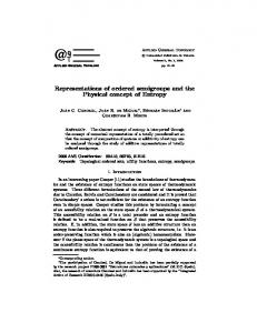
FIG. 10. The same comparisons, with the same labeling as in Fig. 9, using r- I = IOO,Em = l,dt=O.OOS.

t

f

This can be done most simply by replacing the functional integral over e ± iG, which we call (e ± iG), by the quantity [I (e ± iG) 12] 1/2, a computation we henceforth label "renormalized." More general, non-WNG weightings may be treated by calculating Gaussian fluctuations with correlation function given by ll.ij (tl - t 2 )

=

(Ei (tl )Ej (t2»

= oij (EmI2r)e -1/\ -

t211r,

where r is a correlation time, and Em an appropriate magnitude. The limit r- I --+ 00 for Em = 1 is the WNG case, ll.ij --+OijO(t1 - t2 ), while the opposite limit, r-I--+O is effectively the adiabatic limit. (This last remark would be)trictly trueifp were defined as IdEldt liE 2rather than as IdE Idt II E; in practice there seems to be little difference.) We illustrate in Figs. 9 and 10 calculations in the WNG region (r- I = 100) over a variety of different possible approximations, and note that here the best agreement with the exact functional integration is given by first performing the large-p approximation of 5, 5( p) -lip, and then performing the functional integration. Why this is true-rather than using the exact 5( p) and letting the natural, large-p fluctuations automatically induce the effective large-p form of is a reflection of the comments made at the end of Sec. III. In the numerical computations there are many su~cessive choices of Ei that correspond to large variations of E, but of small magnitude, superimposed on a perpendicular component oflarge magnitude and slow variation; and these fluctuations are to be interpreted as adiabatic contributions of small, effective p. When the full5( p) is used, such small-p contributions are incorrectly taken into account. However, with the large-p form of5,5 - lip, the corresponding contributions to (tr U) are small for small p, since such exponentiated terms are rapidly damped away. Using the large-p form of 5( p) suppresses such incorrect, effectively small-p behavior; and, as one can see from Figs. 9 and 10, provides fairly reasonable approximations to the exact result.

s-

23

J. Math. Phys., Vol. 28, No.1, January 1987

v. THREE-DIMENSIONAL INPUT We here consider the generalization of the material of Sec. III to three-dimensional input E(t), which requires a generalization to time-dependentp. It will be appropriate to comment, firstly, on the derivation given in that section for a time-dependent p, and then to extend the analysis to three dimensions. The passage from the exact equations (3.9)-(3.11) to our approximate, "averaged" forms was performed assuming a constant p, and using the "experimental" properties that J and sin ¢ are given by rapid oscillations superimposed upon a constant background. If p = P (t), one must first determine if the same properties of "averaged" constancy of J and sin ¢ still exist, before an analysis of the same type can be given. The experimental answer, obtained for a variety of choices of the t dependence of p (but always insisting on p ~ 1) is that the angular integrations represented, e.g., by Fig. 11, are only slightly modified; experimentally, J and sin ¢ may still be represented as constant quantities on which are superimposed rapid oscillations. This being the case, it does make sense to apply the same form of argument as was used to arrive at (3.12); but the form of (3.13) will now be complicated by the appearance of an extra term proportional to

+K

as]

cot G. p ap The result is that (3.13) and (3.15) no longer yield an algebraic equation for 5(p), but rather, with specific input dpl dt, a differential equation for 5(p). The complication is decidedly nontrivial. Fortunately, if 5 still falls off as p increases, for p ~ 1 these terms should not have any important effect. More precisely, even if a time-dependent p (but, always, p ~ 1) adds small and rapid oscillations to our "averaged" forms, which need not agree with the small and rapid oscillations of the numerically integrated functions, the slowly varying behavior of the "averaged" forms still reprodp [ (1 - 52) dt p2

M. E. Brachet and H. M. Fried

23


(a)

(b)

/

I

(b) (c)

FIG. 11. Graphs of (a) sin.p, (b) Fo, and (c) J = cos.p cos 8; for E = 10, + 30Icos(6Ot) I.

p(t) = 30

duces that of the exact solutions. This can be clearly seen, even after the "fine-tuning" of Sec. VI, in Fig. 12, where anw containing rapid oscillations inserted into our essentially constant (or slowly varyinbg) w-analysis produces a curve whose small and rapid oscillations do not match the exact ones, but whose "averaged" shape continues to reproduce that of the exact curves. We emphasize that we have not attempted a careful study of this quite complicated point; but we are convinced that, for p ~ 1, the specifically time-dependent effects ofpare not important in developing the "averaged" forms in any way other than the elementary generalizations we have made, UJt-+

f

dt' w(t '),

G = 7S(p)

-+

f

24

with fJ(O)

dt' E(t ')S(p(t '»),

={ulifl+U2if2+U3[E3-

~])v,


(5.1)

= 0,

V(O)

Fo, and

(b) F3 and F3; for

(j)

= 60,

g" 2 =.E2

= 1, and

+ E2 sin fJ,

(5.2a)

cos fJ - EI sin fJ.

(5.2b)

if I =.EI cos fJ

If choose !fJ(t) = S~dt' E 3(t '), then the problem has been reduced to one of two-dimensional input. Writing the exact solutions for Vin the form V = Yo + ieT'Y, and comparing U = Fo + iCT'F with the solution obtained from U = exp [ ju3 ( fJ 12)] V, one has the exact statements (5.3a) Fo = Yo cos(fJ 12) - Y 3 sin (fJ 12), (5.3b) F3 = Yo sin(fJ 12) + Y 3 cos(fJ 12),

F,

in writing our finalformulas (3.17)-(3.24). To substantiate this claim, we point to the superimposed curves of Fo and Fo of Figs. 5, 6, 7, and 12 made for a variety of choices of p ( t) , and using only the Fo of (3.17). In treating the problem of three-dimensional input E (t), it is always possible to perform a transformation on the basic equation (1.1) to yield a similar equation for a related quantity in which there appears a two-dimensional input if (1). For, if one defines another unitary quantity V = e - U/2)1J(t)a,. U, where fJ(t) is a function to be determined, then the matrix V will satisfy

a;;

FIG. 12. Superpositions of (a) Foand 20,ET = 10, andEL = 5.

V=

=

Y I cos(fJ 12)

Y

+Y

(5.3c)

2 sin(fJ 12),

Y I sin(fJ 12).

( 5.3d) In order to write approximate, "averaged" expressions for the lhs of equations (5.3), we now apply the technique of Sec. III, writing, e.g., F2 =

2 cos(fJ /2) -

Fo = Yo cos(fJ 12)

-

Y

3 sin(fJ 12),

(5.4)

and similarly for the other lines of (5.3). Here the Yare constructed in terms of a p( g" 1,2) of the two-dimensional prob~m. Clearly~ g" = (g"i g" I = g" 1/g", g" 2 = g" 2/g".

+ g"~)1/2= (Ei

+E~)I/2,

and

The description is simplest using cylindrical coordinates; if we choose EI = ET cos(wt), E2 = ET sin(wt), E3 = EL cos( vt), then g" I = ET cos(wt - fJ), g" 2 = ET sin(wt - fJ). For simplicity, suppose again that EL and E T' as well as wand v, are all constants; then one immediately calculates M. E. Brachet and H. M. Fried

24


(b)

FIG. 13. Fine detail of the curves of Fig. 12, starting from t

=

0.

(5.5)

exhibiting an explicitly time-dependentp, which will be used to calculate the Yo,;. We again insist on the requirement

FIG. 15. Superpositions of 2? It is not difficult to write the leading term of the adiaba-

27


tic approximation for the case of SU (N), but its corrections will surely be more complicated because of the more cumbersome statement of unitarity. 5 In the stochastic limit, on the other hand, the situation seems less well-defined, and the methods of Sec. III would appear to be hazardous and uncertain. In principle, the same techniques can be used; in practice, the greater number of functions Fo,;, 1