Higher-Order Resonances in Dynamical Systems - Core

Higher-Order Resonances in Dynamical Systems

Hogere-orde Resonantie in Dynamische Systemen (met een samenvatting in het Nederlands en Indonesisch)

Proefschrift ter verkrijging van de graad van doctor aan de Universiteit Utrecht op gezag van de Rector Magnificus, Prof. dr. W.H. Gispen, ingevolge het besluit van het College voor Promoties in het openbaar te verdedigen op maandag 25 november 2002 des middags te 14.30 uur

door

Johan Matheus Tuwankotta geboren op 1 december 1970, te Bandung, Indonesië

Promotor: Prof. dr. F. Verhulst Faculteit der Wiskunde en Informatica Universiteit Utrecht

Dit proefschrift werd mede mogelijk gemaakt met financiële steun van de Koninklijke Nederlandse Akademie van Wetenschappen en CICAT (Center for International Cooperation) TU Delft. 2000 Mathematics Subject Classification: 34C15, 34E05, 37M15, 37N10, 65P10, 70H08, 70H33, 70K30. ISBN 90-393-3202-9

Untuk:

Sien Sien

Contents 3 Chapter 0. Introduction 1. Historical background of dynamical systems 2. Motivations and formulation of the problem 3. Mathematical Preliminary 4. Summary of the results 5. Concluding remarks

3 3 4 6 12 16

Bibliography

17

Chapter 1. Symmetry and Resonance in Hamiltonian Systems 1. Introduction 2. Higher order resonance triggered by symmetry 3. Sharp estimate of the resonance domain 4. A potential problem with symmetry 5. The elastic pendulum 6. Conclusion and comments

19 19 20 22 24 31 34

Bibliography

37

Chapter 2. 1. 2. 3. 4. 5.

Geometric Numerical Integration Applied to the Elastic Pendulum at Higher Order Resonance Introduction Symplectic Integration The Elastic Pendulum Numerical Studies on the Elastic Pendulum Discussion

39 39 40 42 44 50

Bibliography

53

Chapter 3. Hamiltonian systems with Widely Separated Frequencies 1. Introduction 2. Mathematical formulation of the problem 3. Domain of bounded solutions 4. Normal form computation 5. First order analysis of the averaged equations 6. Second order averaging if a4 = 0

55 55 57 58 59 61 64

2

Contents 7. 8. 9.

Application of the KAM theorem Application to nonlinear wave equations Concluding remarks

Bibliography Widely Separated Frequencies in Coupled Oscillators with Energy-preserving Quadratic Nonlinearity 1. Introduction 2. Problem formulation and normalization 3. General invariant structures 4. The rescaled system 5. Two manifolds of equilibria 6. Bifurcation analysis of the energy-preserving system 7. The isolated nontrivial equilibrium 8. Hopf bifurcations of the nontrivial equilibrium 9. Numerical continuations of the periodic solution 10. Concluding remarks

66 67 73 75

Chapter 4.

77 77 81 83 84 85 87 93 95 97 102

Bibliography

105

Chapter 5. Heteroclinic behaviour in a singularly perturbed conservative system 1. Introduction 2. Problem formulation 3. On singularly perturbed conservative systems 4. The fast dynamics 5. Nontrivial equilibrium 6. Bifurcation analysis 7. Concluding remarks

107 107 109 110 112 113 114 121

Bibliography

123

Appendix Additional reference to Chapter 1

125 125

Samenvating

127

Ringkasan

129

Acknowledgment

133

About the author

135

CHAPTER 0

Introduction 1. Historical background of dynamical systems Nonlinear Dynamics is a topic of interest in various fields of science and engineering. A lot of problems arising in science and engineering can be modeled as a dynamical system. To name but a few, population dynamics, celestial mechanics, atmospheric models, the prediction of the stock market prices. Among these examples, celestial mechanics is by far the oldest. Already in 1772, Euler described the well-known Three-Body Problem in his attempt to study the motion of the moon. In a more general form, the N -body problem remains a subject of study until now. We refer to [18] for a brief history of the three-body problem and for more references. Some of the recent developments in applications of dynamical systems in Physics, Biology and Economy, are nicely presented in a book by Mosekilde [15]. A revolutionary contribution to the theory of dynamical systems has been made by the French mathematician Henri Poincaré. Before his time, the studies on dynamical systems were concentrated on finding solutions in the sense of explicit functions that solve the equations of motion. Poincaré’s proposal was to look at the geometry of solutions instead of explicit formulas for the solution. As a consequence, in comparison with the classical technique, his technique managed to deal with many more problems. Poincaré invented powerful qualitative methods in order to get hold on the global behavior of the solutions, in situations where the quantitative aspects were out of reach because of lack of explicit formulas or powerful electronic computers in order to compute them. His studies also initiated a new branch of mathematics called Topology. Bifurcation theory is another subject in the theory of dynamical systems which finds its origin in the work of Poincaré. To put it in a simple way, bifurcation theory deals with a parameterized family of dynamical systems and the qualitative variations in the family if we vary the parameters. This topic is without any doubt very important in understanding a dynamical system from the mathematical point of view as well as from the applications. From the point of view of applications, it is important to study a family of dynamical systems to have a complete picture of the system under consideration. Think of a practical problem which involves measurements to determine the parameters of the system. In doing measurements, one cannot have a 100 % precision. Thus, one would have to consider a family of dynamical systems containing the actual problem. From a mathematical point of view, studying one particular dynamical system is like

4

Introduction

analyzing a projection to a two-dimensional plane of a three-dimensional object. One must be very lucky in choosing a right plane out of infinitely many possibilities to be able to recognize the shape of the object. Most of the time, one gets only partial information from such a projection. In the 20th century, the existence of a new phenomenon was acknowledged by the scientific world. Although it has been realized by Poincaré, this new exciting phenomenon called Chaos came into play only around 1960. It originated in models which arose in applications, namely models in solid mechanics (Duffing equation, 1918), electric circuit theory (Van der Pol equation, 1927), atmospheric research (Lorenz equation, 1963) and astrophysics (Hénon-Heiles, 1964). We have to note that the contributions of Van der Pol and Duffing were more in the nonlinear dynamics field. It was only later that people found chaos in their models. In the mathematical world, driven by some of these results, Stephen Smale was forced to admit the existence of chaos which contradicted his own idea of deterministic systems. He reacted positively and in 1963, he constructed the so-called horseshoe map which provides one of the possible ingredients for the onset of chaos in dynamical systems. 2. Motivations and formulation of the problem This thesis is a collection of studies on a particular (but important) family of dynamical systems, namely systems of coupled oscillators. In Section 3 we will describe this family again with more details. Systems of coupled oscillators arise abundantly in applications. The reader could consult a book by Nayfeh and Mook [17] which contains a lot of mechanical examples. Another example, which is still from the field of mechanical engineering, is a book by Tondl et. al. [22]. This book is concentrated on a special class of systems called auto-parametric systems. Systems of coupled oscillators also could be derived from various partial differential equations; for example wave equations [14], or beam equations [4]. Think of a system of two linear undamped oscillators with frequencies ω1 and ω2 . Resonance is the situation where ω1 /ω2 ∈ Q. Solutions of such a system live in twodimensional tori parameterized by the value of the energy of each of the oscillations (except if one of the energies is zero). It is well known that in the case of nonresonance, each torus is densely filled with a solution. In the case of resonance, all solutions are periodic with period of T (which is equal to the smallest common positive integral multiple of 1/ω1 and 1/ω2 ). See [8] for a detailed study on two linear undamped oscillators. If we add nonlinear terms to the system above, a natural question would be whether the geometry of the phase space is changed. There are three things that contribute to the complexity of the analysis. The first is that the frequency of each of the oscillations becomes dependent on its energy due to the presence of the nonlinear terms. Secondly, the nonlinear terms also contain a coupling between the oscillations. Thus, energy can be transferred from one oscillator to the other. Thirdly, in general the solutions will no longer be confined to two-dimensional tori, but wander around in a complicated manner on the three-dimensional hyper-surfaces in the phase space

2 Motivations and formulation of the problem

5

determined by the value of the energy. However, we will see that for small energies the difference with motions on tori is, for bounded time intervals, smaller in order than any power of the energy. Let us consider only weakly nonlinear systems: the order of magnitude of the nonlinear terms is small compared to the linear oscillations, as is the case for small amplitudes. The energy exchanges correspond to a change in the geometrical way in which the phase space is filled up with the two-dimensional tori on which the motion takes place. Recall that if there is no nonlinear term, the solutions live on invariant two-dimensional tori which are the Cartesian product of the two circles of constant energy of each of the oscillators. If there is an energy exchange between the oscillators, the tori must be deformed. In low-order resonances like the 1 : 2 resonance, the measure of these energy exchanges is large. A good example to this phenomenon is a study by Van der Burgh [28] on a classical mechanical example of a two-degrees of freedom Hamiltonian system: the elastic pendulum (also known as spring-pendulum). The elastic pendulum is like an ordinary pendulum except that we replace the rigid bar with a spring. The linearized system consists of two decoupled linear oscillations: the swinging mode (like an ordinary pendulum) and radial oscillation mode due to the spring when the pendulum hangs vertically. The second oscillation is unstable in the case of the 1 : 2 resonance. Thus, a small deviation from the vertical will generate a swinging motion. It means that energy is transferred from the radial oscillation to the swinging mode, and back. The measure of energy which is transferred is of the same order of magnitude as the energy in the system. High-order resonances have received less attention in the literature. One of the reason for this is that the energy exchanges are confined to a small domain in phase space. The measure of energy which is transferred from one mode to the other is small. In this thesis, we concentrate on studying systems of coupled oscillators at high-order resonances. Apart from filling some gaps which have been left open in the classical literature, we also improve some of the known results on high-order resonances in two degrees of freedom Hamiltonian systems. In relation with resonances, we consider also the effect of discrete symmetry such as mirror symmetry and reversing symmetry to a system. The motivation for this is that in nature, such symmetries are abundant. The presence of such symmetries complicates the analysis since it usually leads to certain degeneracies in the equations for the invariant tori. In our analysis, we will be using normal form theory a lot. This leads to a simplification of a finite part of the Taylor expansion of the system at the origin, by means of suitable substitutions of variables. On this simpler system, we perform the analysis to gain as much as possible information about the dynamics. In this way we obtain an asymptotic approximation of the motion of the original system. Sometimes the approximation is accurate enough in order to draw conclusions about exact solutions, such as the existence of families of periodic solutions with not too long periods which are close to the singular fibers of the torus fibration of the normal form.

6

Introduction

The results in this thesis would be interesting in particular from an application point of view. However, we are not working specifically with particular problems from applications. They appear only as examples of our analysis. Our goal is to provide some mathematical insight to a class of dynamical systems which arise quite a lot in applications. We present the analysis and the result in a rather explicit way. We also try to make the connection with applications as clearly as possible. 3. Mathematical Preliminary 3.1. Dynamical systems. Consider a one parameter family of transformations in Rm parameterized by t: Φ = {ϕt |ϕt : U → Rm , U ⊆ Rm }. The following properties hold in Φ: ϕ0 = Im (the identity transformation in Rm ) and ϕt+s = ϕs ◦ ϕt . Dynamical systems consist of these three ingredients: the phase space Rm , time which is denoted by t, and the time evolution law encoded in Φ. If t ∈ R then the system is called continuous dynamical system or flow. If t ∈ Z, it is called discrete dynamical system or map. If ϕt only exist for t ≥ 0, t ∈ R, then they form a so-called semi-flow. This occurs for instance in partial differential equations of diffusion type, and will not be discussed in this thesis. Consider a vector field F : Rm → Rm , and the dynamical system of which the motion is determined by a system of first-order Ordinary Differential Equations (ODEs), i.e. d ξ = ξ˙ = F (ξ), dt where ξ ∈ Rm . A system of first order ODEs is called autonomous if the function F does not depend explicitly on the time variable t. The system of ODEs: ξ˙ = F (ξ) is also called the equations of motion. (0.1)

A point in phase space ξ◦ which is kept invariant under the flow of dynamical system (0.1) is called equilibrium. This point corresponds to a critical point of the vector field: X(ξ ◦ ) = 0. For maps, the point is called fixed point. Another interesting solution is periodic solution: a non-constant solution ξ(t) satisfying: ξ(t + T ) = ξ(t) for a T 6= 0. Let ξ◦ be an equilibrium of system (0.1). A solution ξ(t) 6= ξ ◦ satisfying lim ξ(t) = ξ◦ ,

t→±∞

is called homoclinic orbit. Another object of interest that we will also see in this thesis is a heteroclinic orbit. Let ξ◦ and ξ ◦◦ be two (distinct) equilibria of system (0.1). A heteroclinic orbit is defined as an orbit ξ(t) which is non constant, satisfying lim ξ(t) = ξ ◦ , and

t→+∞

lim ξ(t) = ξ◦◦ .

t→−∞

One would like also to look for an invariant manifold: a manifold M ⊂ Rm such that ϕt (M ) ⊂ M where ϕt is the flow of system (0.1). This invariant manifold might have a special geometry such as invariant sphere or invariant torus.

3 Mathematical Preliminary

7

Stability results for the above mentioned invariant structures are important. Here we use mainly two different stability types: neutrally stable (or Lyapunovstable) and asymptotically stable. In a neutrally stable situation, nearby solutions stay close to the invariant structure as time increases while in an asymptotically stable situation, nearby solutions get attracted. We also have the notion of local (in phase space) stability and global stability. If we vary the parameter in our dynamical system, these invariant structures might undergo a change of stability. This phenomenon is known as bifurcation. Let ϕt be a flow. For a fixed T ∈ R, the map ϕT , the flow after time T is called stroboscopic map. This map is useful in particular when dealing with non-autonomous systems defined by a T -periodic vector field. The initial value for T -periodic solutions of such a system are precisely the fixed points of ϕT , i.e. the points ξ such that ϕT (ξ) = ξ. The long term behavior of the system can be read off from the behavior of the iterates: ϕT n = ϕnT of the stroboscopic map. In autonomous systems, it is more useful to construct a so-called Poincaré section of the flow. This is defined as an (m − 1)-dimensional hyper-surface Σ in Rm , such that the vector field of the system is nowhere tangent to Σ. Let Σ◦ be the set of all ξ ∈ Σ such that ϕt (ξ) ∈ Σ for some t > 0. Let us write T = T (ξ) for the minimal t > 0 such that ϕt (ξ) ∈ Σ. Then, the Poincaré map P : Σ◦ → Σ is defined by P (ξ) = ϕT (ξ) (ξ). It follows from the transversality condition that Σ◦ is an open subset of Σ and T (ξ) and P (ξ) depend smoothly on ξ ∈ Σ◦ . Periodic solutions (of period T (ξ)) correspond to fixed points ξ of P . If one is lucky, then Σ◦ = Σ and one can study all iterates P n , but in general it can happen that P n (ξ) runs off Σ for some (large) n. 3.2. Hamiltonian systems. Consider R2n as a symplectic space with coordin nate form, i.e. dx ∧ dy = Pn ξ = (x, y) where x, y ∈ R and a standard symplectic 1 dx ∧ dy . Let H(ξ) be a real-valued, smooth enough function which is defined j j 1 in R2n . Using H, we can define a Hamiltonian system of ODEs (0.2) ξ˙ = J dH(ξ), where

¶ 0 In . J= −In 0 and In is the n × n identity matrix. This matrix J is also known as a standard symplectic matrix. The function H is called the Hamiltonian function (or just Hamiltonian). The natural number n is called the number of degrees of freedom of the Hamiltonian system. It is an easy computation to show that the orbital derivative of H(ξ) along T the solutions of the Hamiltonian system (0.2), i.e. (dH(ξ)) J dH(ξ) vanishes everywhere. This means that the flow of Hamiltonian system (0.2) is everywhere tangent to the level sets of H, which implies that the function H is kept constant µ

1In this case we need only C 2 -function. For normalization, we need H to be a smoother

function.

8

Introduction

along the solutions of system (0.2). Such a system is called conservative system. In a Hamiltonian system also the Liouville measure is preserved. Pn In some parts of this thesis, we assume that H(ξ) = 1 12 yj 2 + V (x). As a consequence, the Hamiltonian system becomes x˙ i

=

y˙ i

=

yi

∂V , i = 1, . . . , n. ∂xi This class of Hamiltonian systems is also known as potential systems. They arise a lot in problems from mechanical engineering. (0.3)

−

3.3. Systems of coupled oscillators. In this thesis, we study a special family of dynamical systems, namely systems of coupled oscillators. The equations of motion of such dynamical systems are (0.4)

x˙ j y˙ j

= yj = −ωj xj + fj (x, y),

for j = 1, . . . , n, ωj ∈ R+ and x, y ∈ Rn , where n is a natural number. The function ˙ is assumed to be sufficiently smooth. Moreover, we assume that fj (0, 0) = 0 fj (x, x) ∂f and ∂xji (0, 0) = 0, for i, j = 1, . . . , n. The system (0.4) is equivalent to (0.5)

˙ x ¨j + ωj xj = fj (x, x),

for j = 1, . . . , n. 3.4. Bifurcation. Two vector fields on Rn are topologically orbitally equivalent, if there exists a orientation-preserving homeomorphism h : Rn → Rn that maps orbits of the first vector field to orbits of the second vector field in such a way such that no time re-orientation is required. Those two vector fields are said to be conjugate. Let us consider a one-parameter family of dynamical systems, defined by ξ˙ = Xµ (ξ), where ξ ∈ Rn , µ ∈ R, and Xµ is a vector field on Rn for an arbitrary but fixed µ. It is said that the dynamical system ξ˙ = Xµ (ξ), undergoes a bifurcation at µ◦ if the vector fields Xµµ◦ . Another approach to bifurcation theory is using singularity theory, see [9]. One of the central question in this approach is to classify the type of bifurcations, see also [3]. For a more applied mathematics oriented reference, see [13]. 3.5. Normalization. Consider a system of ODEs: ξ˙ = F (ξ) with an equilibrium point at the origin: F (0) = 0 and ξ ∈ Rm . In order to analyze the behavior of the solutions near the origin, it is very useful to construct nonlinear coordinate transformations that bring the system into a simpler form (the meaning of simple is obviously contextual). We can expand F in its Taylor series, i.e. (0.6)

ξ˙ = A ξ +

k X

F j (ξ) + . . . ,

2

where A is a constant matrix and F j , j = 2, . . . , k are homogeneous polynomials of degree j.


9

In the normal form procedure one tries to simplify the higher order terms Fj subsequently for j = 2, 3, etcetera. In order to see what we can do for Fk , let ξ = ζ + Gk (ζ) + . . . where Gk is homogeneous of degree k and the dots denotes a remainder term consists of higher order terms. A nonzero remainder term is sometimes needed, for instance if one requires that the substitution of variables leaves some structure invariant, such as symplectic form or a volume form. Then (Im + dG(ζ) + . . .)ζ˙ = ξ˙ = A (ζ + G(ζ)) +

k X

F j (ζ + G(ζ)) + . . . ,

2

where the dots in the righthand side vanish of order k + 1. Note that for small k ζ k the inverse of Im + dGk (ζ) + . . . exists and is equal to Im − dGk (ζ) + . . ., where the dots indicates terms which vanish of order k. It follows that (0.7)

ζ˙ = A ζ +

k X

F j (ζ) + (A Gk (ζ) − dGk (ζ) A ζ) + . . . ,

2

where the dots vanish of order k + 1. This means that the substitution leads to an addition of the k-th order term (ad A) (Gk ) := AGk (ζ) − dGk (ζ)Aζ, which can be recognized as the commutator [A, Gk ] of the linear vector field A with the vector field Gk , to F k (ζ). Let Xk (Rm ) denotes the space of all homogeneous polynomial vector fields of degree k in Rm . Then Xk (Rm ) is a finite-dimensional vector space and (0.8)

Ad A

: :

Xk (Rm ) −→ Xk (Rm ) X 7−→ AXA−1 ,

defines a linear mapping in Xk (Rm ), if A is invertible. The infinitesimal version of this mapping is ad A. If the linear mapping Ad A is complex-diagonalizable (or also known as semi-simple) then ad A is also complex-diagonalizable, which in turn implies that Xk (Rm ) = im(ad A) + ker(ad A). As a conclusion, with the normal form procedure at order k one can arrange that the transformed k-th order term F k = F k + (ad A)(Gk ) to be in the ker(ad A): (ad A)(F k ) = 0, which means that F k commutes with the linear vector field A. This is done by splitting F k into F˜k + Fˆk , where F˜k ∈ im(ad A) and Fˆk ∈ ker(ad A). Thus, we have to solve (ad A)(Gk ) = −F˜k . In this way one can subsequently arrange that all the terms of the Taylor expansion of F up to any desired order commute with A. This result is known in the literature as the Birkhoff-Gustavson normal form at an equilibrium point of a vector field. For Hamiltonian systems, instead of normalizing the Hamiltonian vector field, we can normalize the Hamiltonian itself. This is easier since we are working in an algebra of real-valued functions. Recall that our symplectic space is R2n with symplectic form: dx ∧ dy. Let Pk be the space of homogeneous polynomials of degree k in the

10

Introduction

canonical L variables (x, y). The space of all (formal) power series without linear part, P ⊂ k≥2 Pk , is a Lie-algebra with the Poisson bracket ¶ n µ X ∂f ∂g ∂f ∂g − . {f, g} = dx ∧ dy(Xf , Xg ) = ∂xj ∂yj ∂yj ∂xj 1 For each h ∈ P , its adjoint ad h : P → P is the linear operator defined by (ad h)(H) = {h, H}. Note that whenever h ∈ Pk , then (ad h) : Pl → Pk+l−2 and (ad h)(H) = −(ad H)(h). Let us take an h ∈ P . It can be shown that for this h there is an open neighborhood U of the origin such that for every |t| ≤ 1 each time-t flow etXh : U → R2n of the Hamiltonian vector field Xh induced by h is a symplectic ¡ ¢∗diffeomorphism on its image. These time-t flows define a family of mappings etXh : P → P by sending ¡ ¢∗ ¡ ¢∗ H ∈ P to etXh H = H ◦ etXh . Differentiating the curve t 7→ etXh H with ¡ ¢∗ d respect to t we find that it satisfies the linear differential equation dt etXh H = ¡ 0X ¢∗ dH · Xh = −(ad h)(H) with initial condition e h H = H. The solution reads ¡ tX ¢∗ e h H = e−t(ad h) H. In particular the symplectic transformation e−Xh transforms H into ¢∗ ¡ 1 (0.9) H 0 := e−Xh H = e(ad h) H = H + {h, H} + {h, {h, H}} + . . . . 2! L −Xh The diffeomorphism e sends 0 to 0 (because Xh (0) = 0). If h ∈ k≥3 Pk , then De−Xh (0) = Id. A diffeomorphism with these two properties is called a near-identity transformation. The next step is identical with the non-Hamiltonian case. We expand equation (0.9) into its Taylor series and normalize degree by degree. The homology equation that we need to solve in each step of the normalization is identical, i.e. (ad H2 ) (h) = Hj . The resulting normal form for the Hamiltonian truncated up to degree k, is (0.10)

H = H2 + H 3 + . . . + H k ,

where {H2 , Hk } = 0. But this implies {H2 , H} = 0. Note that {H2 , H} = LXH (H2 ): the orbital derivative of the function H2 along the solutions of Hamiltonian system of ODEs defined by H. Thus, apart from the Hamiltonian function: H, normalization adds to the truncated system an extra constant of motion: H2 . In two degrees of freedom systems, this is enough for integrability of the normal form. Remark 0.1. Near-identity transformations defining the coordinate transformation in Hamiltonian systems, are defined using the flow of a Hamiltonian h. This transformation then, is naturally symplectic (it preserves the symplectic structure). In the non-Hamiltonian case, we need not worry about this. In both cases, if the dynamical system enjoys an additional discrete symmetry, it can be preserved during normalization. 3.6. Resonance. Recall that the terms in the normal form of a vector field are elements of ker(ad A). Thus, it boils down to characterizing the generators of ker(ad A). Let Gα (ζ) = ζ α ej , ej is the standard j-th basis of Rm , and A =


11

diag(λ1 , . . . , λm ), λj ∈ C, j = 1, . . . , m, it is an easy exercise to show that Ã ! m X α (ad A)(ζ ) = λj − αj λj ζ α ej ∈ ker (ad A) 1

Pm if and only if (λj − 1 αj λj ) = 0. This situation is also called resonance and the terms in the normal form are called resonant terms. Similarly for a Hamiltonian system, would like to ¡ ¢ characterize the generators of ker(ad H2 ). Let us assume Pwe n H2 = 1 ωj xj 2 + yj 2 . For computational reason, we transform the variables by uj = xj + iyj and vj = xj − iyj , j = 1, . . . , n. In these new variables, a monomial uα v β is in ker(ad H2 ) if and only if n X (αj − βj ) ωj = 0, 1

which is the resonance condition for Hamiltonian systems. Consider a resonance relation: k1 ω1 + k2 ω2 + . . . + kn ωn = 0,

Pn for a nonzero k = (k1 , k2 , . . . , kn )T ∈ Zn . A number |k| = 1 |ki | is usually used to classify the resonances. A phrase like low-order (or strong, or genuine) resonance, is used to do the classification. From the normal form point of view, the number |k| also corresponds to the degree of the resonant term appearing in the normal form. Resonances are responsible for producing a nontrivial dynamics in the normal form. As a consequence, the higher the resonance is, the higher we have to normalize in order to get nontrivial dynamics. 3.7. Averaging method. In the case of time-periodic vector fields, the normalization described above can also be done using averaging. Let 0 ≤ ε ¿ 1, and consider a system of first-order ODEs (0.11) ξ˙ = εF (ξ, t, ε), where ξ ∈ Rm and there exists T ∈ R such that F (ξ, t + T, ε) = F (ξ, t, ε) for all t. A system of the form (0.11) is also said to be in the Lagrange standard form. Using transformation ξ = ζ + εu(ζ, t) where Zt

1 (F (ζ, s) − F (ζ)) ds and F (ζ) = T ◦

u(ζ, t) = 0

ZT

◦

F (ζ, t)dt, 0

we transform system (0.11) into (0.12) ζ˙ = εF ◦ (ζ) + O(ε2 ). Under some conditions on the function F , if ξ(t) is a solution of system (0.11) and ζ(t) is a solution of system (0.12) with the property: ξ(0) = ζ(0) = ξ◦ ∈ Rm , then ξ(t) − ζ(t) = O(ε) on the time-scale of 1/ε. See [20] for details on the averaging method and the relation with normal forms. For a system of undamped coupled oscillators: ξ˙ = F (ξ), the small parameter ε

12

Introduction

is introduced into the equations by employing a blow-up transformation (or scaling): ξ 7→ εξ. This bring the system (after expanding to its Taylor series) into ξ˙ = A ξ + εF 2 (ξ) + O(ε2 ), where A is a matrix with purely imaginary eigenvalues. The next step: using time-dependent coordinate transformation: ξ = φ(t)ζ where d φ(t) = A φ(t), we bring the system into the Lagrange φ(t) is a matrix satisfying dt standard form. In this standard form, we have a time-periodic vector field (because all nontrivial solutions of ξ˙ = A ξ are periodic). Averaging can also be done while preserving the symplectic structure. 3.8. Additional notes to references. A concise description, using modern mathematics, of the theory of dynamical systems can be found in [12]. A mathematically rigorous approach to dynamical systems can also be found in [1]. For more practically oriented references, see for instance [10, 29]. In [11], recent developments in dynamical systems are nicely presented. In [1], the theory of Hamiltonian systems is treated in a very general manner. Another good reference for the theory of Mechanics can be found in [2]. The theory of normal forms can be found in various standard textbooks on dynamical systems such as [29]. For the theory of normal forms in Hamiltonian systems, we refer to [1, 2, 18, 20]. In [1, 18] normalization using Lie-series method is described. In [2, 20], it is done using averaging and also using generating functions. See also [16] for general perturbation methods in dynamical systems. 4. Summary of the results 4.1. Symmetry and resonance in Hamiltonian systems. We start with considering a two degrees of freedom Hamiltonian system around an elliptic equilibrium. Such a system can be seen as a Hamiltonian perturbation of two linear harmonic oscillators. We assume that the Hamiltonian enjoys a mirror symmetry in one of the degrees of freedom. Using averaging, we construct an approximation for the Hamiltonian system and study its dynamics. Discrete symmetries, such as mirror symmetry or time reversal symmetry, arise naturally in applications. These symmetries receive less attention in the classical literature since they do not correspond to the existence of integrals of motion of the system. However, the presence of these symmetries is quite often responsible for certain degeneracies in the normal form. In [19], J.A. Sanders described the dynamics of two degrees of freedom Hamiltonian systems at higher order resonance defined by Hamiltonian H, with quadratic part ¡ ¢ ¡ ¢ H2 = 12 ω1 x1 2 + y1 2 + 21 ω2 x2 2 + y2 2 , where ξ = (x, y) is a pair of canonical coordinates, ω1 and ω2 are both positive, and ω1 /ω2 6= 13 , 12 , 1, 2, 3. Using a blow-up transformation, the small parameter ε is introduced: ξ 7→ εξ. By rescaling time, we can keep the quadratic part of the Hamiltonian invariant under the blow-up transformation. For a fixed energy, a large part of the phase space (near the origin) of such systems is foliated by¡ invariant¢two-tori parameterized by taking the linear energy of each oscillator: 21 ωj xj 2 + yj 2 , j = 1, 2, to be constant. On these two-dimensional

4 Summary of the results

13

tori, the solutions are conditionally periodic. This can be seen from the fact that in the normal form, the linear energy of each oscillator is constant up to at least quartic terms (that is if we truncate the normal form after the quartic terms). In fact, for most of the initial conditions, these linear energies are constant up to any finite degree of normal form approximation. For those initial conditions, there is no energy exchange between the oscillators. There exists also a domain in phase space where something else happens. In this domain, there is energy exchange, and generically one would find two periodic solutions: one stable and the other is of the saddle type. In fact, one would find more periodic solutions with much higher period. This domain is called the resonance domain. Using the normal form theory, we construct an approximate Poincaré section for the system. By doing this, we have significantly improved the estimate of the size of the resonance domain which is given by Sanders in [19]. We also show, how some of the low-order resonances, such as the 1 : 2-resonance, behave as a higher order resonance in the presence of a particular mirror symmetry. We note that one could preserve the mirror symmetries while normalizing. The kernel of the adjoint operator (0.8) becomes smaller in the presence of some of these symmetries. Since the terms in the normal form are elements of the kernel of the adjoint operator, this means the normal form might have certain degeneracies. This theory is then applied to a classical mechanical system: the elastic pendulum. To our knowledge, Van der Burgh [28] is one of the first who studied this example for the 2 : 1-resonance by using normalization. Following [28], we modeled the elastic pendulum as a two degrees of freedom Hamiltonian system. It enjoys a mirror symmetry in one of the degrees of freedom. The theory produces a new hierarchy of resonances ordered by the lowest degree in the Taylor series of the normal form in which the resonant interaction term appears. For two among the six most prominent resonances, we numerically check the new estimate of the resonance domain we have derived. The numerics shows a good agreement with the theory. This is all presented in the paper [25] and Chapter 1.

4.2. Geometric numerical integration applied to the elastic pendulum at higher order resonance. The characteristic time-scale of the interaction between the degrees of freedom for a Hamiltonian system at high-order resonance is rather long. This is actually the reason why in Chapter 1, we managed to provide numerical confirmation to our estimate, only for two resonances. In Chapter 2, we apply Geometric Numerical Integration to the elastic pendulum at high-order resonance. The integrator that we use is based on the so-called splitting method. The idea is to split the Hamiltonian into several parts for which solutions can be obtained analytically. Using these analytic flows, we construct an approximation for the original flow. An excellent agreement between the theory and numerics is achieved. The idea of using the splitting method is well-known. The goal of the paper [24] is to find a numerical confirmation of the theory that is developed in [25]. We note that the first evidence that the estimate given by Sanders can be improved, is

14

Introduction

found numerically by van den Broek [27]. This is why we would like to achieve a numerical confirmation of the estimate in [25]. The estimate for the size of the resonance domain, is given by using a small parameter ε. This small parameter is explicitly introduced into the equations that we numerically integrate (using the blow-up transformation). Usually, one needs not introduce the small parameter explicitly, but uses a small value of the energy instead. In our case, it is crucial to have this explicit dependency of the vector field on the small parameter. By doing this, we can explicitly vary the small parameter and study the effect of it on the size of the resonance domain. The Hamiltonian in our case is split into three parts. One of these is the quadratic part of the Hamiltonian. By doing this, our numerics preserve the linear structures of the system, such as the linear resonances. The results in this chapter are also presented in [24]. 4.3. Widely separated frequencies in Hamiltonian systems. The next problem that we consider in this thesis is a Hamiltonian system with widely separated frequencies (an example is given below). This can be viewed as an extreme type of high-order resonance. It is only recently (starting around 1990) that people have started to pay some attention to this type of resonances. We present the study on this system in Chapter 3. In [5, 6], Broer et al. described this problem as a two degrees of freedom Hamiltonian system near an equilibrium having a pair of purely imaginary and double zero eigenvalues. Using singularity theory and normal form theory, the unfolding of the equilibrium of such a system is studied. Motivated by this, in Chapter 3, we present a study on the dynamics of such a system, using normal form theory. The normal form is computed explicitly which then can be considered as a supplement to the results in [5, 6]. As in nature discrete symmetries occur quite often, in some cases the normal form is degenerate. We characterize which symmetry causes this to occur and then also compute the higher order normal form. We compare this analysis with that for an ordinary higher-order resonance. We find no energy exchange between the degrees of freedom. However, there is phase interaction on a time-scale which is shorter than in an ordinary high-order resonance. We also distinguish two different ways of having these extreme type of high-order resonances in applications. Think of two systems in which a small parameter ε has been introduced. The first system has a frequencies pair (ω1 , ω2 ) = (1, ε) and the other has a frequencies pair: (ω1 , ω2 ) = ((1/ε), 1). Do they behave in the same way? It turns out that the second system is simpler than the first one. We also consider an application in wave equations. Using Galerkin truncation, one would derive a system of coupled oscillators as an approximation for the wave equation. We consider several possibilities: dispersive and non-dispersive wave equations, and also two types of nonlinearities. The results in this chapter are also presented in [26]. 4.4. Widely separated frequencies in coupled oscillators with energypreserving quadratic nonlinearity. In Chapter 4 we consider a slightly more general system of coupled oscillators. The system is non-Hamiltonian with weak dissipation or weak energy input (or a combination of the two). The nonlinearity

4 Summary of the results

15

is assumed to be quadratic and energy preserving. Thus, the system is a linearly perturbed conservative system. As in the previous chapter, we are interested in the internal dynamics of the system. Therefore, the system in Chapter 4 is also autonomous. Apart from the fact that studies of internal dynamics of such a system are lacking in the literature, we are motivated by a study from the applications in atmospheric research in [7]. The model considered in [7] is derived from the NavierStokes equation projected to a ten-dimensional space. There is a lot of interesting dynamics such as homoclinic behavior, regime transitions etc. which are observed. Two among five modes which are considered, have a high frequency ratio: 12.4163 . . .. Based on this, we set up a system of coupled oscillators having widely separated frequencies and energy-preserving nonlinearity. By doing this, we might be able to provide an alternative explanation for the presence of some of the interesting dynamics. We use normal form theory to construct an approximation for our system. This normal form is computed by averaging out the fast oscillation. The resulting normal form is then reduced to a three-dimensional system of first-order differential equations. Due to the wide separation in the frequencies, we can prove the existence of a manifold which is invariant under the flow of the normal form. Moreover, this manifold can not be perturbed away by adding higher order terms in the normal form. Next, we use the assumption that the nonlinearity preserves the energy. We note that this assumption can be preserved while normalizing. In fact, we split the reduced normal form into the energy-preserving part and the rest. Furthermore, we assume that the rest is small. This boils down to rescaling two of the parameters in the system using a small parameter. The dynamics of the rescaled normal form consists of slow-fast dynamics. The fast dynamics corresponds to the motion on the energy manifolds, which are twodimensional spheres, while the slow dynamics is the motion from one energy manifold to another along the direction of the curves consisting of attracting equilibria of the fast system. Due to non-compactness, we cannot prove the existence of an invariant slow manifold. The dynamics however, is similar: the slow motion is funneling into a very narrow tube along the curve. On this rescaled normal form, we study the bifurcation of the nontrivial equilibrium (analytically) and also the bifurcation of the periodic solution (numerically). This result is used to understand the global behavior of the normal form. In the neighborhood of the trivial equilibrium, for an open set of the parameter values, we find a lot of periodic solutions (most of them are unstable) with high periods. We do not find an orbit which is homoclinic to the nontrivial critical point. This statement is valid up to any finite-degree of the normal form. We do, however, find a finite sequence of period-doubling bifurcations and fold bifurcations which usually is connected to the appearance of a homoclinic orbit. In contrast with the Hamiltonian case in the previous chapter, energy exchanges between the degrees of freedom occur significantly. This is again another counter example to the traditional wisdom in engineering on high-order resonances. It is

16

Introduction

even more severe since we include no forcing term in our model. The results in this chapter are also presented in [23]. 4.5. Heteroclinic behavior in a singularly perturbed conservative system. Chapter 5 is a continuation of the work in Chapter 4. We want to note that some of the results which are presented in this chapter are preliminary. In this chapter, we look at the system which is also studied in Chapter 4, as a singularly perturbed conservative system. The conserved quantity is the energy which is represented by the distance to the origin. We present also a generalization of this idea. Apart from extending the phase space to Rn , we generalize the conserved quantity to any sufficiently smooth function which is critical at zero, has no linear term and has semi-definite quadratic terms. For such a system, we derive a condition for the existence of a nontrivial equilibrium. As is mentioned in the previous chapter, we find curves of equilibria of the fast system. One of these curves, is characterized by a quadratic equation in two variables. We find three possibilities: the equation gives us an ellipse, a hyperbola or a parabola. The first possibility is analyzed in Chapter 4. In this chapter we concentrate on the situation where the curve is a hyperbola. Instead of having a homoclinic-like behavior, in this case we find a heteroclinic-like behavior. It is also interesting to note that there exists a manifold in the parameter space where we have only one equilibrium. This equilibrium is of the saddle type. Also in that manifold we find an attractor which has the shape of a heteroclinic cycle between two saddle points. This attractor is not periodic, nor quasi-periodic, and it has one positive Lyapunov exponent. Thus the system is chaotic. The strange attractor that we find exists in a large open set of parameter values. The size of the attractor (measured by the Kaplan-Yorke dimension dKY ) varies between two and three: 2 < dKY < 3. For some values of the parameters we also find a strange repellor. There is strong evidence that this strange repellor produces a fractal boundary between the basin of attraction of the co-existing stable invariant structures (one of them is the strange attractor). We end this chapter by formulating some open questions that arose during the execution of this research. We present these as subjects for further investigation. 5. Concluding remarks In this thesis, we present a study of high-order resonances in dynamical systems. Going through chapter by chapter, one would find an interplay between analytical and numerical work. We present the analytical work as explicitly as possible, although we try to avoid presenting the explicit calculation. This thesis is a collection of research papers, each chapter can be read separately. We hope that it is enjoyable to read this work as much as we have enjoyed the work.

Bibliography [1] Abraham, R., Marsden, J.E., Foundations of Mechanics. The Benjamin/Cummings Publ. Co., Reading, Mass., 1987. [2] Arnol’d, V.I., Mathematical Methods of Classical Mechanics, Springer-Verlag, New York etc., 1978. [3] Arnold, V.I., Geometrical Methods in the Theory of Ordinary Differential Equations, SpringerVerlag, New York etc., 1983. [4] Boertjens, G.J., van Horssen, W.T., An Asymptotic Theory for a Beam Equations with a Quadratic Perturbation, SIAM J. Appl. Math., vol. 60, pp. 602-632, 2000. [5] Broer, H.W., Chow, S.N., Kim, Y., Vegter, G., A normally elliptic Hamiltonian bifurcation, ZAMP 44, pp. 389-432, 1993. [6] Broer, H.W., Chow, S.N., Kim, Y., Vegter, G., The Hamiltonian Double-Zero Eigenvalue, Fields Institute Communications, vol. 4, pp. 1-19, 1995. [7] Crommelin, D.T.Homoclinic Dynamics: A Scenario for Atmospheric Ultralow-Frequency Variability, Journal of the Atmospheric Sciences, Vol. 59, No. 9, pp. 1533-1549, 2002. [8] Cushman, R.H., Bates, L. M.,Global aspects of classical integrable systems, Birkh¨ auser Verlag, Basel, 1997 [9] Golubitsky, M., Schaeffer, D.G., Singularities and Groups in Bifurcation Theory, vol. 1, Applied Math. Sciences 51, Springer-Verlag, 1984. [10] Guckenheimer, J., Holmes, P., Nonlinear Oscillations, Dynamical Systems, and Bifurcations of Vector Fields, Applied Math. Sciences 42, Springer-Verlag, New York etc., 1983. [11] Haller, G., Chaos Near Resonance, Applied Math. Sciences 138, Springer-Verlag, New York etc., 1999. [12] Katok, A., Hasselblatt, B., Introduction to the modern theory of dynamical systems, with a supplementary chapter by Katok and Leonardo Mendoza, Encyclopedia of Mathematics and its Applications, 54. Cambridge University Press, Cambridge, 1995. [13] Kuznetsov, Yuri A., Elements of applied bifurcation theory, second edition, Applied Mathematical Sciences, 112. Springer-Verlag, New York, 1998. [14] Landa, P.S., Nonlinear Oscillations and Waves in Dynamical Systems, Mathematics and Its Application, vol. 360, Kluwer Academic Publisher, Dordrecht etc., 1996. [15] Mosekilde, Erik, Topics in Nonlinear Dynamics. Applications to Physics, Biology, and Economic systems, World Scientific, 1996, Singapore. [16] Murdock, J. A., Perturbations. Theory and methods, Corrected reprint of the 1991 original, Classics in Applied Mathematics, 27. Society for Industrial and Applied Mathematics (SIAM), Philadelphia, PA, 1999. [17] Nayfeh, A.H., Mook, D.T., Nonlinear Oscillations, Wiley-Interscience, New York, 1979. [18] Rink, B., Tuwankotta, T.,Stability in Hamiltonian Systems: Applications to the Restricted Three Body Problem., to appear in the proceedings of the Mechanics and Symmetry, Euro Summer School, Peyresq, September 2000. [Online] http://www.math.uu.nl/publications/preprints/1166.ps.gz. [19] Sanders, J.A.,Are higher order resonances really interesting?, Celestial Mech. 16, pp. 421-440, 1978.

18

Bibliography

[20] Sanders, J.A., Verhulst, F., Averaging Method on Nonlinear Dynamical System, Applied Math. Sciences 59, Springer-Verlag, New York etc., 1985. [21] Shidlovskaya, E.G., Schimansky-Geier L., Romanovsky, Yu. M., Nonlinear Vibrations in a 2Dimensional Protein Cluster Model with Linear Bonds, Zeitschrift f¨ ur Physikalische Chemie, Bd. 214, H. 1, S. 65-82, 2000. [22] A. Tondl, M. Ruijgrok, F. Verhulst, and R. Nabergoj, Autoparametric Resonance in Mechanical Systems, Cambridge University Press, New York, 2000. [23] Tuwankotta, J.M., Widely Separated Frequencies in Coupled Oscillators with Energypreserving Quadratic Nonlinearity, preprint Universiteit Utrecht 1245, 2002. [Online] http://www.math.uu.nl/publications/preprints/1245.ps.gz. [24] Tuwankotta, J.M., Quispel, G.R.W., Geometric Numerical Integration Applied to the Elastic Pendulum at higher order resonance, accepted for being published in Journal of Computational and Applied Mathematics. [Online] http://www.math.uu.nl/publications/preprints/1153.ps.gz. [25] Tuwankotta, J.M., Verhulst, F., Symmetry and Resonance in Hamiltonian System, SIAM J. Appl. Math, vol 61 number 4, pp. 1369-1385, 2000. [26] Tuwankotta, J.M., Verhulst, F., Hamiltonian systems with widely separated frequencies, preprint Universiteit Utrecht 1211, 2001 [Online] http://www.math.uu.nl/publications/preprints/1211.ps.gz. [27] van den Broek, B., Studies in Nonlinear Resonance, Applications of Averaging, Ph.D. Thesis University of Utrecht, 1988. [28] van der Burgh, A.H.P., On The Higher Order Asymptotic Approximations for the Solutions of the Equations of Motion of an Elastic Pendulum, Journal of Sound and Vibration 42, pp. 463-475, 1975. [29] Wiggins, S., Introduction to Applied Nonlinear Dynamical Systems and Chaos, Text in Applied Mathematics 2, Springer Verlag, 1990. [30] Yoshida, H., Construction of Higher Order Symplectic Integrators, Phys. Lett. 150A, pp. 262268, 1990.

CHAPTER 1

Symmetry and Resonance in Hamiltonian Systems A joint work with Ferdinand Verhulst Abstract. In this paper we study resonances in two degrees of freedom, autonomous, Hamiltonian systems. Due to the presence of a symmetry condition on one of the degrees of freedom, we show that some of the resonances vanish as lower order resonances. After giving a sharp estimate of the resonance domain, we investigate this order change of resonance in a rather general potential problem with discrete symmetry and consider as an example the H´ enon-Heiles family of Hamiltonians. We also study a classical example of a mechanical system with symmetry, the elastic pendulum, which leads to a natural hierarchy of resonances with the 4 : 1-resonance as the most prominent after the 2 : 1-resonance and which explains why the 3 : 1-resonance is neglected.

Keywords. Hamiltonian mechanics, higher-order resonance, normal forms, symmetry, elastic pendulum. AMS clasification. 34E05, 70H33, 70K30

1. Introduction Symmetries play an essential part in studying the theory and applications of dynamical systems. In the old literature, attention was usually paid to the relation between symmetry and the existence of first integrals but recently the relation between symmetry and resonance, in particular its influence on normal forms has been explored using equivariant bifurcation and singularity theory; see Golubitsky and Stewart [11], Golubitsky et al. [10] or Broer et al. [5] and also [29] for references. For a general dynamical systems reference see [1, 6]; for symmetry in the context of Hamiltonian systems see [6, 15, 28]. In the literature the emphasis is usually on the low-order resonances like 1 : 2 or 1 : 1 for the obvious reason that in these cases there is interesting dynamics while the number of nonlinear terms to be retained in the analysis is minimal. This emphasis is also found in applications, see for instance Nayfeh and Mook [16] for examples of mechanical engineering. As in practice higher-order resonance will occur more often than the low-order case we shall focus here on the theory and application of higher-order resonance, extending [21, 22]. In our analysis we shall use normal forms where in the usual way a small parameter ε is introduced by re-scaling the variables, see section 2. The implication is

20

Symmetry and Resonance in Hamiltonian Systems

that, as ε is small we analyze the dynamics of the Hamiltonian flow in the neighborhood of equilibrium corresponding with the origin of phase-space. Note that ε2 is a measure for the energy with respect to equilibrium. Putting ε = 0, the equations of motion reduce to linear decoupled oscillators. Apart from considering frequency ratios one can also classify resonance in the sense of energy interchange between the degrees of freedom. Terms like strong (or genuine) resonance and weak resonance are used to express the order of energy interchange on a certain time-scale which is characteristic for the dynamics of the system; see the discussion in section 6. Symmetries arise naturally in applications, think for instance of the plane of symmetry of a pendulum or, on a much larger scale, the three planes of symmetry of an elliptical galaxy; an introduction and references are given in [29]. In section 2 we present the framework of our analysis by indicating how symmetry assumptions affect resonance and the normal forms. We use Birkhoff-Gustavson normalization which is equivalent with averaging techniques. In section 3 we give a new sharp estimate of the size of the resonance domain at higher order resonance. Section 4 focuses on a special resonance, the 1 : 2-resonance for symmetric potential problems; we discuss an example from an important family of potential problems for which applications abound. The classical example is the Hénon-Heiles problem [12] which applies to axisymmetric galaxies but also to nonlinear chains as in the Fermi-Pasta-Ulam problem, see [8]. Molecular dynamics uses such twodegrees-of-freedom formulations, for instance in [17, 24]. In mechanical engineering many examples can be found in [16], see also the treatment of the spring-pendulum in [5]. Section 5 discusses one of the classical mechanical examples with symmetry, the elastic pendulum. This system has played a part in applications in aeronautical engineering [9, 20], celestial mechanics [18], astrophysics and aeronautics [13, 14, 18] and biology [2, 19]. In this problem, we show that the symmetry assumption produces a new hierarchy of resonances in which, after the well-known 2 : 1-resonance, the 4 : 1-resonance is the most prominent one. The asymptotic analysis is supplemented by numerical calculations which show excellent agreement. 2. Higher order resonance triggered by symmetry Consider a two degrees of freedom Hamiltonian ¡ ¢ ¡ ¢ (1.1) H(q, p) = 12 ω1 p1 2 + q1 2 + 21 ω2 p2 2 + q2 2 + H3 + H4 + · · · . with (q, p) = (q1 , q2 , p1 , p2 ), Hk , k ≥ 3, a homogeneous polynomial of degree k. We introduce a small parameter ε into the system by rescaling the variables by qj = εqj , pj = εpj , j = 1, 2 and divide the Hamiltonian by ε2 . We can define successive nonlinear coordinate (or near-identity) transformations that will bring the Hamiltonian into the so-called Birkhoff normal form. In action-angle variables, a Hamiltonian H is said to be in Birkhoff normal form of degree 2k if it can be written as H = ω1 τ1 + ω2 τ2 + ε2 P2 (τ1 , τ2 ) + ε4 P3 (τ1 , τ2 ) + · · · + ε2k−2 Pk (τ1 , τ2 ),

2 Higher order resonance triggered by symmetry

21

where Pi (τ1 , τ2 ) is a homogeneous polynomial of degree i in τj = 12 (pj 2 +qj 2 ), j = 1, 2. The variables τ1 , τ2 are called actions; note that if Birkhoff normalization is possible, the angles have been eliminated. If a Hamiltonian can be transformed into Birkhoff normal form, the dynamics is fairly regular. The system is integrable with integral manifolds which are tori described by taking τ1 , τ2 constant. The flow on the tori is quasi-periodic. In normalizing, it is convenient if we transform to complex coordinates by xj yj

= =

qj + ipj qj − ipj , j = 1, 2,

˜ = 2iH. The idea of Birkhoff-Gustavson norwith corresponding Hamiltonian H malization is to transform H (we have dropped the tilde) so that the transformed Hamiltonian becomes (1.2)

H(x, y) = Bk (τ1 , τ2 , ε) + R(x, y, ε)

where (x, y) = (x1 , x2 , y1 , y2 ) Bk is in Birkhoff normal form with k as high as possible (τj = 21 xj yj , j = 1, 2). R is a polynomial which has degree of either 2k or 2k + 1 in (x, y). The terms R are also known as resonant interaction terms and H in this form is called the Birkhoff-Gustavson or resonant normal form. In this paper we will refer to the terms in R as resonant terms. For normalization one can use a generating function or suitable averaging techniques. See for example [1] appendix 7 or [28] chapter 11. The presence of resonant terms of the lowest degree in the Hamiltonian determines until what order the normalization should be carried out. For example, consider the Hamiltonian (1.1) and assume there is a pair of natural numbers (m, n) such that m/n = ω1 /ω2 where m and n are relatively prime. The resonant terms of the lowest degree are generally found in Hm+n ; ω1 : ω2 is said to be a lower order resonance if the corresponding resonant terms of the lowest degree are found in Hk with k < 5. If m + n ≥ 5 the normal form (1.2) becomes (1.3)

H(x, y) = 2i(Bk (τ1 , τ2 , ε) + εm+n−2 (Dx1 n y2 m + Dy1 n x2 m )) + · · · .

It turns out that some of the lower order resonances are eliminated by symmetry in which case m and n need not be relative prime. This is due to the fact that during normalization symmetries can be preserved. See for example [7]. In table 1 we present a list of lower order resonances and its corresponding resonant terms of the lowest degree. The second column shows resonant terms in a general Hamiltonian system while the third column is for a Hamiltonian system with symmetry in the second degree of freedom, i.e. H(q1 , −q2 , p1 , −p2 ) = H(q1 , q2 , p1 , p2 ). Except for the 1 : 1 and 2 : 1 -resonances, the other resonances are affected by the symmetry assumption. For example, the 1 : 2-resonance in the general Hamiltonian has resonant terms of the form x21 y2 or x2 y12 . These terms vanish because of the symmetry assumption. Thus, instead of these terms which arise from H3 , the resonant terms in the normal form derive from H6 in the form of x41 y22 or x22 y14 . It is also clear that symmetry in the second degree of freedom does not affect the 2 : 1-resonance. If we assume the symmetry is in the first degree of freedom,

22

Symmetry and Resonance in Hamiltonian Systems Resonant term General Hamiltonian Symmetric in x2 , y2 1:2 x1 2 y2 , x2 y1 2 x1 4 y2 2 , x2 2 y1 4 2 2 2:1 x2 y1 , x1 y2 x2 2 y1 , x1 y2 2 3 3 1:3 x1 y2 , x2 y1 x1 6 y2 2 , x2 2 y1 6 3 3 3:1 x1 y2 , x2 y1 x1 2 y2 6 , x2 6 y1 2 2 2 2 2 1:1 x1 y2 , x2 y1 x1 2 y2 2 , x22 y1 2 2 2 x1 y1 y2 , x1 x2 y2 x1 y1 2 x2 , y1 x2 2 y2 Table 1. The table presents lower order resonant terms which cannot be removed by Birkhoff normalization. The second column shows resonant terms in the general case while in the third column we have added the symmetry condition H(x1 , −x2 , y1 , −y2 ) = H(x1 , x2 , y1 , y2 ). ω1 : ω2

then this resonance will be affected while the 1 : 2-resonance will not. On the other hand, both the 3 : 1- and 1 : 3-resonances are eliminated as a lower order resonance by the symmetry assumption, no matter on which degree of freedom the symmetric condition is assumed. As in mechanics one often has symmetries, this may also explain why these resonances received not much attention in the literature. This is demonstrated clearly for the elastic pendulum in section 5. For the 1 : 1-resonance, symmetry conditions on any degree of freedom (or even in both) do not push it into higher order resonance. 3. Sharp estimate of the resonance domain In a seminal paper [21], Sanders describes the flow of (1.1) for the m : n (m+n ≥ 5) resonance cases on the energy manifold as follows. Interesting dynamics of the flow takes place in the resonance domain which is embedded in the energy manifold. The resonance domain which contains a stable and an unstable periodic solution, is foliated into tori on which the interaction between the two degrees of freedom takes place. The time-scale of the interaction is ε−(m+n)/2 and the size dε of the resonance domain is estimated to be O(ε(m+n−4)/6 ). This estimate is an upper limit, due to the approximation technique used there. Van den Broek [25] (pp. 65-67) gave numerical evidence that the size of the resonance domain is actually smaller. In this section we shall present a sharp estimate of the size dε which we derive from a Poincaré section of the flow. Consider the normal form of a Hamiltonian at higher order resonance as in [21] in action-angle variables (1.4)

1

H = ω1 τ1 + ω2 τ2 + ε2 P2 (τ1 , τ2 ) + · · · + εm+n−2 (τ1 n τ2 m ) 2 cos(χ),

where χ = nϕ1 − mϕ2 + α, m/n = ω1 /ω2 ; and α ∈ [0, 2π). Note that Pk is a homogeneous polynomial of degree k and it corresponds to the H2k term in the Hamiltonian (1.1). Independent integrals of the system are I1 ≡ ω1 τ1 + ω2 τ2 = E◦ ,

3 Sharp estimate of the resonance domain

23 1

and I2 ≡ P2 (τ1 , τ2 ) + · · · + εm+n−4 (τ1 n τ2 m ) 2 cos(χ) = C. We will use these two integrals to construct the Poincaré map. The derivation runs as follows. First eliminate one of the actions, for instance by setting τ1 = (E◦ − ω2 τ2 )/ω1 . Then we choose the section by setting ϕ1 = 0. Thus we have a section in the second degree of freedom direction which is transversal to the flow of the system. For simplicity, we put α = 0. Substitute all ¡ of these into ¢ the second integral I2 and define τ2 = (p2 + q 2 )/2 and ϕ2 = arccos q/(p2 + q 2 ) . We then define P(q, p, ε) = I2 and from (1.4) we know that P has an expansion of the form (1.5)

P(q, p, ε) = P4 (q, p) + ε2 P6 (q, p) + · · · + εm+n−4 R(q, p, ε),

where Pk is non-homogeneous polynomial of degree k and R is determined by the resonant term. For a fixed value of E◦ and ε, the contour plot of (1.5) gives us the Poincaré map. The contour plot of P mainly consists of circles surrounding the origin. This is due to the fact that in the equations of motion, the equation for the actions vary of order εm+n−2 and the equation for χ of order ε2 . This implies that for most of the initial conditions, the actions are constant up to order εm+n−2 and only the angles are varying. This condition fails to hold in a region where the right hand side of the equation for χ is zero or becomes small. Up to order ε2 , the location of this region can be found by solving (1.6)

n

∂P2 ∂P2 −m = 0. ∂τ1 ∂τ2

In phase space, equation (1.6) defines the so-called resonance manifold and on this manifold there exist at least 2 short periodic solutions of the system (more if m and n are not relatively prime). In the contour plot, these short periodic orbits appear as 2m fixed points (excluding the origin) which are saddles and centers corresponding to the unstable and stable periodic orbit. Each two neighboring saddles are connected by a heteroclinic cycle. Inside each domain bounded by these heteroclinic cycles, also known as the resonance domain, there is a center point. For an illustration, see figure 4 in section 5. We approximate the size of this domain by calculating the distance between the two intersection points of the heteroclinic cycle and a straight line p = λq connecting a center point to the origin. Suppose we found one of the saddles (qs , ps ) and one of the centers (qc , pc ). Let Cεs = P(qs , ps , ε) and Cεc = P(qc , pc , ε). Since the integral I2 depends only on the actions up to order εm+n−4 we have Cεs − Cεc = O(εm+n−4 ). The heteroclinic cycles are given by the equation P(q, p, ε) = Cεs and the intersection with the line p = λq is given by solving P(q, λq, ε) = Cεs . Write q = qc + εν ξ, ν ∈ R. We want to determine ν which leads us to the size of the domain. Since (qc , pc ) is a critical point, we have P 0 (qc , pc , ε) = 0 where the prime denotes total differentiation with respect to q. We expand P P4 (qc , λqc ) + ε2ν 12 P4 00 (qc , λqc )ξ 2 + · · · + ε2 P6 (qc , λqc ) + ε2ν+2 21 P6 00 (qc , λqc )ξ 2 + · · ·

= Cεc + O(εm+n−4 ).

24


Since P4 (qc , λqc ) + ε2 P6 (qc , λqc ) + · · · + O(εm+n−4 ) = Cεc , we have ν = (m + n − 4)/2 and conclude: Size of the resonance domain: In two degrees of freedom Hamiltonian systems at higher order resonance m : n with m and n natural numbers satisfying m + n ≥ 5, a sharp estimate of the size dε of the resonance domain is (1.7)

dε = O(ε

m+n−4 2

).

Note that in cases of the presence of an appropriate symmetry, the 2 : 1-resonance for instance, has to be viewed as a 4 : 2-resonance Of course degeneracies in the normal form may change this estimate. It is interesting to compare this with a formal method to derive the size of a resonance domain, described in [28], section 11.7. If we repeat the balancing method (method of significant degenerations) described there for our higher order resonance problem, we recover estimate (1.7). 4. A potential problem with symmetry We will now study the 1 : 2 resonance in potential problems with a symmetry assumption. In the introductory section we listed a large number of different fields of application. From those we briefly discuss protein cluster modeling from a paper by E.G. Shidlovskaya et.al [24] and the theory of galactic orbits as summarized by Binney and Tremaine [3]. Substrate activation of the formation of the enzyme-substrate complex can be considered as a classical (or potential) nonlinear mechanical system. In [24] the authors consider a 2-dimensional protein cluster model with linear bonds, which is modeled as a mass suspended to walls by four springs as in figure 1. The spring constants depend on the type of enzyme involved in the process. For small oscillations, as a potential Hamiltonian √ it can be viewed √ system with linear frequencies ω1 = k1 + k3 and ω2 = k2 + k4 . We re-scale time to set one of the frequencies to be 1; we put ω1 = 1 and ω2 = ω. The Hamiltonian with a potential, discrete symmetric in the second degree of freedom, becomes (1.8)

H

=

1 2 2 (q˙1

+ q˙22 ) + 12 (q12 + ω 2 q22 )

−ε( 31 a1 q13 + a2 q1 q22 ) − ε2 ( 14 b1 q14 + 12 b2 q12 q22 + 14 b3 q24 ).

Assume ω 2 = 4(1 + δ(ε)). The reason for the assumption of the perturbation δ(ε) is that in applications we never encounter exact resonances; δ is an order function which is called the detuning to be specified later. In any case δ(ε) = o(1) as ε → 0. We note that this is exactly the same as the system considered in [24] with symmetry condition (k2 = k4 ) and detuning parameter added. The symmetry assumption can be imposed by choosing the appropriate enzyme. Another application involving the same potential problem (1.8) arises in the theory of three-dimensional axisymmetric galaxies, see [3] chapter 3 and [27] for the mathematical formulation and older references. Among these galactic orbits the

4 A potential problem with symmetry

25

k1 k

4

k2

k3 q

1 q

2

Figure 1. The 2-dimensional model for Protein Cluster with linear bonds.

so-called box orbits correspond with orbits outside the resonance manifold which behave like orbits of anharmonic two-dimensional oscillators. The closed loop orbits correspond with the periodic solutions in the resonance manifold; tube orbits are solutions in the resonance manifold which stay nearby the stable periodic solutions. The unperturbed form (ε = 0) of the equations of motion derived from (1.8) is linear and all solutions are periodic. The periodic solutions in one degree of freedom only, are called normal modes. The normal mode of the p1 , q1 direction will be called the first normal mode and the other one will be called the second normal mode. Using averaging techniques, we will approximate other (short) periodic solutions up to order of ε on a time-scale 1/ε2 . Details of the averaging techniques and the asymptotic validity of the method can be found in [26] or [23].

4.1. The resonance manifold. To apply the averaging techniques, we transform the equations of motion into amplitude-phase form, by qj = rj cos(ωj t + φj ), q˙j = −ωj rj sin(ωj t + φj ), j = 1, 2. The transformed equations of motion have average zero to O(ε). This means that on the time-scale 1/ε, both the amplitude and the phase are constant, up to order ε. If δ is of O(ε) then there will be no fixed point in the averaged system and there is no interesting dynamics on this timescale. Putting δ(ε) = δ1 ε2 , we perform second-order averaging which produces O(ε) approximations on the time-scale 1/ε2 , see [23].

26

Symmetry and Resonance in Hamiltonian Systems We find for the approximate amplitudes ρ1 , ρ2 and phases ϕ1 , ϕ2

(1.9)

0 + O(ε3 ) ¡¡ 5 2 3 ¢ 2 −ε2 12 a 1 + 8 b 1 ρ1 + ¡1 ¢ 2¢ 1 1 2 + O(ε3 ) 2 a1 a2 + 15 a2 + 4 b2 ρ2

ρ˙ 1

=

ϕ˙ 1

=

ρ˙ 2

= 0 + O(ε3 ) ¡¡ ¢ 1 = −ε2 14 a1 a2 + 30 a2 2 + 18 b2 ρ1 2 ¡ 29 2 ¢ ¢ 3 + 120 a2 + 16 b3 ρ22 − δ1 + O(ε3 ).

ϕ˙ 2

From system (1.9), we conclude that, up to order ε the amplitude of the periodic solution is constant. This result is consistent with the result in [27]. We shall define a combination angle χ which reduces the dimension of the averaged system by one. Moreover, a lemma by Verhulst [22] (stated there without proof) , can simplify the equation for the combination angle. We present this theorem in a slightly different form: Lemma 1.1. Consider the real Hamiltonian H = 12 (p1 2 + p2 2 ) + V (q1 , q2 ) where V (q1 , q2 ) is analytic near (0, 0) and has a Taylor-expansion which starts with 1 2 2 2 2 2 (ω1 q1 + ω2 q2 ). Then the coefficient of the resonant term D in the BirkhoffGustavson normal form (1.3) of the Hamiltonian can be chosen as a real number. Proof. Assume ω1 /ω2 = m/n where m, n ∈ N+ and the Hamiltonian in potential form as assumed in the lemma. By linear transformation the Hamiltonian can be expressed as ∞ ¡ ¢ ¡ ¢ X H = 21 ω1 p1 2 + q1 2 + 12 ω2 p2 2 + q2 2 + V˜k (q1 , q2 ) k=3

where V˜k is the k-th term of the Taylor expansion of V . Define a transformation to complex coordinates by xj = qj +ipj and yj = xj . In these variables the Hamiltonian becomes n ¡ ¢o ˜ = 2i 1 (ω1 x1 y1 + ω2 x2 y2 ) + P∞ V˜k x1 +y1 , x2 +y2 . H k=3 2 2 2 Since the function inside the bracket is polynomial over IR we conclude that the Birkhoff-Gustavson normal form of the Hamiltonian is (1.10)

˜ = 2i {P (τ1 , τ2 ) + D (x1 n y2 m + y1 n x2 m ) + · · · } H

where τj = 21 xj yj , P is a real polynomial, and D ∈ R.

¤

Remark 1.2. Generalization of this lemma is possible by considering a wider class of Hamiltonians by allowing terms like p2 2s q2 k q1 l (s a fixed natural number, k and l are natural numbers) to exist in the Hamiltonian.


27

An important consequence of lemma 1.1 is that in the equations of motion derived from the normal form of the Hamiltonian we have the combination angle χ = nϕ1 − mϕ2 + α with α = 0. The phase-shift α will not affect the location of the resonance manifold, it will only rotate it with respect to the origin but it will affect the location of the periodic solutions in the resonance manifold. Because of this lemma, define χ = 4ϕ1 − 2ϕ2 . Then, the averaged equations become ρ˙ 1 = 0, ¡ ρ˙ 2 = 0 ¢ (1.11) χ˙ = ε2 γ1 ρ1 2 + γ2 ρ2 2 − 2δ1 1 3 2 a2 2 − 32 b1 + 14 b2 and γ2 = −2a1 a2 + 13 where γ1 = − 35 a1 2 + 12 a1 a2 + 15 60 a2 − b2 + 8 b3 . By putting the right hand side of the last equation zero, the resonance manifold is given by

γ1 ρ1 2 + γ2 ρ2 2 = 2δ1 .

(1.12)

This is equivalent with (1.6). The resonance manifold is embedded in the energy manifold and contains periodic solutions; because of lemma 1.1 we know the location. Using the approximate energy integral, i.e. E0 = 21 ρ1 2 +2ρ2 2 , assuming γ2 6= 4γ1 we can solve (1.12) for ρ1 2 and ρ2 2 , i.e.: (1.13)

ρ1 2 =

2δ1 − 2γ1 E0 2γ2 E0 − 8δ1 and ρ2 2 = . γ2 − 4γ1 γ2 − 4γ1

We shall now discuss what happens at exact resonance (δ1 = 0). It is clear that 0 ≤ ρ21 ≤ 2E0 , so that we have, 0 ≤ γ2 /(γ2 − 4γ1 ) ≤ 1. The last inequality is equivalent with γ1 γ2 ≤ 0. If γ1 tends to zero, then the resonance manifold will be approaching the first normal mode. For γ2 tending to zero, the resonance manifold approaches the second normal mode. We exclude now the equality and will consider only the resonance manifold in general position. We summarize in a lemma: Lemma 1.3 (Existence of the resonance manifold in general position for exact resonance). Consider Hamiltonian (1.8) with δ(ε) = 0. A resonance manifold containing periodic solutions of the equations of motion induced by this Hamiltonian exists if and only if γ1 γ2 < 0. Those periodic solution are approximated by x = ρ1 (0) cos(t + ϕ1 (t)) and y = ρ2 (0) cos(2t + ϕ2 (t)) where ρ1 (0) and ρ2 (0) satisfy (1.13), ϕ1 and ϕ2 are calculated by direct integration of the second and the fourth equation of (1.9). Remark 1.4. Using a specific transformation, we can derive the mathematical pendulum equation χ+Ωχ ¨ = 0 related to the system (1.9), see [22]. The fixed points χ˙ = 0, π, χ˙ = 0 of the mathematical pendulum equation determine the locked-in phases of the periodic solutions by setting 4ϕ1 − 2ϕ2 = 0 or 4ϕ1 − 2ϕ2 = π. The first one corresponds with the stable periodic solutions and the second one with the unstable periodic solutions. Remark 1.5. From section 3 we know that the size of the resonance domain is dε = O(ε), the time-scale of interaction is O(ε−3 ). Note that the size dε is in agreement with the work of van den Broek in [25].

28


4.2. Examples from the H´ enon-Heiles family of Hamiltonians. An important example of Hamiltonian (1.8), with b1 = b2 = b3 = 0, is known as the Hénon-Heiles family of Hamiltonians, see [27]. The condition for existence of the resonance manifold in exact resonance in lemma 1.3 reduces to ¡ 5 2 1 ¢¡ ¢ 1 2 − 3 a1 + 2 a1 a2 + 15 a2 2 −2a1 a2 + 13 < 0. 60 a2 Assuming a2 6= 0 to avoid decoupling, we introduce the parameter λ = a1 /3a ¡ ¢ 2 . Using this parameter, the existence condition can be written as 450λ2 − 45λ − 2 (360λ − 13) ≤ 1 0. Thus, the resonance manifold for the Hénon-Heiles family exists for λ < − 30 or 13 2 < λ < . Note that for the Contopoulos problem (a = 0) the resonance man1 360 15 ifold does not exist at exact resonance while in the original Hénon-Heiles problem (a1 = 1 and a2 = −1) the resonance manifold exists. 2 From this analysis, we know that for λ = 15 the resonance manifold will coincide 2 with the first normal mode. Since for λ > the resonance manifold does not exist, 15 ¤ ¡ 2 let λ decrease on the interval −∞, 15 . The resonance manifold moves to the second 13 normal mode which it reaches at λ = 360 . After that the resonance manifold vanishes 1 and then emerges again from the first normal mode when λ = − 30 . The resonance manifold then always exist and tends to the second normal mode as λ decreases.

0.04

0.02

I -0.2

x lambda -0.1

0 0

0.1

0.2

II

-0.02

-0.04

III

y Delta -0.06

-0.08

Figure 2.

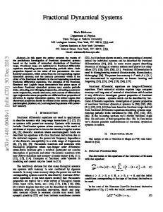
Existence of the resonance manifold in the presence of (scaled) detuning parameter ∆ = Eδ1a2 . The vertical axis represents ∆ 0 2 a1 and the horizontal axis λ = 3a . The domain II and the unbounded 2 domain I and III (both bounded by the parabola and the straight line) correspond with existence of the resonance manifold.

How is the effect of detuning in the case of existence of the resonance manifold? In the same way as before, in terms of parameters λ and ∆ = δ1 /(E0 a2 2 ), we can write for the existence of the resonant manifold (1.14)

0≤

−360λ+13−240∆ 3600λ2 −720λ−3

≤ 1.


29

In figure 2, the area marked by I, II and III represent the domains of existence of the resonance manifold in the parameter space. The parabolic boundary of the domain represents the first normal mode (q1 , p1 direction) and the straight line boundary the second normal mode. By fixing the detuning coefficient, we have a horizontal line on which we can move the resonance manifold from one normal mode to the other as we vary λ. The analysis can be repeated for fixed λ. The bold parts of the horizontal axes are the cases of exact resonance. Note that the intersection points are excluded as they correspond with the zero of the denominator in (1.13).

4.3. The degenerate case: γ2 = 4γ1 . Consider again the equations in (1.11). With the condition γ2 = 4γ1 , equations (1.11) become

ρ˙ 1 ρ˙ 2 χ˙

(1.15)

= 0 + O(ε3 ) = 0 + O(ε3 ) = ε2 (2γ1 E0 − 2δ1 ) + O(ε3 ).

System (1.15) immediately yields that at exact resonance there will be no resonance manifold. Another consequence is that there exist a critical energy Ec = γδ11 such that the last equation of (1.15) is zero, up to order ε3 . It means we have to include even higher order terms of the Hamiltonian in the analysis. From the normal form theory in section 2, we know that for the 1 : 2-resonance H5 does not contain resonant terms. Thus the next nonzero term would be derived from H6 . As a consequence, the equations for amplitudes and phases are all of the same order, i.e. O(ε4 ). It is also clear that in H6 besides terms which represent interaction between two degrees of freedom (resonant terms), there are also interactions between each degree of freedom with itself (terms of the form τ1 α τj β ). To avoid a lengthy calculation and as an example, we consider a problem where 3 a1 = a2 = 0. From the condition γ2 = 4γ1 we derive b2 = 3b1 + 16 b3 . Then the last equation of (1.15) becomes χ˙ = ε2

¡¡

− 34 b1 +

3 64 b3

¢

¡ ρ1 2 + 4 − 34 b1 +

3 64 b3

¢

¢ ρ2 2 − 2δ1 + O(ε3 ).

Introducing the critical energy Ec , we have a degeneration of the last equation which gives an additional relation, i.e. δ1 =

1 2

¡¡

− 34 b1 +

3 64 b3

¢

¡ ρ1 2 + 4 − 34 b1 +

3 64 b3

¢

¢ ρ2 2 .

We note also that for δ1 > 0 the critical energy exists providing b1
0 the critical energy only exist for κ < 16 1 and if δ < 0 for κ > 16 . 5. The elastic pendulum In this section we will study one of the classical mechanical examples with discrete symmetry. Consider a spring with spring constant s and length l◦ , a mass m is attached to the spring; g is the gravitational constant and l is the length of the spring under load in the vertical position. The spring can both oscillate in the vertical direction and swing like a pendulum. This is called the elastic pendulum. Let r(t) be the length of the spring at time t and ϕ the angular deflection of the spring from its vertical position. In [26] van der Burgh uses a Lagrangian formulation to analyze the elastic pendulum, while in this paper we will use a Hamiltonian formulation. The Hamiltonian is given by ³ ´ p2 1 (1.18) H = 2m p2r + rϕ2 + 2s (r − l◦ )2 − mgr cos ϕ, where pr = mr˙ and pϕ = mr2 ϕ. ˙

32


Introducing the elongation of the spring by z = r−l l , we translate the origin of the coordinate system to the fixed point of the system where the elastic pendulum is hanging vertically at rest. By dividing by l we normalize the length of the spring; we adjust also the momenta pz = lpr to keep the Hamiltonian structure. The Hamiltonian in the new variables is Ã ! µ ¶2 p2ϕ 1 sl2 l − l◦ 2 (1.19) H= pz + + z+ − mgl(z + 1) cos ϕ 2ml2 (z + 1)2 2 l √ Put α1 = ωz σ and α2 = ωϕ σ where σ = ml2 . We transform z = α1 z and ϕ = √ α1 ϕ. To preserve the Hamiltonian structure we also transform pz = α1 pz and √ pϕ = α2 pϕ . Expanding this Hamiltonian the two leading terms of the Hamiltonian are, H0 = 21 s(l − l◦ )2 − mgl H1 = √ω1z σ (sl (l − l◦ ) − mgl) z. √

We define the coordinate such that the pendulum is at rest in (pz , z, pϕ , ϕ) = (0, 0, 0, 0). As a consequence the linear term of the Hamiltonian is zero. Thus we have s(l − l◦ ) = mg. This condition restricts the ratio of the frequencies of the two oscillators, i.e. ωz /ωϕ > 1. The restriction is natural since at the equilibrium position the p resultant force of p gravitational force (mg) and spring force (s(l − l◦ )) is zero. With s/m = ωz and g/l = ωϕ , the remaining terms in the expansion of the Hamiltonian are ¡ ¢ ¡ ¢ H2 = 12 ωz z¡2 + p2z + 12 ω¢ϕ ϕ2 + p2ϕ ωϕ 1 zϕ2 − zp2ϕ H3 = √σω ³z 2 ´ ω 1 4 H4 = σ1 32 ωϕz z 2 p2ϕ − 24 ϕ ³ ´ ω 1 (1.20) H5 = − σ√1σωz 24 zϕ4 + 2 ωϕz z 3 p2ϕ µ ¶ ³ ´2 1 1 5 ωϕ 6 4 2 H6 = σ2 ωϕ 720 ϕ + 2 ωz z pϕ .. . As expected, the - relatively few - terms in the Hamiltonian are symmetric in the second degree of freedom and also in pz . Due to the restriction of the frequency ratio above, we will not have the 1 : λ-resonances with λ > 1. On the other hand, the symmetry condition on the second degree of freedom eliminates the 3 : 1-resonance as a lower order resonance. The next resonant term of this resonance arises from H8 . Thus, for lower order resonances, the remaining cases are the 2 : 1- and, if we allow small detuning, the 1 : 1-resonance. The 2 : 1-resonance has been intensively studied, see [26] or [16] for references. This resonance is the one with resonant terms of the lowest degree. As noted in [26], for the 1 : 1-resonance, second order averaging still gives only zero for both the amplitudes and the phases (this is not rendered correctly in [29]). It follows that the 1 : 1-resonance is also eliminated as a lower order resonance. The reason for this degeneracy is simple; by defining x = r sin(ϕ) and y = r cos(ϕ) we

5 The elastic pendulum

33

can transform (1.18) to 1 s m(x˙ 2 + y˙ 2 ) + (x2 + y 2 ) − mgy. 2 2 This means that for the 1 : 1-resonance we have the harmonic oscillator in which all solutions are periodic with the same period. Thus we have isochronism. Let us now assume that ωz /ωϕ 6= 1. Introduce the transformation z = r1 cos(ωz t + φ1 ), pz = −r1 sin(ωz t + φ1 ), ϕ = r2 cos(ωϕ t + φ2 ), and pϕ = −r2 sin(ωϕ t + φ2 ). Assuming ωz 6= 2ωϕ and rescaling with ε as usual we find the second-order averaged equations for amplitudes and phases H=

= 0 + O(²3 ) = 0 + O(²3 ) 3 (ωϕ − ωz )(ωz 2 + ωz ωϕ − 3ωϕ 2 ) 2 ρ1 + ψ˙ = −²2 (1.21) 4 (ωz + 2ωϕ )(2ωϕ − ωz )σ 3 2 1 (ωϕ − ωz )(ωz + 13ωz ωϕ + 20ωz ωϕ 2 − 28ωϕ 3 ) 2 ρ2 + O(²3 ), 16 ωz (ωz + 2ωϕ )(2ωz − ωϕ ) where ψ = ωϕ ψ1 − ωz ψ2 , ρ1 and ρ2 are the approximations of r1 and r2 , ψ1 and ψ2 are the approximations of φ1 and φ2 , respectively. The resonance manifold is determined by the requirement that the right hand side of equation (1.21) vanishes. √ This implies the resonance manifold exists for all resonances with ωz /ωϕ > ( 13 − 1)/2 ≈ 1.30277. . . (we exclude the 2 : 1-resonance and small detuning of it). We will now consider the most prominent higher order resonances which are possible for the elastic pendulum problem. We start with the 3 : 2- and the 4 : 1resonance. For both resonances we know that in general the resonant terms arises from H5 which implies that the amplitude variation will be zero up till second order averaging. This is in agreement with (1.21). To determine which resonance in the elastic pendulum arises from H5 , we have to normalize. ρ˙1 ρ˙2

ωz : ωϕ 4:1 4:3 6:1 3:1 8:1 3:2

Resonant Part dε H5 ε1/2 H7 ε3/2 H7 ε3/2 H8 ε2 H9 ε5/2 H10 ε3

Interaction time-scale ε−5/2 ε−7/2 ε−7/2 ε−4 ε−9/2 ε−5

Table 2. The table presents the most prominent higher order resonances of the elastic pendulum with lowest order resonant terms Hk . The third column gives the size of the resonance domain in which the resonance manifold is embedded while in the fourth column we find the time-scale of interaction in the resonance domain. The result is, for the 3 : 2-resonance, there is no resonant term in the normalized Hamiltonian up to degree 5. However, for the 4 : 1-resonance, there are resonant

34

Symmetry and Resonance in Hamiltonian Systems 2

1.5

1

0.5

0

−0.5

−1

−1.5

−2 −2.5

−2

−1.5

−1

−0.5

0

0.5

1

1.5

2

2.5

Figure 4.

The Poincaré map for the 6 : 1-resonance in the second degree of freedom (ε = 0.75 and the energy E = 5; large values for illustration purposes). The saddles are connected by heteroclinic cycles and inside the cycles (islands) are centers.

terms in the normalized Hamiltonian of degree 5. The conclusion is, after the firstorder 2 : 1-resonance, the 4 : 1-resonance is the most prominent resonance in the elastic pendulum. Following the analysis in section 3, we can also determine the sizes of the resonance manifolds which depend on the lowest degree of resonant terms in the normal form. We repeat this for cases in which the resonant terms arise in H7 , . . . , H10 . The results are summarized in table 2. Note that a low order resonance as the 3 : 1-resonance figures here at relatively high order. We checked our result numerically for some of the resonances by constructing the Poincaré map and by calculating the size of the resonance domain. In the numerical integrations we vary ε and study how this affects the size of the resonance manifold. We found confirmation for the 4 : 1-resonance and the 6 : 1-resonance, i.e. the numerical exponents are 0.4971 . . . and 1.4991 . . . respectively. As table 2 shows, the numerical integration takes a long time. Figure 4 shows the map for the 6 : 1-resonance. To avoid long computation times, we increased the value of ε. In figure 5 we demonstrate the size and visibility of the resonance domain as ε increases for the 6 : 1-resonance. In figure 6 the 4 : 1-resonance and the 6 : 1-resonance are compared. 6. Conclusion and comments In nearly all real-life applications symmetries and hidden symmetries play an important part. We have mentioned a large number of examples. We have shown that (reflection) symmetry assumptions strongly affect some of the lower order and higher order resonances in two degrees of freedom Hamiltonian systems. In those cases, the symmetry assumption on one of the degrees of freedom implies a degeneration of

6 Conclusion and comments

35

1.5

1.5

1

1

0.5

0.5

0.5

1 1.5

1.5

0.5

1

1.5

1

0.5

0.5

1

1.5

Figure 5. The 6 : 1-resonance. Part of the map in the second degree of freedom direction for several values of ε, the energy E = 5. The topleft figure is for ε = 0.25, the top-right figure is for ε = 0.5 and the figure below is for ε = 0.75.

the normal form. This degeneration forces us to extend the normalization as the resonant terms appear at higher order as compared with the case without symmetry assumptions. The conclusion is then that some of the lower order resonances behave like higher order ones. This makes sense since we know that for instance the 1 : 2 resonance can be viewed as 2 : 4 resonance or 4 : 8 resonance etc. In the general, mathematically generic case, lower order resonance corresponds with strong interaction between the modes while higher order resonance corresponds with weak interaction, restricted to resonance domains. This happens for instance in a model for a Protein Cluster and in the theory of galactic orbits. For symmetric potential problems in 1 : 2 resonance, we have shown that at a certain critical value of the energy, localized in phase-space at some distance of equilibrium, the system behaves like a strong resonance while for other values of the energy it produces higher order resonance. We note that the presence of this critical energy involves the detuning parameter. This is an intriguing new phenomenon and more analysis is needed to see what part this critical energy may play in applications. In applying the analysis to the elastic pendulum we have found a numerical confirmation of our analytic estimates of the size of the resonance domain. Also we have found a new hierarchy in the resonances due to two reasons. First because of physical restrictions the m : n resonances with m < n are eliminated. Secondly the

36

Symmetry and Resonance in Hamiltonian Systems 0

1.5 −0.1

−0.2 1

−0.3

0.5 −0.4

−0.5 0

−0.6

−0.5 −0.7

0.5

1

1.5

2

2.5

1.1

1.15

1.2

1.25

1.3

1.35

Figure 6. Part of the map in the second degree of freedom direction for the 4 : 1-resonance (left) and the 6 : 1-resonance (right);ε = 0.1 and the energy E = 5. symmetry assumption. As is well-known the 2 : 1 resonance is the most prominent resonance, the next one turns out to be the 4 : 1 resonance. It turns out that the 1 : 1-resonance of the elastic pendulum is a rather trivial case.

Acknowledgments J. M. Tuwankotta thanks the Mathematisch Instituut, Universiteit Utrecht, the Netherlands and CICAT TUDelft, for financial support during the execution of the research; he also thanks Lennaert van Veen, Menno Verbeek, Luis M. Artiles, Bob Rink and Martijn van Manen for many comments and discussions. J.M. Tuwankotta thanks Santi Goenarso for every support during a difficult time.

Bibliography [1] Arnol’d, V.I., Mathematical Methods of Classical Mechanics, Springer-Verlag, New York etc., 1978. [2] Bayly, P.V., Virgin, L.N., An empirical study of the stability of periodic motion in the forced spring-pendulum, Proceeding of the Royal Society of London A 443, pp. 391-408, 1993. [3] Binney, J., Tremaine, S., Galactic Dynamics, Princeton University Press, Princeton, 1994. [4] Birkhoff, G.D., Dynamical Systems, reprinted by American Mathematical Society, 1972. [5] Broer, H. W., Hoveijn, I., Lunter, G. A., Vegter, G.,Resonances in a spring-pendulum: algorithms for equivariant singularity theory, Nonlinearity 11 , no. 6, pp. 1569-1605, 1998. [6] Cicogna, G. Gaeta,G., Symmetry and Perturbation Theory in Nonlinear Dynamics, Lecture Notes in Physics m 57, Springer-Verlag, 1999. [7] Gaeta,G., Poincar´ e renormalized forms , Ann. Inst. Henri Poincar´ e, vol. 70, no. 6, 1999, pp. 461-514. [8] Ford, J., Lunsford, G.H., On the Stability of Periodic Orbits for Nonlinear Oscillator Systems in Regions Exhibiting Stochastic Behavior, J. Math. Phys., vol 13, pp. 700-705, 1972. [9] Fujii, A.H., Inchiki, W. Nonlinear dynamics of the tethered sub satellite systems in the station keeping phase, Journal of Guidance and Control, no. 20, vol. 2, pp. 403-406, 1997. [10] Golubitsky, M., Stewart, I., Schaeffer, D.G., Singularities and Groups in Bifurcation Theory, vol. 2, Applied Math. Sciences 69, Springer-Verlag, 1988. [11] Golubitsky, M., Stewart, I., Generic Bifurcation of Hamiltonian Systems with Symmetry, Physica D, vol 24, pp. 391-404, 1987. [12] H´ enon, M., Heiles, C.,The Applicability of the Third Integral of Motion: Some Numerical Experiments, The Astronomical Journal, vol. 69, no. 1, 1964. [13] Hitzl, D.L., The swinging spring-families of periodic solutions and their stability I, Astronautics & Astrophysics 40, pp. 147-159, 1975. [14] Hitzl, D.L., The swinging spring-invariant curves formed by quasi-periodic solutions III, Astronautics & Astrophysics 41, pp. 187-198, 1975. [15] Kozlov, V.V., Symmetries, Topology, and Resonances in Hamiltonian Mechanics, Ergebnisse der Mathematik und ihre Grenzgebiete 31, Springer-Verlag, 1996. [16] Nayfeh, A.H., Mook, D.T., Nonlinear Oscillations, Wiley-Interscience, New York, 1979. [17] Noid, D. W., Koszykowski, M. L., Marcus, R. A.,Semi classical calculation of bound states in multidimensional systems with Fermi resonance, J. Chem. Phys. 71, no. 7, pp. 2864-2873, 1971. [18] Numez-Yepez, H.N., Salas-Brito, A.L., Vargas, C.A., Onset of chaos in an extensible pendulum, Physics Letters A, no. 145, vol. 2/3, pp. 101-105, 1990. [19] Rigney, D.R., Goldberger, A.L., Nonlinear mechanics of the heart’s swinging during pericardial effusion, American Physiological Society, no. 257, pp. H1292-H1305, 1989. [20] Rupp, C.C., Laue, J.H., Shuttle/tethered satellite system, Journal of the Astronautical Sciences XXVI, vol. 1, pp. 1-17, 1978. [21] Sanders, J.A.,Are higher order resonances really interesting?, Celestial Mech. 16, pp. 421-440, 1978.

38

Bibliography

[22] Sanders, J.A., Verhulst, F., Approximations of Higher Order Resonances with an Application to Contopoulos’ Model Problem, in Asymptotic Analysis, from theory to application,(F.Verhulst, ed.), Lecture Notes Math. 711, pp. 209-228, Springer-Verlag, Heidelberg etc. (1979). [23] Sanders, J.A., Verhulst, F., Averaging Method on Nonlinear Dynamical System, Applied Math. Sciences 59, Springer-Verlag, New York etc., 1985. [24] Shidlovskaya, E.G., Schimansky-Geier L., Romanovsky, Yu. M., Nonlinear Vibrations in a 2Dimensional Protein Cluster Model with Linear Bonds, Zeitschrift f¨ ur Physikalische Chemie, Bd. 214, H. 1, S. 65-82, 2000. [25] van den Broek, B., Studies in Nonlinear Resonance, Applications of Averaging, Ph.D. Thesis University of Utrecht, 1988. [26] van der Burgh, A.H.P., On The Higher Order Asymptotic Approximations for the Solutions of the Equations of Motion of an Elastic Pendulum, Journal of Sound and Vibration 42, pp. 463-475, 1975. [27] Verhulst, F., Discrete Symmetric Dynamical Systems at the Main Resonances with Applications to Axi-symmetric Galaxies, Phil. Trans. Royal Society London 290 pp. 435-465, 1979. [28] Verhulst, F., Nonlinear Differential Equations and Dynamical Systems, 2nd ed., Springer Verlag, Berlin,1996. [29] Verhulst, F., Symmetry and Integrability in Hamiltonian Normal Forms, in Symmetry and Perturbation Theory, D. Bambusi and G. Gaeta (eds), Quaderni GNFM pp. 245-284, Firenze, 1998.

CHAPTER 2

Geometric Numerical Integration Applied to the Elastic Pendulum at Higher Order Resonance A joint work with G. R. W. Quispel Abstract. In this paper we study the performance of a symplectic numerical integrator based on the splitting method. This method is applied to a subtle problem i.e. higher order resonance of the elastic pendulum. In order to numerically study the phase space of the elastic pendulum at higher order resonance, a numerical integrator which preserves qualitative features after long integration times is needed. We show by means of an example that our symplectic method offers a relatively cheap and accurate numerical integrator.

Keywords. Hamiltonian mechanics, higher-order resonance, elastic pendulum, symplectic numerical integration, geometric integration. AMS classification. 34C15, 37M15, 65P10, 70H08

1. Introduction Higher order resonances are known to have a long time-scale behaviour. From an asymptotic point of view, a first order approximation (such as first order averaging) would not be able to clarify the interesting dynamics in such a system. Numerically, this means that the integration times needed to capture such behaviour are significantly increased. In this paper we present a reasonably cheap method to achieve a qualitatively good result even after long integration times. Geometric numerical integration methods for (ordinary) differential equations ([2, 10, 13]) have emerged in the last decade as alternatives to traditional methods (e.g. Runge-Kutta methods). Geometric methods are designed to preserve certain properties of a given ODE exactly (i.e. without truncation error). The use of geometric methods is particularly important for long integration times. Examples of geometric integration methods include symplectic integrators, volume-preserving integrators, symmetry-preserving integrators, integrators that preserve first integrals (e.g. energy), Lie-group integrators, etc. A survey is given in [10]. It is well known that resonances play an important role in determining the dynamics of a given system. In practice, higher order resonances occur more often than lower order ones, but their analysis is more complicated. In [12], Sanders was the first to give an upper bound on the size of the resonance domain (the region where interesting dynamics takes place) in two degrees of freedom Hamiltonian systems.

40

Geometric Numerical Integration ...

Numerical studies by van den Broek [16], however, provided evidence that the resonance domain is actually much smaller. In [15], Tuwankotta and Verhulst derived improved estimates for the size of the resonance domain, and provided numerical evidence that for the 4 : 1 and the 6 : 1 resonances of the elastic pendulum, their estimates are sharp. The numerical method they used in their analysis 1, however, was not powerful enough to be applied to higher order resonances. In this paper we construct a symplectic integration method, and use it to show numerically that the estimates of the size of the resonance domain in [15] are also sharp for the 4 : 3 and the 3 : 1 resonances. Another subtle problem regarding to this resonance manifold is the bifurcation of this manifold as the energy increases. To study this problem numerically one would need a numerical method which is reasonably cheap and accurate after a long integration times. In this paper we will use the elastic pendulum as an example. The elastic pendulum is a well known (classical) mechanical problem which has been studied by many authors. One of the reasons is that the elastic pendulum can serve as a model for many problems in different fields. See the references in [5, 15]. In itself, the elastic pendulum is a very rich dynamical system. For different resonances, it can serve as an example of a chaotic system, an auto-parametric excitation system ([17]), or even a linearizable system. The system also has (discrete) symmetries which turn out to cause degeneracy in the normal form. We will first give a brief introduction to the splitting method which is the main ingredient for the symplectic integrator in this paper. We will then collect the analytical results on the elastic pendulum that have been found by various authors. Mostly, in this paper we will be concerned with the higher order resonances in the system. All of this will be done in the next two sections of the paper. In the fourth section we will compare our symplectic integrator with the standard 4-th order Runge-Kutta method and also with an order 7 − 8 Runge-Kutta method. We end the fourth section by calculating the size of the resonance domain of the elastic pendulum at higher order resonance. 2. Symplectic Integration Consider a symplectic space Ω = R2n , n ∈ N where each element ξ in Ω has coordinate (q, p) and the symplectic form is dq ∧ dp. For any two functions F, G ∈ C ∞ (Ω) define ¶ n µ X ∂F ∂G ∂G ∂F {F, G} = − ∈ C ∞ (Ω), ∂q ∂p ∂q ∂p j j j j 1 which is called the Poisson bracket of F and G. Every function H ∈ C ∞ (Ω) generates a (Hamiltonian) vector field defined by {qi , H}, {pi , H}, i = 1, . . . , n. The dynamics of H is then governed by the equations of motion of the form q˙i ={qi , H} p˙i ={pi , H}, 1A Runge-Kutta method of order 7 − 8

i = 1, . . . , n.

2 Symplectic Integration

41

Let X and Y be two Hamiltonian vector fields, defined in Ω, associated with Hamiltonians HX and HY in C ∞ (Ω) respectively. Consider another vector field [X, Y ] which is just the commutator of the vector fields X and Y . Then [X, Y ] is also a Hamiltonian vector field with Hamiltonian H[X,Y ] = {HX , HY }. See for example [1, 7, 11] for details. We can write the flow of the Hamiltonian vector fields X as ϕX ;t = exp(tX) ≡ I + tX +

1 2 2! (tX)

+

1 3 3! (tX)

+ ···

(and so does the flow of Y ). By the Baker-Campbell-Hausdorff formula (see for example [13]), which yields a power series expansion for Z = Z(X, Y ) in terms of X and Y if exp(Z) = exp(X)exp(Y ), there exists a (formal) Hamiltonian vector field Z such that (2.1)

Z = (X + Y ) + 2t [X, Y ] +

t2 12

([X, X, Y ] + [Y, Y, X]) + O(t3 )

and exp(tZ) = exp(tX)exp(tY ), where [X, X, Y ] = [X, [X, Y ]] , and so on. Moreover, Yoshida (in [19]) shows that exp(tX)exp(tY )exp(tX) = exp(tZ), where (2.2)

Z = (2X + Y ) +

t2 6

([Y, Y, X] − [X, X, Y ]) + O(t4 ).

We note that in terms of the flow, the multiplication of the exponentials above means composition of the corresponding flow, i.e. ϕY ;t ◦ ϕX ;t . Let τ ∈ R be a small positive number and consider a Hamiltonian system with Hamiltonian H(ξ) = HX (ξ) + HY (ξ), where ξ ∈ Ω, and ξ˙ = X + Y . Using (2.1) we have that ϕY ;τ ◦ ϕX ;τ is (approximately) the flow of a Hamiltonian system ξ˙ = (X + Y ) + τ2 [X, Y ] + with Hamiltonian Hτ =HX + HY + +

2

τ 12

τ 2

τ2 12

([X, X, Y ] + [Y, Y, X]) + O(τ 3 ),

{HX , HY }

({HX , HX , HY } + {HY , HY , HX }) + O(τ 3 ).

Note that {H, K, F } = {H, {K, F }}. This mean that H − Hτ = O(τ ) or, in other words (2.3)

ϕY ;τ ◦ ϕX ;τ = ϕX+Y (τ ) + O(τ 2 ).

As before and using (2.2), we conclude that (2.4)

ϕX ; τ2 ◦ ϕY ;τ ◦ ϕX ; τ2 = ϕX+Y (τ ) + O(τ 3 ).

Suppose that ψX ;τ and ψY ;τ are numerical integrators of system ξ˙ = X and ˙ξ = Y (respectively). We can use symmetric composition (see [8]) to improve the accuracy of ψX+Y ;τ . If ψY ;τ and ψX ;τ are symplectic, then the composition forms a symplectic numerical integrator for X + Y . See [13] for more discussion; also [10] for references. If we can split H into two (or more) parts which Poisson commute with each other (i.e. the Poisson brackets between each pair vanish), then we have H = Hτ . This implies that in this case the accuracy of the approximation depends only on the accuracy of the integrators for X and Y . An example of this case is when we are integrating the Birkhoff normal form of a Hamiltonian system.

42

Geometric Numerical Integration ... 3. The Elastic Pendulum

Consider a spring with spring constant s and length l◦ to which a mass m is attached. Let g be the gravitational constant and l the length of the spring under load in the vertical position, and let r be the distance between the mass m and the suspension point. The spring can both oscillate in the radial direction and swing like a pendulum. This is called the elastic pendulum. See Figure (1) for illustration and [15] (or [18]) for references.

Figure 1. The elastic pendulum. where z = The phase space is R4 with canonical coordinate ξ = (z, ϕ, pz , pϕ ), p (r − l◦p )/l◦ . Writing the linear frequencies of the Hamiltonian as ωz = s/m and ωϕ = g/l, the Hamiltonian of the elastic pendulum becomes µ ³ ´ ³ ´2 ¶2 p2ϕ ωϕ 1 σ 2 (2.5) H = 2σ p2z + (z+1) + ω z + − σωϕ 2 (z + 1) cos ϕ, 2 2 z ωz where σ = ml2 . By choosing the right physical dimensions, we can scale out σ. We remark that for the elastic pendulum as illustrated in Figure 1, we have ωz ≤ ωϕ . See [15] for details. It is clear that this system possesses symmetry (2.6)

T : (z, ϕ, pz , pϕ , t) 7→ (z, −ϕ, pz , −pϕ , t)

and the reversing symmetries (2.7)

R1 : (z, ϕ, pz , pϕ , t) 7→ (z, ϕ, −pz , −pϕ , −t), R2 : (z, ϕ, pz , pϕ , t) 7→ (z, −ϕ, −pz , pϕ , −t).

If there exist two integers k1 and k2 such that k1 ωz + k2 ωϕ = 0, then we say ωz and ωϕ are in resonance. Assuming (|k1 |, |k2 |) = 1, we can divide the resonances in two types, e.g. lower order resonance if |k1 | + |k2 | < 5 and higher order resonance if |k1 | + |k2 | ≥ 5. In the theory of normal forms, the type of normal form of the Hamiltonian is highly dependent on the type of resonance in the system. See [1].

3 The Elastic Pendulum

43

In general, the elastic pendulum has at least one fixed point which is the origin of phase space. This fixed point is elliptic. For some of the resonances, there is also another fixed point which is of the saddle type, i.e. (z, ϕ, pz , pϕ ) = (−2(ωϕ /ωz )2 , π, 0, 0). From √ the definition of z, it is clear that the latter fixed point only exists for ωz /ωϕ > 2. The elastic pendulum also has a special periodic solution in which ϕ = pϕ = 0 (the normal mode). This normal mode is an exact solution of the system derived from (2.5). We note that there is no nontrivial solution of the form (0, ϕ(t), 0, pϕ (t)). Now we turn our attention to the neighborhood of the origin. We refer to [15] for the complete derivation of the following Taylor expansion of the Hamiltonian (we have dropped the bar) (2.8) with

H = H2 + εH3 + ε2 H4 + ε3 H5 + · · · , ¡ ¢ ¡ ¢ H2 = 12 ωz z 2 + p2z + 12 ωϕ ϕ2 + p2ϕ ¡ ¢ ω H3 = √ωϕz 12 zϕ2 − zp2ϕ ³ ´ ω 1 4 H4 = 32 ωϕz z 2 p2ϕ − 24 ϕ ³ ´ ω 1 H5 = − √1ωz 24 zϕ4 + 2 ωϕz z 3 p2ϕ .. .

In [17] the 2 : 1-resonance of the elastic pendulum has been studied intensively. At this specific resonance, the system exhibits an interesting phenomenon called auto-parametric excitation, e.g. if we start at any initial condition arbitrarily close to the normal mode, then we will see energy interchanging between the oscillating and swinging motion. In [3], the author shows that the normal mode solution (which is the vertical oscillation) is unstable and therefore, gives an explanation of the autoparametric behavior. Next we consider two limiting cases of the resonances, i.e. when ωz /ωϕ → ∞ and ωz /ωϕ → 1. The first limiting case can be interpreted as a case with a very large spring constant so that the vertical oscillation can be neglected. The spring pendulum then becomes an ordinary pendulum; thus the system is integrable. The other limiting case is interpreted as the case where l◦ = 0 (or very weak spring) 2. Using the transformation r = l(z + 1), x = r cos ϕ and y = r sin ϕ, we transform the Hamiltonian (2.5) to the Hamiltonian of the harmonic oscillator. Thus this case is also integrable. Furthermore, in this case all solutions are periodic with the same period which is known as isochronism. This means that we can remove the dependence of the period of oscillation of the mathematical pendulum on the amplitude, using this specific spring. We note that this isochronism is not derived from the normal form (as in [18]) but exact. 2This case is unrealistic for the model illustrated in Figure 1. A more realistic mechanical model with the same Hamiltonian (2.5) can be constructed by only allowing some part of the spring to swing

44


All other resonances are higher order resonances. In two degrees of freedom (which is the case we consider), for fixed small energy the phase space of the system near the origin looks like the phase space of decoupled harmonic oscillator. A consequence of this fact is that in the neighborhood of the origin, there is no interaction between the two degrees of freedom. The normal mode (if it exists), then becomes elliptic (thus stable). Another possible feature of this type of resonance is the existence of a resonance manifold containing periodic solutions (see [4] paragraph 4.8). We remark that the existence of this resonance manifold does not depend on whether the system is integrable or not. In the resonance domain (i.e. the neighborhood of the resonant manifold), interesting dynamics (in the sense of energy interchanging between the two degrees of freedom) takes place (see [12]). Both the size of the domain where the dynamics takes place and the time-scale of interaction are characterized by ε and the order of the resonance, i.e. the estimate of the size of the domain is ³ m+n−4 ´ dε = O ε 2 m+n

and the time-scale of interactions is O(ε− 2 ) for ωz : ωϕ = m : n with (m, n) = 1. 3 We note that for some of the higher order resonances where ωz /ωϕ ≈ 1 the resonance manifold fails to exist. See [15] for details. 4. Numerical Studies on the Elastic Pendulum One of the aims of this study is to construct a numerical Poincaré map (P) for the elastic pendulum in higher order resonance. As is explained in the previous section, interesting dynamics of the higher order resonances takes place in a rather small part of phase space. Moreover, the interaction time-scale is also rather long. For these two reasons, we need a numerical method which preserves qualitative behavior after a long time of integration. Obviously by decreasing the time step of any standard integrator (e.g. Runge-Kutta method), we would get a better result. As a consequence however, the actual computation time would become prohibitively long. Under these constraints, we would like to propose by means of an example that symplectic integrators offer reliable and reasonably cheap methods to obtain qualitatively good phase portraits. We have selected four of the most prominent higher order resonances in the elastic pendulum. For each of the chosen resonances, we derive its corresponding equations of motion from (2.8). This is done because the dependence on the small parameter ε is more visible there than in (2.5). Also from the asymptotic analysis point of view, we know that (2.8) truncated to a sufficient degree has enough ingredients of the dynamics of (2.5). The map P is constructed as follows. We choose the initial values ξ◦ in such a way that they all lie in the approximate energy manifold H2 = E◦ ∈ R and in the section Σ = {ξ = (z, ϕ, pz , pϕ )|z = 0, pz > 0}. We follow the numerically constructed trajectory corresponding to ξ◦ and take the intersection of the trajectory 3Due to a particular symmetry, some of the lower order resonances become higher order

resonances ([15]). In those cases, (m, n) = 1 need not hold.

4 Numerical Studies on the Elastic Pendulum

45

with section Σ. The intersection point is defined as P(ξ◦ ). Starting from P(ξ◦ ) as an initial value, we go on integrating and in the same way we find P 2 (ξ◦ ), and so on. The best way of measuring the performance of a numerical integrator is by comparing with an exact solution. Due to the presence of the normal mode solution (as an exact solution), we can check the performance of the numerical integrator in this way (we will do this in section 4.2) . Nevertheless, we should remark that none of the nonlinear terms play a part in this normal mode solution. Recall that the normal mode is found in the invariant manifold {(z, ϕ, pz , pϕ |ϕ = pϕ = 0} and in this manifold the equations of motion of (2.8) are linear. Another way of measuring the performance of an integrator is to compare it with other methods. One of the best known methods for time integration are the RungeKutta methods (see [6]). We will compare our integrator with a higher order (7-8 order) Runge-Kutta method (RK78). The RK78 is based on the method of RungeKutta-Felbergh ([14]). The advantage of this method is that it provides step-size control. As is indicated by the name of the method, to choose the optimal step size it compares the discretizations using 7-th order and 8-th order Runge-Kutta methods. A nice discussion on lower order methods of this type, can be found in [14] pp. 448-454. The coefficients in this method are not uniquely determined. For RK78 that we used in this paper, the coefficients were calculated by C. Simo from the University of Barcelona. We will also compare the symplectic integrator (SI) to the standard 4-th order Runge-Kutta method. We will first describe the splitting of the Hamiltonian which is at the core of the symplectic integration method in this paper. By combining the flow of each part of the Hamiltonian, we construct a 4-th order symplectic integrator. The symplecticity is obvious since it is the composition of exact Hamiltonian flows. Next we will show the numerical comparison between the three integrators, RK78, SI and RK4. We compare them to an exact solution. We will also show the performance of the numerical integrators with respect to energy preservation. We note that SI are not designed to preserve energy (see [10]). Because RK78 is a higher order method (thus more accurate), we will also compare the orbit of RK4 and SI. We will end this section with results on the size of the resonance domain calculated by the SI method.

4.1. The Splitting of the Hamiltonian . Consider again the expanded Hamiltonian of the elastic pendulum (2.8). We split this Hamiltonian into integrable parts: H = H 1 + H 2 + H 3 , where

(2.9)

ωϕ 1 1 H 1 =ε √ zϕ2 − ε2 ϕ4 − ε3 √ zϕ4 + · · · 2 ωz 24 24 ωz ωϕ 3 ωϕ 2 2 2ωϕ H 2 = − ε √ zp2ϕ + ε2 z pϕ − ε3 √ z 3 p2ϕ + · · · ωz 2 ωz ωz ωz ¡ 2 ¢ 1 ¡ 2 ¢ 3 1 2 2 H = 2 ωz z + pz + 2 ωϕ ϕ + pϕ .

46


Note that the equations of motion derived from each part of the Hamiltonian can be integrated exactly; thus we know the exact flow ϕ1;τ , ϕ2:τ , and ϕ3;τ corresponding to H 1 ,H 2 , and H 3 respectively. This splitting has the following advantages. • It preserves the Hamiltonian structure of the system. • It preserves the symmetry (2.6) and reversing symmetries (2.7) of H. • H 1 and H 2 are of O(ε) compared with H (or H 3 ). Note that, for each resonance we will truncate (2.9) up to and including the degree where the resonant terms of the lowest order occur. We define (2.10)

ϕτ = ϕ1;τ /2 ◦ ϕ2;τ /2 ◦ ϕ3;τ ◦ ϕ2;τ /2 ◦ ϕ1;τ /2 .

From section 2 we know that this is a second order method. Next we define γ = √ 1/(2 − 3 2) and ψτ = ϕγτ ◦ ϕ(1−2γ)τ ◦ ϕγτ to get a fourth order method. This is known as the generalized Yoshida method (see [10]). By, Symplectic Integrator (SI) we will mean this fourth order method. This composition preserves the symplectic structure of the system, as well as the symmetry (2.6) and the reversing symmetries (2.7). This is in contrast with the Runge-Kutta methods which only preserves the symmetry (2.6), but not the symplectic structure, nor the reversing symmetries (2.7). As a consequence the Runge-Kutta methods do not preserve the KAM tori caused by symplecticity or reversibility. 4.2. Numerical Comparison between RK4, RK78 and SI . We start by comparing the three numerical methods, i.e. RK4, RK78, and SI. We choose the 4 : 1-resonance, which is the most prominent higher order resonance, as a test problem. We fix the value of the energy (H2 ) to p be 5 and take ε = 0.05. Starting at the initial condition z(0) = 0, ϕ(0) = 0, pz = 5/2, and p pϕ (0) = 0, wepknow that the exact solution we are approximating is given by ( 5/2 sin(4t), 0, 5/2 cos(4t), 0). We integrate the equations of motion up to t = 105 seconds and keep the result of the last 10 seconds to have time series z(tn ) and pz (tn ) produced by each integrator. Then we define a sequence sn = 99990 + 5n/100, n = 0, 1, . . . , 200. Using an interpolation method, for each of the time series we calculate the numerical z(sn ). In figure 2 we plot the error function z(sn ) − z(sn ) for each integrator. The plots in Figure in 2 clearly indicate the superiority of RK78 compared with the other methods (due to the higher order method). The error generated by RK78 is of order 10−7 for an integration time of 105 seconds. The minimum time step taken by RK78 is 0.0228 and the maximum is 0.0238. The error generated by SI on the other hand, is of order 10−5 . The CPU time of RK78 during this integration is 667.75 seconds. SI completes the computation after 446.72 seconds while RK4 only needs 149.83 seconds. We will now measure how well these integrators preserve energy. We start integrating from an initial condition z(0) = 0, ϕ(0) = 1.55, pϕ (0) = 0 and pz (0) is determined from H 3 = 5 (in other word we integrate on the energy manifold H = 5 + O(ε)). The small parameter is ε = 0.05 and we integrate for t = 105 seconds.


47

2 1 0 −1 −2 9.999 9.9991 −7 x 10 4

9.9992

9.9993

9.9994

9.9995

9.9996

9.9997

9.9998

9.9999

10 4

x 10

2 0 −2 −4 9.999 9.9991 −5 x 10 4

9.9992

9.9993

9.9994

9.9995

9.9996

9.9997

9.9998

9.9999

10 4

x 10

2 0 −2 −4 9.999

9.9991

9.9992

9.9993

9.9994

9.9995

9.9996

9.9997

9.9998

9.9999

10 4

x 10

Figure 2. Plots of the error function z(sn ) − z(sn ) against time. The upper figure is the result of RK4, the middle figure is RK78 and the lower figure is of SI. The time of integration is 105 with a time step for RK4 and SI of 0.025. 5.0005 5 5

4.9995 4.999

4.995

4.9985 4.99

4.998 9.999

9.9991

9.9992

9.9993

9.9994

9.9995

9.9996

9.9997

9.9998

9.9999

10 4

4.9975

x 10

1.637

4.997

1.636

4.9965

1.635

4.996

1.634

4.9955

1.633

9.9993

9.9993

9.9994

9.9994

9.9995

9.9995

9.9996

9.9997

9.9997

9.9998

9.9998 4

x 10

1.632 9.999

9.9991

9.9992

9.9993

9.9994

9.9995

9.9996

9.9997

9.9998

9.9999

10 4

x 10

Figure 3. Plots of the energy against time. The solid line represents the results from SI. The line with ’+’ represents the results from RK4 and the line with ’◦’ represents the results from RK78. On the left hand plot, we show the results of all three methods with the time step 0.01. The time step in the right hand plots is 0.05. The results from RK4 are plotted seperately since the energy has decreased significantly compared to the other two methods.

For RK78, the integration takes 667.42 second of CPU time. For RK4 and SI we used the same time step, that is 10−2 . RK4 takes 377.35 seconds while SI takes 807.01 seconds of CPU time. It is clear that SI, for this size of time step, is inefficient with regard to CPU time. This is due to the fact that to construct a higher order method we have to compose the flow several times. We plot the results of the last 10 seconds of the integrations in Figure 3. We note that in these 10 seconds, the largest time step used by RK78 is 0.02421. . . while the smallest is 0.02310. . . . It is

48


clear from this, that even though the CPU time of RK4 is very good, the result in the sense of conservation of energy is rather poor relative to the other methods. We increase the time step to 0.05 and integrate the equations of motion starting at the same initial condition and for the same time. The CPU time of SI is now 149.74 while for the RK4 it is 76.07. Again, in Figure 3 (the right hand plots) we plot the energy against time. A significant difference between RK4 and SI then appears in the energy plots. The results of symplectic integration are still good compared with the higher order method RK78. On the other hand, the results from RK4 are far below the other two. 4.3. Computation of the Size of the Resonance Domain. Finally, we calculate the resonance domain for some of the most prominent higher order resonances for the elastic pendulum. In Figure 4 we give an example of the resonance domain for the 4 : 1 resonance. We note that RK4 fails to produce the section. On the 1.8 1.7

1.7

1.6

1.6 1.5

1.5

1.4

1.4

1.3 1.3 1.2 1.2

1.1

1.1

1 0.4

0.5

0.6

0.7

0.8

0.9

0.4

2

2

1.5

1.5

1

1

0.5

0.5

0

0

−0.5

−0.5

−1

−1

−1.5

−1.5

−2 −2

−1

0

1

2

−2 −2

0.5

−1

0.6

0.7

0

0.8

0.9

1

1

2

Figure 4.

Resonance domain for the 4 : 1-resonance. The plots on the left are the results from SI while the right hand plots are the results from RK78. The vertical axis is the pϕ axis and the horizontal axis is ϕ. The time step is 0.05 and ε = 0.05. In the top figures, we blow up a part of the pictures underneath.

other hand, the results from SI are still accurate. We compare the results from SI and RK78 in Figure 4. After 5 × 103 seconds, one loop in the plot is completed. For that time of integration, RK78 takes 34.92 seconds of CPU time, while SI takes only 16.35 seconds. This is very useful since to calculate for smaller values of ε and higher resonance cases, the integration time is a lot longer which makes it impractical to use RK78.


49

In Table 1 we list the four most prominent higher order resonances for the elastic pendulum. This table is adopted from [15] where the authors list six of them. Resonance Resonant Analytic Numerical Error part logε (dε ) logε (dε ) 4:1 H5 1/2 0.5091568 0.01 6:1 H7 3/2 1.5079998 0.05 4:3 H7 3/2 1.4478968 0.09 3:1 H8 2 2.0898136 0.35 Table 1. Comparison between the analytic estimate and the numerical computation of the size of the resonance domain of four of the most prominent higher order resonances of the elastic pendulum. The second column of this table indicates the part of the expanded Hamiltonian in which the lowest order resonant terms are found.

−0.5

−1

−1.5

−2

−2.5

−3

−3.5

−4

−4.5

−5

−5.5 −3

−2.5

−2

−1.5

−1

−0.5

Figure 5. Plots of log(dε ) against log(ε) for various resonances. The 4 : 1-resonance is plotted using ’−◦’, the 3 : 1-resonance is using ’−+’, the 4 : 3-resonance is using ’−×’ and the 6 : 1 resonance is using ’−∗’.

The numerical size of the domain in table 1 is computed as follows. We first draw several orbits of the Poincaré maps P. Using a twist map argument, we can locate the resonance domain. By adjusting the initial condition manually, we then approximate the heteroclinic cycle of P. See figure 4 for illustration. Using interpolation we construct the function ro (θ) which represent the distance of a point in the outer cycle to the origin and θ is the angle with respect to the positive horizontal axis. We do the same for the inner cycle and then calculate maxθ |ro (θ) − ri (θ)|. The higher the resonance is, the more difficult to compute the size of the domain in this way. For resonances with very high order, manually approximating the heteroclinic cycles would become impractical, and one could do the following. First we have to

50


calculate the location of the fixed points of the iterated Poincaré maps numerically. Then we can construct approximations of the stable and unstable manifolds of one of the saddle points. By shooting to the next saddle point, we can make corrections to the approximate stable and unstable manifold of the fixed point. 5. Discussion In this section we summarize the previous sections. First the performance of the integrators is summarized in table 2.

CPU time The 4 : 1 Preservation of H resonance Orbital Quality Section Quality The 6 : 1 Orbital Quality resonance Section Quality The 4 : 3 Orbital Quality resonance Section Quality The 3 : 1 Orbital Quality resonance Section Quality

RK4 149.83 sec. Poor Poor — Poor — Poor — Poor —

Integrators RK78 SI 667.75 sec. 446.72 sec. Good Good Very good Good Good Good Good Good Good Good Good Good — Good Poor Good — Good

Table 2. Summary of the performance of the integrators. A bar — indicates that it is not feasible to obtain a surface of section for this resonance using this integrator. For the CPU time we have put ∆t ≈ 0.025 while integration time is t = 105 sec. The preservation of H is measured by checking the value of H after t = 105 sec.

As indicated in table 2, for the 4 : 3 and the 3 : 1 resonances, the higher order Runge-Kutta method fails to produce the section. This is caused by the dissipation term, artificially introduced by this numerical method, which after a long time of integration starts to be more significant. On the other hand, we conclude that the results of our symplectic integrator are reliable. This conclusion is also supported by the numerical calculations of the size of the resonance domain (listed in Table 2). In order to force the higher order Runge-Kutta method to be able to produce the section, one could also do the following. Keeping in mind that RK78 has automatic step size control based on the smoothness of the vector field, one could manually set the maximum time step for RK78 to be smaller than 0.02310. This would make the integration times extremely long however. We should remark that in this paper we have made a number of simplifications. One is that we have not used the original Hamiltonian. The truncated Taylor expansion of (2.5) is polynomial. Somehow this may have a smoothing effect on the Hamiltonian system. It would be interesting to see the effect of this simplification

5 Discussion

51

on the dynamics of the full system. Another simplification is that, instead of choosing our initial conditions in the energy manifold H = C, we are choosing them in H 3 = C. By using the full Hamiltonian instead of the truncated Taylor expansion of the Hamiltonian, it would become easy to choose the initial conditions in the original energy manifold. Nevertheless, since in this paper we always start in the section Σ, we know that we are actually approximating the original energy manifold up to order ε2 . We also have not used the presence of the small parameter ε in the system. As noted in [9], it may be possible to improve our symplectic integrator using this small parameter. Still related to this small parameter, one also might ask whether it would be possible to go to even smaller values of ε. In this paper we took e−3 < ε < e−0.5 . As noted in the previous section, the method that we apply in this paper can not be used for computing the size of the resonance domain for very high order resonances. This is due to the fact that the resonance domain then becomes exceedingly small. This is more or less the same difficulty we might encounter if we decrease the value of ε. Another interesting possibility is to numerically follow the resonance manifold as the energy increases. As noted in the introduction, this is a numerically difficult problem. Since this symplectic integration method offers a cheap and accurate way of producing the resonance domain, it might be possible to numerically study the bifurcation of the resonance manifold as the energy increases. Again, we note that to do so we would have to use the full Hamiltonian.

Acknowledgements J.M. Tuwankotta thanks the School of Mathematical and Statistical Sciences, La Trobe University, Australia for their hospitality when he was visiting the university. Thanks to David McLaren of La Trobe University, and Ferdinand Verhulst, Menno Verbeek and Michiel Hochstenbach of Universiteit Utrecht, the Netherlands for their support and help during the execution of this research. Many thanks also to Santi Goenarso for every support she has given. We are grateful to the Nederlandse Organisatie voor Wetenschappelijk Onderzoek (NWO) and to the Australian Research Council (ARC) for financial support.

Bibliography [1] Arnol’d, V.I., Mathematical Methods of Classical Mechanics, Springer-Verlag, New York etc., 1978. [2] Budd, C.J., Iserles, A., eds. Geometric Integration, Phil. Trans. Roy. Soc. 357 A, pp. 943-1133, 1999. [3] Duistermaat, J.J., On Periodic Solutions near Equilibrium Points of Conservative Systems, Archive for Rational Mechanics and Analysis, vol. 45, num. 2, 1972. [4] Guckenheimer, J., Holmes, P., Nonlinear Oscillations, Dynamical Systems, and Bifurcations of Vector Fields, Springer-Verlag, New York etc., 1983. [5] Georgiou, I.,T., On the global geometric structure of the dynamics of the elastic pendulum, Nonlinear Dynamics 18,no. 1, pp. 51-68, 1999. [6] Hairer, E., Nørsett, S.P., Wanner, G., Solving Ordinary Differential Equations, SpringerVerlag, New York etc.,1993. [7] Marsden,J.E., Ratiu, T.S., Introduction to Mechanics and Symmetry,Text in Applied Math. 17, Springer-Verlag, New York etc., 1994. [8] McLachlan, R.I., On the Numerical Integration of Ordinary Differential Equations by Symmetric Composition Methods, SIAM J. Sci. Comput., vol. 16, no.1, pp. 151-168, 1995. [9] McLachlan, R.I., Composition Methods in the Presence of Small Parameters, BIT, no.35, pp. 258-268, 1995. [10] McLachlan, R.I., Quispel, G.R.W., Six Lectures on The Geometric Integration of ODEs, to appear in Foundations of Computational Mathematics, Oxford 1999, eds. R.A. De Vore et. al., Cambridge University Press. , Cambridge. [11] Olver, P.J., Applications of Lie Groups to Differential Equations, Springer-Verlag, New York etc. 1986. [12] Sanders, J.A.,Are higher order resonances really interesting?, Celestial Mech. 16, pp. 421-440, 1978. [13] Sanz-Serna, J.-M., Calvo, M.-P Numerical Hamiltonian Problems, Chapman Hall, 1994. [14] Stoer, J., Bulirsch, R.,Introduction to Numerical Analysis, 2nd ed., Text in Applied Math. 12, Springer-Verlag, 1993. [15] Tuwankotta, J.M., Verhulst, F., Symmetry and Resonance in Hamiltonian Systems, SIAM J. on Appl. Math., vol 61, no 4, pp. 1369-1385, 2000. [16] van den Broek, B., Studies in Nonlinear Resonance, Applications of Averaging, Ph.D. Thesis University of Utrecht, 1988. [17] van der Burgh, A.H.P., On The Asymptotic Solutions of the Differential Equations of the Elastic Pendulum, Journal de M´ ecanique, vol. 7. no. 4, pp. 507-520, 1968. [18] van der Burgh, A.H.P., On The Higher Order Asymptotic Approximations for the Solutions of the Equations of Motion of an Elastic Pendulum, Journal of Sound and Vibration 42, pp. 463-475, 1975. [19] Yoshida, H., Construction of Higher Order Symplectic Integrators, Phys. Lett. 150A, pp. 262268, 1990.

CHAPTER 3

Hamiltonian systems with Widely Separated Frequencies A joint work with Ferdinand Verhulst Abstract. In this paper we study two degree of freedom Hamiltonian systems and applications to nonlinear wave equations. Near the origin, we assume that near the linearized system has purely imaginary eigenvalues: ±iω1 and ±iω2 , with 0 < ω2 /ω1 ¿ 1 or ω2 /ω1 À 1, which is interpreted as a perturbation of a problem with double zero eigenvalues. Using the averaging method, we compute the normal form and show that the dynamics differs from the usual one for Hamiltonian systems at higher order resonances. Under certain conditions, the normal form is degenerate which forces us to normalize to higher degree. The asymptotic character of the normal form and the corresponding invariant tori is validated using KAM theorem. This analysis is then applied to widely separated mode-interaction in a family of nonlinear wave equations containing various degeneracies.

Keywords. Hamiltonian mechanics, resonance, normal forms, widely separated frequencies .

1. Introduction The dynamics of two degrees of freedom Hamiltonian systems near stable equilibrium is relatively well understood; see for instance [3] pp.258-270, [11] pp.212-226. Resonance is known to play an important role in the dynamics of a system of differential equations. The presence of resonance in a system significantly changes the behavior of the system. Consider for instance the flow on a torus with irrational slope − which corresponds to the non-resonant case − compared to the flow on a torus with rational slope. Orbits of the system in the first case are dense while in the second case, all solutions are periodic. In two degrees of freedom Hamiltonian systems, one can divide the resonances into three classes, namely first order resonances (also known as Fermi resonances), second order resonances, and higher order resonances (see [24] pp.146-162 for details). For systems in first order resonance, it is known that they may display parametric

56

Hamiltonian systems ...

excitation. This behavior is characterized by energy transfer between the degrees of freedom. This energy transfer is already apparent on a relatively short time-scale for almost all solutions (see [26]). However, the presence of a discrete symmetry may change the situation (see for instance [22, 27]). The higher order resonances also show some energy exchange but on a much smaller scale and on a much longer time-scale (see [23, 27]). In this paper, we consider two degrees of freedom Hamiltonian systems with widely separated frequencies: the ratio between the frequencies is either very small or very large. The small parameter ε is introduced into the system by rescaling the variables in the usual way. Such a system can be seen as a Hamiltonian system at an extreme high order resonance. One might expect that if the natural frequency ratio is 1 : ε, then the system behaves like a non-resonant two degrees of freedom Hamiltonian system. We show in this paper that this assumption produces somewhat different phenomena than expected. The phase-space of a non-resonant Hamiltonian system near the origin is foliated by invariant tori. These tori persist (by KAM theorem) under a Hamiltonian perturbation. In the case of widely separated frequencies, the phase space is nearly filled up with unbounded solutions, except for a very small domain near the elliptic equilibrium point. For ε = 0 the system is linear with double zero eigenvalues of the equilibrium at the origin. Broer et. al. in [5] (or in [6] for more explanation), studied this class of Hamiltonian systems in a more general setting. These systems can be divided into two cases, i.e. the semi-simple case and the non semi-simple case. Using normal form theory and singularity theory, the above authors give a bifurcation analysis near the equilibrium. The codimension of the equilibrium point is 1 for the non semi-simple case and 3 for the semi-simple case. Their paper also describes the universal unfolding of the equilibrium point. In our paper we consider only the semi-simple case. We extend the normal form analysis of [5] by considering a number of possible degeneracies arising in applications. We are also interested in describing the dynamics (in time) of the system which, in a sense, also supplements the analysis done in [5] or [6]. In applications, this type of problem arises quite naturally. For instance in the analysis of a model for atmospheric ultra-low frequency variability in [9], the author found a case where one of the natural frequencies in the system is as small as the nonlinear terms. However, there the system is not Hamiltonian. Nayfeh et. al. [19], [20] and Haller [12] treat comparable cases in mechanical engineering. For a recent result, see also Langford and Zhan in [16, 17]. We shall return to such problems in a separate paper. Lower order resonances produce more spectacular dynamics but higher order resonances appear more frequently in applications. For instance in wave equations, cases where the resonances are of the type that we consider in this paper are quite natural. This fact also motivated our study of this type of Hamiltonian system. In Section 2 we formulate our problem as one where perturbation theory and normal forms can be applied to approximate the full system. There are several ways

2 Mathematical formulation of the problem

57

to normalize a system of differential equations, namely using Lie-series, averaging, or using a generating function. For details on normalization using Lie-series, see [7, 8, 10], while for averaging or using a generating function see [2, 24]. We use the averaging method to compute the normal form. To verify the asymptotic nature of the normal form, the theory of averaging requires that we restrict ourselves to a domain of bounded solutions. For this, we approximate the locations of the saddle type equilibria of the system. The distance between these saddle points (if they exist) to the origin gives an indication of how large the domain of bounded solutions is. This is done in Section 3. We continue with the normal form computation to analyze the truncated normal form in Section 4 and 5. For some values of the parameters we have a degeneracy in the normal form, related to symmetry, which forces us to normalize to second-order. This situation is analyzed in Section 6 where we still find some nontrivial dynamics. We note that the assumption of the natural frequency being O(ε) affects the domain of bounded solutions. Keeping this in mind, we use KAM theory to show the validity of the normal form in Section 7. In Section 8 we discuss systems with widely separated frequencies which arise from the spectrum of evolution operators with initial-boundary conditions. Examples of such systems can be found in conservative nonlinear wave equations. It is shown that although there is no exchange of energy between the modes, there can be a strong phase interaction. 2. Mathematical formulation of the problem Consider a two degrees of freedom Hamiltonian (potential) system with Hamiltonian H = 21 (px 2 + x2 ) + 21 ε(py 2 + y 2 ) − ( 13 a1 x3 + a2 x2 y (3.1)

+ a3 xy 2 + 31 a4 y 3 ) − ( 41 b1 x4 + b2 x3 y + b3 x2 y 2 1 + b4 xy 3 + b5 y 4 ) + O(||(x, y, px , py )T ||5 ). 4

The Hamiltonian system is defined on R4 with coordinates (x, y, px , py ) and symplectic form dx ∧ dpx + dy ∧ dpy . We assume that ε is a small parameter: 0 < ε ¿ 1. We also assume that all of the constants aj , j = 1, . . . , 4 and bj , j = 1, . . . , 5 are O(1) with respect to ε. It is easy to see that for all ε > 0, the origin is an elliptic equilibrium. We re-scale the variables (and also time) using the small parameter to localize the system around the origin in the usual way (x = ε¯ x, . . .). The Hamiltonian (3.1) then becomes (we use the same notation for the rescaled variables and Hamiltonian) H = 21 (px 2 + x2 ) + 21 ε(py 2 + y 2 ) − ε( 13 a1 x3 + a2 x2 y + a3 xy 2 + 13 a4 y 3 ) − ε2 ( 14 b1 x4 + b2 x3 y + b3 x2 y 2 1 + b4 xy 3 + b5 y 4 ) + O(ε3 ). 4 Thus, we have a Hamiltonian perturbation of two harmonic oscillators with additional assumption that the basic frequency ratio in the system is 1 : ε. (3.2)

58


Remark 3.1. Two types of systems with widely separated frequencies. Consider a Hamiltonian systems with Hamiltonian ¡ ¢ ¡ ¢ (3.3) H = 21 ω1 p1 2 + q1 2 + 12 ω2 p2 2 + q2 2 + Hr . where Hr is a polynomial with degree at least three. There are two possibilities for the system generated by (3.3) to have widely separated frequencies. One might encounter the situation where ω2 = O(ε) as in the case of Hamiltonian (3.1). By rescaling the variables the Hamiltonian becomes ¡ ¢ ¡ ¢ (3.4) H = 21 p1 2 + q1 2 + 12 ε p2 2 + q2 2 + εH3 + ε2 H4 + . . . , where H3 represents the cubic terms, H4 the quartic. etc. We call this situation the first type of widely separated frequencies. The other possibility arises when ω1 = O(1/ε). By rescaling time (and also ε) we derive the Hamiltonian of the form H = 12 (p1 2 + q1 2 ) + 21 ε(p2 2 + q2 2 ) + εHr . In general, the Hamiltonian system derived from this Hamiltonian is still too complicated to analyze as all the nonlinear terms are of the same order. Thus, we localize around the origin by rescaling the variables. The asymptotic ordering in this case, however, is different from the one in (3.2) as the nonlinear terms become O(ε2 ): ¡ ¢ ¡ ¢ (3.5) H = 12 p1 2 + q1 2 + 12 ε p2 2 + q2 2 + ε2 H3 + ε3 H4 + . . . . We call this situation the second type.

In the unperturbed case, i.e. ε = 0, all solutions of the equations of motion derived from (3.2) are periodic with period 2π. Those solutions are of the form (x, y, px , py ) = (r◦ cos(t + ϕ◦ ), y◦ , −r◦ sin(t + ϕ◦ ), py◦ ), where r◦ , ϕ◦ , y◦ , and py◦ are determined by the given initial conditions. Moreover, all points of the form (0, y, 0, py ) ∈ R4 are critical corresponding with equilibria which is not a generic situation in Hamiltonian systems. We expect that most of these equilibria will be perturbed away when ε 6= 0. Consequently, most of the periodic solutions are also perturbed away. We use the averaging method to compute the normal form of the equations of motion derived from (3.2). Details on the averaging method can be found in [24]. The analysis is then valid up to order ε on the time-scale 1/ε at first-order, to order ε2 on the time-scale 1/ε at second-order. Before carrying out the normal form computation we first look at the domain where the solutions are bounded. 3. Domain of bounded solutions The theory of averaging requires the solutions of both the averaged and the original equations to stay in the interior of a bounded domain, at least for some time. In that domain, the averaging theorem guarantees the asymptotic character of the approximations. Thus, the existence of this domain is important.

4 Normal form computation

59

The equations of motion derived from (3.2) are

(3.6)

x˙ p˙x

= =

y˙ p˙y

= =

px −x + ε(a1 x2 + 2a2 xy + a3 y 2 ) +ε2 (b1 x3 + 3b2 x2 y + 2b3 xy 2 + b4 y 3 ) εpy ε(−y + a2 x2 + 2a3 xy + a4 y 2 ) +ε2 (b2 x3 + 2b3 x2 y + 3b4 xy 2 + b5 y 3 ).

We will approximate the equilibria of system (3.6). To do that, we set x = x◦ +εx1 + O(ε2 ) and y = y◦ + O(ε). It is clear that px = py = 0 at the equilibria. Substituting these into (3.6) we have two equilibria if a4 6= 0, i.e. (x, y, px , py ) = (0, 0, 0, 0) and (−εa3 /a4 2 , 1/a4 , 0, 0) while if a4 = 0 up to this approximation we have only one equilibrium, i.e. (0, 0, 0, 0). Define the potential function of the Hamiltonian (3.2), i.e. (3.7)

V (x, y) = 21 (x2 + εy 2 ) − ε( 31 a1 x3 + a2 x2 y + a3 xy 2 + 31 a4 y 3 ) − ε2 ( 41 b1 x4 + b2 x3 y + b3 x2 y 2 + b4 xy 3 + 41 b5 y 4 ) + O(ε3 ).

It is an easy exercise − by checking the second derivatives of (3.7) − to derive the stability of those equilibria found above. We conclude that (0, 0, 0, 0) is a center point and in the case where a4 6= 0 we have (−εa3 /a4 2 , 1/a4 , 0, 0) is a saddle point. The fact that we have a possibility of having a saddle point in an O(ε)-neighborhood of the center point implies the domain of bounded solutions to shrink in measure (at least as fast as ε as ε goes to zero). This is in contrast with the cases where all the natural frequencies are of the same order where the measure of the domain is independent of ε. 4. Normal form computation Consider again the equations of motion in (3.6). The equations for y and py in (3.6) are already in the Lagrange standard form. Thus we need only to transform the first two equations in (3.6). Putting x = r cos(t + ϕ) and px = −r sin(t + ϕ), the equations of motion (3.6) become ¡ © ϕ˙ = − 1r cos(t ª + ϕ) ε© a1 r2 cos2 (t + ϕ) + 2a2 r cos(t + ϕ)y 2 2 +a3 y 2 + ε2 b1 r3 cos3 (t + ϕ) ª¢+ 3b2 r cos (t + ϕ)y 2 3 +2b3 r cos(t + ϕ)y + b y 4 ¡ © r˙ = − sin(t +ªϕ) ε ©a1 r2 cos2 (t + ϕ) + 2a2 r cos(t + ϕ)y 2 2 +a3 y 2 + ε2 b1 r3 cos3 (t + ϕ) ª¢+ 3b2 r cos (t + ϕ)y (3.8) +2b3 r cos(t + ϕ)y 2 + b4 y 3 y˙ = εpy p˙y = ε(−y + a2 (r cos(t + ϕ))2 + 2a3 r cos(t + ϕ)y + a4 y 2 ) +ε2 (b2 (r cos(t + ϕ))3 + 2b3 (r cos(t + ϕ))2 y +3b4 r cos(t + ϕ)y 2 + b5 y 3 ). The right hand side of (3.8) is 2π-periodic in t. We note that the transformation to (ϕ, r) is not a symplectic transformation. However, the averaged equations of

60


motion are equivalent to the Birkhoff normal form of the equations of motion of (3.2). For some values of the parameters, first order averaging is not sufficient. For this reason we compute the normal form up to O(ε3 ) using second-order averaging. After applying the second-order averaging method to (3.2), we transform I = 21 r2 , ψ = t + ϕ. The averaged equations of motion then read ¡¡ ¢ ¢ ¢ ¡ ψ˙ = 1 − εa2 y − ε2 65 a1 2 + 34 b1 I + 12 a2 2 + a1 a3 + b3 y 2 I˙ = 0 (3.9) y˙ = εp¡y ¡ ¡ ¢ ¢ p˙y = ε −y¡ + a4 y 2 +¢a2 I¢ + ε2 2 12 a2 2 + a1 a3 + b3 yI + 2a3 2 + b5 y 3 , which is a Hamiltonian system with Hamiltonian H = I + εH1 + ε2 H2 ,

(3.10) where (3.11) and (3.12)

H2 = 12

¡

¢ y 2 + py 2 − a2 Iy − 31 a4 y 3

H1 =

1 2

¡5

¢ ¡ ¢ + 34 b1 I 2 + 12 a2 2 + a1 a3 + b3 y 2 I ¡ ¢ + 41 2a3 2 + b5 y 4 .

6 a1

2

This implies that the total energy H can be approximated by H = I + εH1 + ε2 H2 . As expected in such an extreme type of higher order resonance, the interaction between the two oscillators is weak in the sense that up to this approximation, there is no interchange of energy between the degrees of freedom. However, there is phase-interaction. In the next section we will first analyze the O(ε)-term of (3.9). Remark 3.2. As mentioned above, the transformation carrying (x, px ) into (r, ϕ) is not symplectic. Nevertheless, after averaging and transformation to coordinates (I, ψ) we re-gained the symplectic structure. The symplectic form is dψ ∧ dI + dy ∧ dpy . In the literature the pair (I, ψ) is known as symplectic polar coordinates. Remark 3.3. It is interesting to note that {H, I} = 0 where { , } is the Poisson bracket. The Hamiltonian (3.10) then can be viewed as a normalized H with respect to the S 1 -action defined by the flow of the unperturbed Hamiltonian, XI . Dividing out this action from the system (or equivalently fixing the value of I) leads to a reduced system (for reduction see [8]) which corresponds with a Poincaré section for the flow XH . This Poincaré section is an approximation of a section of the original flow XH . In contrast with the other cases in this family of Hamiltonian systems, − those in which the frequencies are of the same order − in this case the reduced space is R2 (for non flat reduced spaces, see for instance [7, 21]). Remark 3.4. In applications, symmetries arise naturally in a system. One can consider for instance the discrete symmetry φx : (x, y, px , py )T 7→ (−x, y, −px , py )T or φy : (x, y, px , py )T 7→ (x, −y, px , −py )T . If a Hamiltonian system is invariant

5 First order analysis of the averaged equations

61

under a symmetry φ then we have φ∗ H = H ◦ φ = H. The symmetry φx and φy is symplectic (they preserve the symplectic form). In [7] it is proved that the normalization can be done such that the symmetry φx or φy is preserved. For a y-symmetric Hamiltonian, i.e. a2 = a4 = b2 = b4 = 0, the normal form (3.9) is degenerate up to O(ε). However, a non-trivial dynamics is achieved as the second-order terms are included. On the other hands, for an x-symmetric Hamiltonian the normal form (3.9) is non-degenerate. 5. First order analysis of the averaged equations In this section we analyze the Hamiltonian system (3.9) up to order ε. What we mean is that we drop all terms of O(ε2 ), i.e.

(3.13)

ψ˙ I˙ y˙ p˙y

= = = =

1 − εa2 y 0 εp¡y ¢ ε −y + a4 y 2 + a2 I .

The solutions of system (3.13) approximate the solutions of system (3.8) to O(ε) on the time-scale 1/ε. The result of this section agree with [5, 6]. It is clear that I(t) ≥ 0 for all time and up to O(ε), it is related to the original Hamiltonian through H = I + εH1 . Instead of fixing the value of H we fix I = I◦ ∈ R. Thus, we are looking at the flow of Hamiltonian system (3.13), XH , restricted to the manifold I = I◦ . The reduced system (after rescaling time to τ = εt) is (3.14)

dy dτ dpy dτ

= =

py ¡ ¢ −y + a4 y 2 + a2 I◦ ,

which is a Hamiltonian system with Hamiltonian (3.11). In this reduced system, we might expect to have none, one or two equilibria. See also Remark 3.3. There are four (three independent) important parameters in the Hamiltonian system (3.14), namely a4 , a2 , I◦ , and (3.15)

D = 1 − 4a2 a4 I◦ .

As mentioned in the previous section, if a4 6= 0, in the ε-neighborhood of the origin we have another equilibrium of the saddle type. This equilibrium does not exist if a4 = 0. Furthermore, the reduced system (3.14) is degenerate if a4 = 0: it becomes a linear oscillator. Thus, for a4 = 0 we need to include quadratic terms in the normal form. We will do this in the next section. In this section we assume a4 6= 0. Let I◦ = 0, the flow XI◦ degenerates to a point. As a consequence, the flow XH in this case lives in a two-dimensional manifold defined by (0, 0) × R2 (or just R2 ). Furthermore, for I◦ = 0, we have D = 1 > 0. Thus, the dynamics in the manifold (0, 0) × R2 is the same as the dynamics of the reduced system for D > 0. Let us assume that I◦ > 0. The flow XI◦ defines a non-degenerate S 1 -action on the phase-space of system (3.13). Thus, the flow XH lives in S 1 ×R2 . If a2 6= 0, there are

62


y

Wu

py

D>0

Ws

D=0

D 0, there are two equilibria in the system (3.14): the √ saddle point (y s , 0) = ((1 + D)/(2a4 ), 0) and the center point (y c , 0) = ((1 − D)/(2a4 ), 0) (they correspond to H1 = hs and H1 = hc respectively). The center point (y c , 0) is surrounded by periodic orbits with period Z y◦+ 1 q (3.16) T =2 dy, − y◦ h − 12 y 2 + 21 a2 I◦ y + 13 a4 y 3 where y◦− and y◦+ are found by solving H1 = h for y if py = 0. If hs > hc then hc < h < hs . Orbits in which H1 > hs are unbounded 1. There exists a homoclinic connection: the component of H1 −1 (hs ) ∪ (y s , 0) which forms a closed curve. To translate this back to the full normalized system, we take the Cartesian product with the S 1 -action √ generated by XI◦ . At H1 = h√c , we have the stable periodic solution of the form ( 2I◦ cos((1 − εa2 y c )t + ϕ◦ ), y c , 2I◦ sin((1 − εa2 y c )t + ϕ◦ ), 0). The periodic solutions of (3.14) which are found if hc < h < hs , produce quasiperiodic solutions in the full normalized system. They live in two-dimensional tori 1 in R4 which are the bounded component of H1 −1 (h) Cartesian √ product with S s. At H1 = hs√ , we have the unstable periodic solution of the form ( 2I◦ cos((1 − εa2 y )t + ϕ◦ ), y s , 2I◦ sin((1 − εa2 y s )t + ϕ◦ ), 0). This periodic solution has two-dimensional unstable and stable manifolds which intersect transversally at the periodic orbit, and are also connected to each other to form a two-dimensional manifold in R4 homoclinic to the periodic solution. See Figure 2 for illustration. Let us consider the cases where D = 0 in equation (3.15) (we still assume a2 6= 0). There is only one equilibrium in the system (3.14), that is (1/2a4 , 0). The linearized 1We note that the converse does not hold since H −1 (h) might have two disconnected 1 components.

5 First order analysis of the averaged equations

63

Σ

y

y py

py

Figure 2.

An illustration for the geometry of the phase space of system (3.13) up to O(ε) in the case where D > 0 in (3.15). In this picture, the value of I is fixed. The thick lines represent the periodic orbits: the upper one is stable and the lower one is unstable. The unstable periodic solution is connected to itself by a 2-dimensional homoclinic manifold. In the two dimensional Poincaré section Σ, the dynamics is determined by (3.14).

system of (3.14) has double zero eigenvalues corresponding to a saddle-center bifurcation. As the center point and the saddle point of (3.14) coincide, the domain where the solutions are bounded vanishes. For D < 0, the situation is almost the same as the case where D = 0 except that there is no equilibrium in the system (3.14). For the full normalized system, the geometry of the phase-portrait for both D = 0 and D < 0 can be achieved by taking the cross product of the corresponding phase-portrait in Figure (1) with S 1 . Let a2 = 0. The system in (3.14) decouples up to O(ε) and the sign of D in the equation (3.15) is positive. We need only to note the existence of infinitely many periodic orbits of period T where T /2kπ ∈ N filling up a two dimensional torus (depending on the period) in phase-space. As we include the higher order terms in the normal form, these periodic solutions become quasi-periodic. The existence of the invariant manifold homoclinic to the periodic solution (S1 × H1 −1 (0)) is not affected by the fact that a2 = 0. Another degenerate case occurs when a4 = 0 (think of the y-symmetric Hamiltonian). In this case, the system (3.14) has one equilibrium for a fixed value of I◦ . The eigenvalues of this equilibrium are purely imaginary, i.e. ±i; all solutions of (3.14) are 2π-periodic. We shall discuss this in the next section.

64

Hamiltonian systems ... 6. Second order averaging if a4 = 0 Let a4 = 0. Then the Hamiltonians (3.11) and (3.12) reads ³ ´ 2 H1 = 12 (y − a2 I) + py 2 − 21 a2 I 2 ¡ ¢ ¡ ¢ ¡ ¢ H2 = 12 56 a1 2 + 34 b1 I 2 + 12 a2 2 + a1 a3 + b3 y 2 I + 41 2a3 2 + b5 y 4 ,

with corresponding equations of motion (after rescaling time) (3.17)

dy dτ py dτ

= =

py ¡ ¡ ¢ ¡ ¢ ¢ −y + a2 I + ε 2 12 a2 2 + a1 a3 + b3 yI + 2a3 2 + b5 y 3 ,

which is the reduced system for a fixed value of I. We first look for the equilibrium of (3.17). Consider the equation y 3 + γ1 y + γ2 = 0,

(3.18) where

−1 + ε(a2 2 + 2a1 a3 + 2b3 )I a2 I and γ2 = . 2 ε(2a3 + b5 ) ε(2a3 2 + b5 ) The discriminant of the equation (3.18) is γ1 =

(3.19)

D3 = (γ2 /2)2 + (γ1 /3)3 .

For (3.17) we have one, two or three equilibria. If D3 > 0, (3.18) has one real root. D3 = 0 gives two real roots while D3 < 0 corresponds to three real roots. We describe the phase-portrait of (3.17) in Figure 3. There are three different regions in the parameter space γ1 -γ2 corresponding to how many equilibria (3.17) has. Depending on the stability of each equilibrium, we have several possibilities for the phase-portraits. The stability of these equilibria can be derived as following. Let y◦ be a simple root of the equation (3.18) and write µ = 2a3 2 + b5 . If µ > 0, then (y◦ , 0) is a stable equilibrium. On the other hand if µ < 0, then (y◦ , 0) is a saddle point of the system (3.17). If y◦ is a double root, then (y◦ , 0) is an unstable equlibrium. Since the Hamiltonian of the system (3.17) is a quartic function, one can conclude that, if (3.17) has one or three equilibria, then all of them should correspond to simple roots of (3.18). If it has two equilibria, then one of them corresponds to a simple root while the other is a double root. From this analysis, we can derive the stability of each of the equilibria that exist in the system (3.17). We summarize this in Figure 3. Remark 3.5. In the case where µ = 2a3 2 + b5 = 0, the normalized system is again degenerate, in the sense that the dynamics is nothing but rotation around an elliptic equilibrium. We should then normalize to even higher degree. We expect to have more equilibria compared to those we found for the non-degenerate case. Apart from that, we expect no more complications. Remark 3.6. Notes on locations of the equilibria and their bifurcation One can see that both of γ1 and γ2 are O(1/ε). This implies that some of the equilibria found in this analysis might also be O(1/ε) and this analysis might not be applicable since it is far away from the domain where the normal form is a good

6 Second order averaging if a4 = 0

65

I γ2

II

III γ1

I

II

III y

py

µ0

Figure 3. Bifurcation diagram of the system (3.17). The curve depicted in this figure at the top is the curve (γ2 /2)2 + (γ1 /3)3 = 0. We draw the possible phase-portraits of the system (3.17) below this bifurcation diagram. For each region (indicated by the Roman numbers I, II, and III), we have two possibilities depending on the sign of µ = 2a3 2 + b5 . The dashed box indicates the location in the reduced space where the normal form is a good approximation of the full system. This situation is related with the one described as cusp catastrophe in [5, 6]. approximation of the system. In Figure 3 we place a dashed box around a particular equilibrium in the phase-portraits to indicate the domain where the normal form is a good approximation of the system. As stated in the last part of the previous section, in the case where a4 = 0 the first order analysis shows that the system has only one equilibrium. This equilibrium can be continued to a equilibrium in the system (3.17) (the one inside the box). During this continuation (by implicit function theorem) the stability of this equilibrium will not change.

66


Another way of looking at the bifurcation is the following. It is clear that γ1 6= 0 since aj and bj are independent of ε. This fact excludes the possibility of deforming the cubic equation (3.18) so that it has a single root with multiplicity three. Remark 3.7. It should be clear that these equilibria of the reduced system (if they survive), correspond to periodic orbits in the full system by taking the cross product of the equilibrium (y◦ , 0) with S 1 . The stability of these periodic orbits is the same as in the reduced system. Thus Figure 3 also serves as the bifurcation diagram for the periodic orbit in the full normalized system. 7. Application of the KAM theorem The celebrated Kolmogorov-Arnold-Moser (KAM) theorem is one of the most important theorems in perturbation theory of Hamiltonian dynamics. This theorem relates the dynamics from the normal form analysis to the dynamics in the full system, under some non-degeneracy condition. The theorem itself can be stated in a very general way (see [1] or [3]). As noted previously, the assumption on the frequencies implies that we can only guarantee the validity of the normal form in a rather small domain around the origin. However, the normal form of the system displays structurally stable behavior. Using the KAM theorem, we can validate this behavior. Consider a Hamiltonian system defined in a 2n-dimensional, symplectic space M in the action-angle variables (φ, J ) and symplectic form dφ∧dJ . The Hamiltonian of the system is H = H◦ (J )+εH1 (φ, J ). The unperturbed (ε = 0) Hamiltonian system is clearly integrable with integrals Ji , i = 1, . . . , n and the equations of motions are (3.20)

J˙ φ˙

= =

0 Λ(J ) = dH◦ (J ).

The phase space of the system (3.20) is foliated by invariant tori, parameterized by Jj = cj , j = 1, . . . , n. The KAM theorem concerns the preservation of these invariant tori as we turn on the (Hamiltonian) perturbation εH1 (φ, J ). The theorem guarantees the preservation of a large number of the invariant tori under the non-degeneracy condition that the symmetric n × n matrix dΛJ = d2 H◦ (J ) is invertible. In applying this fundamental theorem to a general Hamiltonian system with Hamiltonian H, one has to find an integrable Hamiltonian which is asymptotically close to H. For two degrees of freedom Hamiltonian systems, the truncated normal form is integrable. The asymptotic relation between the original and the truncated, normalized Hamiltonian system is also clear. Thus, it remains to see if the non-degeneracy condition is satisfied. For general two degrees of freedom Hamiltonian systems in higher order resonance (as well as the extreme type of higher order resonance), the non-degeneracy condition usually is not satisfied. The main difficulty is that the unperturbed integrable system is degenerate. The version of the KAM theorem stated below is applicable to higher order resonance cases. We will follow the discussion in [3].

8 Application to nonlinear wave equations

67

Consider the Hamiltonian system with Hamiltonian (3.21)

H = H00 (J1 ) + εH01 (J ) + ε2 H11 (φ, J ),

where J = (J1 , J2 ). This means that H00 is degenerate. The Hamiltonian (3.21) is called properly degenerate if ∂H00 ∂ 2 H01 6= 0 and 6= 0. ∂J1 ∂J2 2 The system H00 (J1 ) + εH01 (J ) is called the intermediate system. Theorem 3.8. In a properly degenerate system, a large subset of the phasespace of the system generated by Hamiltonian (3.21) is filled by invariant tori which are close to the invariant tori of the intermediate system: J is constant . The measure of the set of tori that dissapear √ under perturbation is exponentially small (O(exp(−constant/ε)) instead of O( ε) in the nondegenerate case). Remark 3.9. In a properly degenerate, two degrees of freedom Hamiltonian system, the situation is more regular in the sense that for all initial conditions, the values of the action variables remain forever near their initial values. See [3] for details and the reference therein. Applying Theorem 3.8 to our system, we define the intermediate system as H = I +εH1 , with H◦◦ = I. The action and angle variables for the one degree of freedom, Hamiltonian R y system generated by H1 can be calculated using the generating function S(J, y) = y◦ py dy. Thus we construct a symplectic transformation to bring (y, py ) to (J, φ) such that the equations of motion are of the form (3.20). The non-degeneracy condition on “the frequency” Λ(J) follows from the fact that the period function (3.16) in the case D > 0 in (3.15) and a4 6= 0, depends nonlinearly on hP . Thus, Theorem 3.8 is applicable to our system. 8. Application to nonlinear wave equations In this section we consider applications of the theory of widely spaced frequencies to nonlinear wave equations with initial-boundary values. Many studies have been devoted to such problems, see for instance the survey [28], also [4, 13, 14, 25]. In most of these studies the solution of the continuous system is expanded in an orthogonal series and then projected on a finite subspace using the Galerkin truncation method. This results in a finite set of ordinary differential equations. The next step is then to approximate the solution of this finite system by averaging, see for instance [14, 25], or multi-time scale methods, see [4]. Until now the applications have been to low-order resonance cases. 8.1. Formulation of the problem. Let Ω = [0, µπ] and L be a linear, selfadjoint, elliptic differential operator defined on a dense subset A ⊆ H◦ (Ω), i.e. L : A → H◦ (Ω), where H◦ (Ω) is a Hilbert space with an inner product h , i. It is

68


also assumed that L is essentially negative, i.e. its spectrum goes to −∞. Consider the initial-boundary value problem vtt − Lv v(0, t) v(x, 0) vt (x, 0)

(3.22)

= = = =

εf (v, vt , t) v(µπ, t) = 0 φ(x) ψ(x),

where µ ∈ R+ , 0 < ε ¿ 1, v = v(x, t) and f : D → H◦ (D ⊆ H1 × H◦ , for a Sobolev space H1 ). Important examples to take for L are ∂2 , the perturbed wave equation ∂x2 ∂2 − I, the perturbed dispersive wave equation L2 = ∂x2 ∂4 L3 = − 4 − p2 I, the perturbed beam equation, ∂x with I the identity operator and p ∈ N. In this paper we will be mainly concerned with the cases L = L1 or L = L2 . L1 =

The question of the existence and uniqueness of solutions of problem (3.22) can be settled in a standard way; see for instance for L = L1 and f (u, ut , t) = u3 in [14, 25]. In [25], the authors also consider the case where L = L2 . For L = L3 and f (u, ut , t) = u2 , the same question is studied in [4]. After applying the Galerkin truncation method an asymptotic solution of (3.22) is constructed. Let λn = −ωn 2 and Vn (x), n = 1, 2, · · · be the eigenvalues and the corresponding eigenfunctions of L. One of the implications of the assumptions on L is that the set of eigenfunctions {Vn , n = 1.2. · · · } form Pa denumerable, complete set in A. Thus, we can write for the solution v(x, t) = j aj (t)Vj (x). We substitute v(x, t) into (3.22) to obtain Ã∞ ! ∞ ∞ X X X ¡ ¢ a ¨j + ωj 2 aj Vj = f a j Vj , a˙ j Vj , t = f¯(x, t). 1

1

1

Projecting the last equation to the eigenspace generated by Vm , m = 1, · · · , N produces for m = 1, · · · , N (3.23)

a ¨m (t) + ωm 2 am (t) = hVm , f i(t),

∀t.

In [13, 25] it was realized that, choosing the initial condition φ and ψ to be effective only in some of the N modes, does not excite the other modes dramatically on a long time-scale. Thus, the eigenspace acts as an almost-invariant manifold. This observation was analyzed in [15], pp. 23-24, see also [14], where the author studies and proves the asymptotics of the manifold. In this section we will not discuss the approximation character of the truncation and averaging procedure of wave equations. This can be done, see [28], but it needs


69

a more detailed analysis which falls outside the scope of the present investigation. Our purpose in this section is to project (3.22) on a finite-dimensional space spanned by the eigenfunctions V1 and VM of the operator L corresponding to two widely separated eigenvalues (or modes). The projected system generated by V1 and VM (for M ∈ N) is (3.24)

a ¨1 + ω1 2 a1 a ¨M + ωM 2 aM

= =

εf¯1 εf¯M .

We have to choose M such that ω1 /ωM ¿ 1. 8.2. Scaling procedures. We can think of three different scalings applicable to problem (3.22): spatial domain scaling, time scaling, and scaling by localization. Spatial domain scaling is effected by putting x ¯ = x/µ and writing v(x, t) as u(¯ x, t). ¯ = [0, π]. Obviously, we This scaling transforms the spatial domain Ω = [0, µπ] to Ω also have to re-scale the linear operator L, the nonlinear function f , and the initial conditions φ and ψ. The nonlinear function f , and the initial conditions φ and ψ ˜ In general they will are transformed as v(x, t): by writing new functions f˜, φ˜ and ψ. depend on the parameter µ. With respect to the operator, spatial domain scaling results in scaling the eigenvalues of the operator. The first and second rescaled ˜ 1 = L1 /µ2 and L ˜ 2 = L1 /µ2 − I. Thus, the transformed initialoperators are L boundary value problem becomes (we have dropped the bar)

(3.25)

˜ utt − Lu = u(0, t) = u(x, 0) = ut (x, 0) =

εf˜(u, ut , t) u(π, t) = 0 ˜ φ(x) ˜ ψ(x),

˜ is L ˜ 1 or L˜2 . where L The time scaling procedure is done by putting τ = δ1 (ε)t where δ1 is an order function. Time scaling is usually carried out simultaneously with localization scaling: v¯ = δ2 (ε)v where δ2 is also an order function. It is easy to see that the scaling in v amounts to scaling in the amplitude a and its time derivative. Our goal is to use these scaling procedures to get widely separated frequencies in system (3.24) with main interest in L = L1 or L = L2 . Consider the situation where µ À 1, a large domain. Let M ∈ N be sufficiently large such that M/µ = O(1), compared to 1/µ = δ(ε) ¿ 1 (the order function δ(ε) is to be determined later). Before projecting to a finite-dimensional space by Galerkin truncation, we apply the spatial domain scaling which then brings us to (3.25). For the non-dispersive wave equation we have ω1 = O(δ(ε)) while ωM = O(1), which means we have a system with widely separated frequencies. Since this does not involve the time rescaling, we have the first type of widely separated frequencies. For the dispersive wave equation this approach does not produce a system with widely separated frequencies since ω1 = (1 + 1/µ) and ωM = (1 + M/µ) are both O(1).

70


If µ = 1, spatial domain scaling makes no sense. Again we choose M À 1, which implies ωM /ω1 À 1. This case is called the second type of widely separated frequencies in remark 3.1. By rescaling time, τ = ωM t, the projected equations of motion become ε ¯ a ¨1 + ( ωωM1 )2 a1 = ωM 2 f1 (3.26) ε ¯ a ¨M + aM = ωM 2 fM , in both the dispersive and non-dispersive case. This similarity is interesting. However, one can see that the nonlinearity in (3.26) is very small (of order O(ε/ωM 2 ). The dynamics in this case, if (3.26) is a Hamiltonian system, would be the same as the usual higher order resonance describe in [23, 27]. 8.3. The Hamiltonian equation utt − Lu = εf (u). We shall now consider perturbations such that the wave equation can be put in a Hamiltonian framework. Note that starting with a Hamiltonian wave equation, it is not obvious that Galerkin truncation again leads to a Hamiltonian system. Considering R4 as a symplectic space with symplectic form da1 ∧ db1 + daM ∧ dbM , we suppose that the right-hand side of system (3.24) is such that ∂Hr ∂Hr f¯1 = − and f¯2 = − , ∂a1 ∂aM for a function Hr (sufficiently smooth). Thus, system (3.24) has Hamiltonian H ¡ ¢ ¡ ¢ H = 21 a1 2 + ω1 2 b1 2 + 12 aM 2 + ω2 2 bM 2 + εHr , (we may have to re-scale ε). This Hamiltonian is not in the standard form (3.3). To bring it to the standard form, define a linear symplectic transformation √ √ √ √ T T (3.27) F : (a1 , aM , b1 , bM ) 7−→ (a1 / ω1 , aM / ω2 , ω1 b1 , ω2 bM ) . This transformation is also known as diagonalization in a Hamiltonian system. For ˜ r which depends on potential problems, the transformation F transform Hr to H ω1 or ω2 . This may become a problem with widely separated frequencies. The co˜ r also depend on the small parameter which changes the asymptotic efficients in H ordering of the nonlinear terms. In this subsection we will consider the typical perturbation f (u) = u3 which corresponds with a potential problem in the classical sense. It will become clear later that the transformation F simplifies the dynamics. First consider (3.25) with: L = L1 , µ À 1, ω1 = 1/µ and ωM = 1. After some computations one obtains that f (u) = u3 corresponds to the system (3.24) with the right-hand side functions (3.28) f˜1 = 3 a1 3 + 3a1 aM 2 and f˜2 = 3 aM 3 + 3a1 2 aM . 2

2

Transforming by F the Hamiltonian becomes ¡ 2 ¢ ¡ ¢ ¡ ¢ 1 (3.29) H = 2µ b1 + a1 2 + 12 bM 2 + aM 2 − ε 83 µ2 a1 4 + aM 4 + 23 µa1 2 aM 2 .


71

2

Recall that 1/µ = δ(ε). Choosing δ(ε) = ε, we can write (3.29) as (we use δ(ε) as the small parameter instead of ε) (3.30)

¡ ¢ H = 12 δ(ε) b1 2 + a1 2 +

1 2

¡

¢ bM 2 + aM 2 − 38 a1 4 + O(δ(ε)).

By rescaling the variables (localization scaling) by δ(ε)aj , δ(ε)bj , j = 1, M (and then rescaling time) we arrive at (3.31)

¡ ¢ H = 12 δ(ε) b1 2 + a1 2 +

1 2

¡

¢ 2 4 bM 2 + aM 2 − 83 δ(ε) a1 4 + O(δ(ε) ).

The theory in the previous section (for the degenerate case) can be applied to this Hamiltonian. The situation for L2 , µ À 1, ω1 = 1/µ and ωM = 1, need not be considered. The spatial domain scaling fails to produce widely separated frequencies. The other case, if µ = 1, for both L = L1 or L2 , the same procedure as derived above can be executed. However, looking carefully at (3.26) we can conclude that it behaves as a Hamiltonian system with non resonant frequencies. The reason for this is that, applying the symplectic transformation F has the effect of pushing some of the terms in the Hamiltonian to higher order in the small parameter. More in general, the dynamics of this extreme type of higher order resonance for the perturbation function f (u) with f a polynomial in u will also be trivial as in the example discussed here. 8.4. The Hamiltonian equation utt − Lu = εh(x)u2 . We will now consider another type of perturbation of the initial boundary value problem (3.25) by choosing f˜(u, ut , t) = h(x)u2 with h(x) a sufficiently smooth, odd function, 2π-periodic in x. P Fourier decomposition yields h(x) = j αj sin(jx). Let L = L1 and µ À 1. Using this in (3.25) and projecting to the eigenspace as before, we find for the right-hand side of the equations of motion for mode k (δij is the Kronecker delta) f¯k =

1 4

NP −1

(2δm,j − δm,2i+j − δm,−2i+j + δm,2i−j ) αj ai 2 + 1≤j≤i≤N NP −2 1 (δm,j−i+k + δm,−j+i+k − δm,j+i+k − δm,−j−i+k 2 1 +δm,j+i−k ) αj ai ak .

Assuming again that the eigenspace forms an almost invariant manifold, we can isolate two modes from the full eigenfunction expansion. If M > (N + 1)/2, with N sufficiently large, the right-hand sides of the equations of motion (3.24) are (3.32) ¢ ¢ ¡ ¡ f¯1 = ε 3γ1 a1 2 + 2γ2 a1 aM + γ3 aM 2 and f¯2 = ε γ2 a1 2 + 2γ3 a1 aM + 3γ4 aM 2 ,

72


where

¡1

¢

1 4 α1 − 12 α3 , ¡ ¢ γ2 = 14 αM − 18 αM −2 − 18 αM +2 , ¢ ¡ γ3 = 14 α1 + 18 α2M −1 − 18 α2M +1 , γ4 = 18 αM .

γ1 =

and

The system (3.24) together with (3.32) is a Hamiltonian system with Hamiltonian (after applying transformation F) ¡ ¢ ¡ ¢ H = 21 δε b1 2 + a1 2 + 21 bM 2 + aM 2 (3.33) ¡ ¢ − ε γ˜1 a1 3 + γ˜2 a1 2 aM + γ˜3 a1 aM 2 + γ4 aM 3 , p √ where γ˜1 = γ1 / δε 3 ,γ˜2 = γ2 /(δε ), and γ˜3 = γ3 /( δε ) (recall that δε ¿ 1). We have seen before that a cubic perturbation gives us trivial dynamics due to the fact that the transformation F eliminates the important term, necessary to get nontrivial dynamics. The perturbation that we are considering now depends on the Fourier coefficients αj . These coefficients can be used to keep the important terms in our Hamiltonian (3.33). √ To keep as many terms as possible in (3.33), we assume γ1 = γ¯1 δε and γ2 = γ¯2 δε . Finally, by choosing ε = δε 2 , and rescaling the variables (including time) we have the Hamiltonian ¡ ¢ ¡ ¢ H = 21 δε b1¡2 + a1 2 + 21 bM 2 + aM 2 ¢ √ (3.34) −δε γ¯1 a1 3 + γ¯2 a1 2 aM + γ˜3 a1 aM 2 + O(δε δε ). The Hamiltonian (3.34) has the form of (3.1) and hence, the analysis in Section 5 is applicable to it. Furthermore, compared to the cubic (or polynomial) perturbation cases, the dynamics of the system generated by the Hamiltonian (3.34) is nontrivial. The choice of a perturbation of the form h(x)u2 is not very restrictive; for instance in [4], the authors consider more or less the same type of perturbation. However, to get nontrivial dynamics in the case of widely separated frequencies we have to set some of the parameters in h to be small. This is in contrast with the perturbation f = u3 where we have not enough parameters to be scaled. We have mentioned the result in [15] about the asymptotics of the manifolds. The presence of the parameter αj , j = 1, . . . , N ,can also be used to improve this asymptotic result by setting some of the αj to be very small. Thus, the function h(x) can be viewed as a filter for modes which we do not want to be present in the system. Remark 3.10. Homoclinic solution of the wave equations In section 5 we have studied several possibilities that could arise when we have a Hamiltonian system with widely separated frequencies. In the case of a wave equation with this special quadratic perturbation, the coefficients of the eigenmodes 1 and M fit in with the analysis in section 5. Let us now try to interpret an interesting solution found in section 5 in the wave equations setting.

9 Concluding remarks

73

In section 5, we found a homoclinic orbit for some values of the parameter. Supposed we can choose the parameter in the wave equations such that this homoclinic orbit exists. Recall that the two-modes expansion of the solution can be written as u(x, t) = a1 (t)U1 (x) + aM (t)UM (x), where a1 and aM satisfies a Hamiltonian system with widely separated frequencies. We conclude that U is a superposition of two periodic wave forms: U1 and UM . Choosing the initial values at the critical point, we have a1 is constant and aM is oscillating periodically. On the other hand at the homoclinic orbit, we see that the superimposed wave forms evolve to the critical positions for both positive and negative time. We note that during the evolution, the amplitude of aM remains constant while the phase is changing. 9. Concluding remarks In this paper we have analyzed a class of two degrees of freedom Hamiltonian systems where the linearized system consists of two harmonic oscillators and one of the characteristic frequencies of these oscillators is of the same magnitude as the nonlinear terms. In general, the dynamics of this system is shown to be significantly different from Hamiltonian systems with the usual higher order resonance. We have shown that although there are no energy interchanges between the degrees of freedom, this system has a nontrivial dynamics. Comparison with higher order resonance. The first thing to note is the time-scale. A generic system with widely separated frequencies, shows an interesting dynamics on the 1/ε time-scale while in higher order resonances the characteristic time scale is 1/ε2 and higher. This results from one of the oscillators being strongly nonlinear. The phase-space around the origin of a system with higher order resonance is foliated by invariant tori. In a system with widely separated frequencies, these tori are slightly deformed (see Figure 2). Nevertheless, most of these invariant manifolds contain quasi-periodic motions which is analogous to the higher order resonance cases. A system with widely separated frequencies does not have a resonance manifold which is typical for higher order resonances. However, the phase-space of a system with widely separated frequencies, contains a manifold homoclinic to a hyperbolic periodic orbit (see again Figure 2). This is comparable to the resonance manifold in higher order resonance cases. The existence of two normal modes in the normal form of Hamiltonian systems in higher order resonance is typical. For the system with widely separated frequencies, this is not true in general. An extra condition is needed. This extra condition eliminates the coupling term between the degrees of freedom from the normal form. Thus, the interaction between the degrees of freedom in the system with widely separated frequencies is weak in the sense there are no energy interactions, but strong in the sense of phase interactions.

74


Relation with the results in [5, 6]. The results in this paper are closely related to the results in [5, 6] where the same problem is treated in a more general manner. The situation in Figure 1 of this paper is realized as a Fold Catastrophe in [5] while the situation in Figure 3 is realized as Hyperbolic Umbilic Catastrophe. Applications to wave equations are analyzed in this paper. We have pointed out the difficulties of having this kind of systems in a generic potential problem. It might be interesting to consider a more general problem, i.e. perturbations of the form f (u, ut , t) or even f (u, ut , ux , t). In subsection 8.4 we only studied the first type of widely separated frequencies. For the other type, it can be done in a similar way.

Acknowledgement J.M. Tuwankotta wishes to thank Dario Bambusi (Università degli studi di Milano), Richard Cushman (Universiteit Utrecht), George Haller (Brown University), and Bob Rink (Universiteit Utrecht) for stimulating discussions, KNAW and CICAT TUDelft for financial support, and Santi Goenarso for her support in various ways.

Bibliography [1] Abraham, R., Marsden, J.E., Foundations of Mechanics. The Benjamin/Cummings Publ. Co., Reading, Mass., 1987. [2] Arnold, V.I., Mathematical Methods of Classical Mechanics, Springer-Verlag, New York etc., 1978. [3] Arnold, V.I., Kozlov, V.V., Neishtadt, A.I., Mathematical Aspects of Classical and Celestial Mechanics,Encyclopedia of Mathematical Sciences Vol. 3, Dynamical System, V.I. Arnold (ed.), Springer-Verlag, New York etc., 1988. [4] Boertjens, G.J., van Horssen, W.T., An Asymptotic Theory for a Beam Equations with a Quadratic Perturbation, SIAM J. Appl. Math., vol. 60, pp. 602-632, 2000. [5] Broer, H.W., Chow, S.N., Kim, Y., Vegter, G., A normally elliptic Hamiltonian bifurcation, ZAMP 44, pp. 389-432, 1993. [6] Broer, H.W., Chow, S.N., Kim, Y., Vegter, G., The Hamiltonian Double-Zero Eigenvalue, Fields Institute Communications, vol. 4, pp. 1-19, 1995. [7] Churchill, R.C., Kummer, M., Rod, D.L., On Averaging, Reduction, and Symmetry in Hamiltonian Systems, Journal of Differential Equations 49, 1983, pp. 359-414. [8] Cicogna, G. Gaeta,G., Symmetry and Perturbation Theory in Nonlinear Dynamics, Lecture Notes in Physics 57, Springer-Verlag, 1999. [9] Crommelin, D.T.Homoclinic Dynamics: A Scenario for Atmospheric Ultralow-Frequency Variability, Journal of the Atmospheric Sciences, Vol. 59, No. 9, pp. 1533-1549, 2002. [10] Gaeta,G., Poincar´ e renormalized forms , Ann. Inst. Henri Poincar´ e, vol. 70, no. 6, 1999, pp. 461-514. [11] Guckenheimer, J., Holmes, P.H., Nonlinear Oscillations, Dynamical Systems, and Bifurcations of Vector Fields, Applied Math. Sciences 42, Springer-Verlag, 1997. [12] Haller, G., Chaos Near Resonance, Applied Math. Sciences 138, Springer-Verlag, New York etc., 1999. [13] Kevorkian, J., Cole, J.D.,Multiple Time Scale and Singular Perturbation Methods, Applied Math. Sciences, Springer-Verlag, New York etc., 1996. [14] Krol, M.S., On a Galerkin-averaging Method for weakly Non-linear Wave Equations, Math. Methods Applied Sciences 11, pp. 649-664, 1989. [15] Krol, M.S., The Method of Averaging in Partial Differential Equations, Ph.D. Thesis, Universiteit Utrecht, 1990. [16] Langford, W.F., Zhan, K.,Interactions of Andronov-Hopf and Bogdanov-Takens Bifurcations, Fields Institute Communications, vol. 24,pp. 365-383, 1999. [17] Langford, W.F., Zhan, K.,Hopf Bifurcations Near 0 : 1 Resonance, BTNA’98 Proceedings, eds. Chen, Chow and Li, pp. 1-18, Springer-Verlag, New York etc., 1999. [18] Nayfeh, A.H., Mook, D.T., Nonlinear Oscillations, Wiley-Interscience, New York, 1979. [19] Nayfeh, S.A., Nayfeh, A.H., Nonlinear interactions between two widely spaced modes-external excitation, Int. J. Bif. Chaos 3, pp. 417-427, 1993. [20] Nayfeh, A.H., Chin, C.-M., Nonlinear interactions in a parametrically excited system with widely spaced frequencies, Nonlin. Dyn. 7, pp. 195-216, 1995. [21] Palaci´ an, J., Yanguas, P.,Reduction of Polynomial Planar Hamiltonians with Quadratic Unperturbed Part, SIAM Review, vol 42 number 4, pp. 671-691, 2000.

76

Bibliography

[22] Rink, B., Symmetry and resonance in periodic FPU chains, Comm. Math. Phys. 218, SpringerVerlag, pp. 665-685, 2001. [23] Sanders, J.A.,Are higher order resonances really interesting?, Celestial Mech. 16, pp. 421-440, 1978. [24] Sanders, J.A., Verhulst, F., Averaging Method on Nonlinear Dynamical System, Applied Math. Sciences 59, Springer-Verlag, New York etc., 1985. [25] Stroucken, A.C.J., Verhulst, F., The Galerkin-Averaging Method for Nonlinear, Undamped Continuous Systems, Math. Meth. in Appl. Sci. 9, pp. 520 - 549, 1987. [26] van der Burgh, A.H.P., On The Higher Order Asymptotic Approximations for the Solutions of the Equations of Motion of an Elastic Pendulum, Journal of Sound and Vibration 42, pp. 463-475, 1975. [27] Tuwankotta, J.M., Verhulst, F., Symmetry and Resonance in Hamiltonian System, SIAM J. Appl. Math, vol 61 number 4, pp. 1369-1385, 2000. [28] Verhulst, F., On averaging methods for partial differential equations, in SPT98-Symmetry and perturbation Theory II (A. Degasperis and G. Gaeta, eds.), World Scientific, pp. 79-95, 1999.

CHAPTER 4

Widely Separated Frequencies in Coupled Oscillators with Energy-preserving Quadratic Nonlinearity

Abstract. In this paper we present an analysis of a system of coupled-oscillators. We make two assumptions for our system. The first assumption is that the frequencies of the characteristic oscillations are widely separated, and the second is that the nonlinear part of the vector field preserves the distance to the origin. Using the first assumption, we prove that the reduced normal form of our system, exhibits an invariant manifold which, exists for all values of the parameters and cannot be perturbed away by including higher order terms in the normal form. Using the second assumption, we view the normal form as an energy-preserving three-dimensional system which is linearly perturbed. Restricting our selves to a small perturbation, the flow of the energy-preserving system is used to study the flow in general. We present a complete study of the flow of energy-preserving system and the bifurcations in it. Using these results, we provide the condition for having a Hopf bifurcation of one of the two equilibria. We also numerically follow the periodic solution created via the Hopf bifurcation and find a sequence of period-doubling and fold bifurcations, and also a torus (or Naimark-Sacker) bifurcation.

Keywords: High-order resonances, singular perturbation, bifurcation.

1. Introduction High-order resonances in a system of coupled oscillators tend to get less attention rather than the lower-order ones. In fact, as noticed in [10], the tradition in engineering is to neglect the effect of high-order resonances in a system. However, the results of Broer et.al. [1, 2], Langford and Zhan [14, 15], Nayfeh et.al [16, 17], Tuwankotta and Verhulst [21]. etc., show that in the case of widely separated frequencies, which can be seen as an extreme type of high-order resonances, the behavior of the system is different from the expectation. Think of a system x ¨ + ωx 2 x = f (x, ˙ x, y, t) y¨ + ωy 2 y = g(y, ˙ x, y, t), where ωx and ωy are assume to be positive real numbers, and f and g are sufficiently smooth functions. If there exists k1 , k2 ∈ N such that k1 ωx − k2 ωy = 0, we called

78

Widely Separated Frequencies ...

the situation resonance. If k1 and k2 are relatively prime and k1 + k2 < 5 we call this low-order resonance (or, also called genuine or strong resonances). One of the phenomena of interest in a system of coupled oscillators is the energy exchanges between the oscillators. It is well known that in low-order resonances, this happens rather dramatically compared to in higher-order ones. For systems with widely separated frequencies, the behavior is different from the usual high-order resonances in the following sense. In [10, 16, 17], the authors observed a large scale of energy exchanges between the oscillators. In the Hamiltonian case, the results in [1, 2, 21] show that although there is no energy exchange between the oscillators, there are important phase interactions occurring on a relatively short time-scale. 1.1. Motivations. In this paper we study a system of coupled oscillators with widely separated frequencies. This system is comparable with the systems which are considered in [10, 14, 15, 16, 17]. However, we are mainly concerned with the internal dynamics. Thus, in comparison with [10, 16, 17], there is no time-dependent forcing term in our system. Our goal is to describe the dynamics of the model using normal form theory. This analysis can be considered as a supplement to [14, 15] which are concentrated on the unfolding of the trivial equilibrium and its bifurcation. Another motivation for studying this system comes from the applications in atmospheric research. In [4], a model for ultra-low-frequency variability in the atmosphere is studied. In such a study, one usually encounters a system with a large number of degrees of freedom, which is a projection of the Navier-Stokes equation to a finitedimensional space. The projected system in [4] is ten-dimensional and the projection is done using so-called Empirical Orthogonal Functions (see the reference in [4] for introduction to the EOF). In that projected system, the linearized system around an equilibrium has two among five pairs of eigenvalues of λ1 = −0.00272154 ± i0.438839 and λ5 = 0.00165548 ± i0.0353438. One can see that Im(λ1 )/Im(λ2 ) = 12.4163 . . ., which is clearly not a strong resonance. In fluid dynamics, the model usually has a special property, namely the nonlinear part of the vector field (the advection term) preserves the energy. We assume the same holds in our system. We take the simplest representation of the energy, that is the distance to the origin, and assume that the flow of the nonlinear part of the vector field corresponding to our system preserves the distance to the origin. The relation between a ten-dimensional, or even worse, an infinite-dimensional system of differential equations and a system consisting of only two special modes is an important question. However, it falls beyond the scope of this paper. In this paper we want to provide, as completely as possible, the information of the dynamics of a two coupled oscillators system having widely separated frequencies and an energy-preserving nonlinearity. 1.2. Summary of the results. Let us consider a system of first-order ordinary differential equations in R4 with coordinate z = (z1 , z2 , z3 , z4 ). We add the following assumptions to our system.

1 Introduction

79

(A1 ) The system has an equilibrium: z ◦ ∈ R4 such that the linearized vector field around z ◦ has four simple eigenvalues λ1 , λ1 , λ2 , and λ2 , where λ1 , λ2 ∈ C. Furthermore, we assume that Im(λ1 ) is much larger in size compared to Im(λ2 ), Re(λ1 ) and Re(λ2 ). (A2 ) The nonlinear part of the vector field preserves the energy which is represented by the distance to the origin. In section 2, we will re-state these assumptions in a more mathematically precise manner. We use normal form theory to construct an approximation for our system. In Theorem 4.3, we show that the normal form, truncated up to any finite degree, exhibits an invariant manifold which exists for all values of parameters. This invariant manifold coincides with the linear eigenspace corresponding to the pair of eigenvalues λ2 and λ2 . We simplify the system even more by looking only at the situation where Re(λ1 ) and Re(λ2 ) are small. In fact, if Re(λ1 ) = Re(λ2 ) = 0, the system preserves the energy. The phase space of such a system is fibered by the energy manifolds, which are spheres in our case. By restricting the flow of the normal form to each of these spheres, we reduce the normal form to a two-dimensional system of differential equations parameterized by the value of the energy, which is the radius of the sphere. As a consequence, each equilibrium that we find on a particular sphere can be continued to some neighboring spheres. This gives us a manifold of equilibria of the normal form for Re(λ1 ) = Re(λ2 ) = 0. In fact we have two of such manifolds in our system. This analysis is presented in sections 5 and 6. For small values of Re(λ1 ) and Re(λ2 ), the normal form can be considered as an energy-preserving three-dimensional system which is linearly perturbed. The dynamics consists of slow-fast dynamics. The fast dynamics corresponds to the motion on two-spheres described in the above paragraph. The slow dynamics is the motion from one sphere to another along the direction of the curves of critical points. In [7], Fenichel proved the existence of an invariant manifold where the slow dynamics takes place. This slow manifold is actually a perturbation of the manifold of equilibria which exists for the unperturbed case. The conditions that have to be satisfied are that the unperturbed manifold should be normally hyperbolic and compact. Since both of such curves in our system, fail to satisfy these condition, we cannot conclude that there exists an invariant slow manifold. We illustrate this in a simple example below. Example 4.1. Consider a system of differential equations x˙ εy˙

= x2 = −y,

with ε ¿ 1. This system has an invariant manifold y = 0. The solutions of the system live in an integral curve defined by ³ ´ y(x) = y◦ exp 1ε xx◦◦−x x

80


where (x◦ , y◦ ) is the initial condition. For x◦ > 0 the limiting behavior is different from one solution to another. In fact, as x → ∞, y 6→ 0 (in this example x goes to infinity in finite time). Thus, a unique manifold to which all solutions are attracted does not exist. However, as ε ↓ 0, the solutions become exponentially close to y = 0 for large x. This example is treated carefully in [22].

For an introduction to geometric singular perturbation, see [12]. For a thorough treatment on the theory of invariant manifolds, see [11] and also [23]. The dynamics however, is similar apart from the fact that the slow motion is funneling into a very narrow tube along the curve instead of following a unique manifold. For instance in the example above, the width of the tube is O(exp(−1/εx◦ )). More generally, if in the unperturbed situation the invariant manifold consists of equilibrium points and its exponentially attracting, then for the perturbed system the solutions will converge exponentially fast to a locally invariant manifold, with a velocity of order ε, along the invariant manifold, at a distance of order exp(−c/ε) from the invariant manifold, where c is a suitable positive function of order one. If the solution enters a part of the invariant manifold which in the unperturbed is exponentially unstable, then the solution will (but probably not immediately) leave this exponentially small neighborhood of the locally invariant manifold when c changes sign from positive to negative. Such a more refined analysis of the motion along the locally invariant manifolds will not be carried out here, but might be an interesting project for future investigations. The linear perturbation is governed by two parameters: µ1 (= Re(λ1 )) and µ2 (= Re(λ2 )). If µ1 µ2 > 0, the system becomes simple in the sense that we have only one equilibrium, the trivial one. The flow of the normal form collapses to the trivial equilibrium either in positive or negative time, which implies the non-existence of any other limit set. In the opposite case: µ1 µ2 < 0, the trivial equilibrium is unstable. In a general situation, we have two critical points: the trivial one and the nontrivial one. There are two situations where the nontrivial equilibrium fails to exist. The first situation is when we have no interaction between the dynamics of (z1 , z2 ) and (z3 , z4 ). The other situation corresponds to a particular instability balance between the modes. For a large part of the parameter space, we prove that the solutions are bounded (see section 4). Combining the information of the energy-preserving flow (section 5) and its bifurcations (section 6), we can derive a lot of information of the dynamics of the normal form for small µ1 and µ2 . The nontrivial equilibrium that we mentioned above, is a continuation of one of the equilibria of the fast system. Although we have the explicit expression for the location of the nontrivial equilibrium, to derive the stability result using linearization is still cumbersome. Using geometric arguments, the stability result and also the bifurcations of this nontrivial equilibrium can be achieved easily. We show in this paper that the only possible bifurcation for the nontrivial equilibrium is Hopf bifurcation. This Hopf bifurcation can be predicted analytically.

2 Problem formulation and normalization

81

This result is presented in section 8. We also study the bifurcation of the periodic solution which is created via the Hopf bifurcation of the nontrivial equilibrium. However, this is difficult to do analytically. Using the continuation software AUTO [5], we present the numerical bifurcation analysis of this periodic solution in section 9. Numerically, we find torus (Naimark-Sacker) bifurcation and a sequence of period-doubling and fold bifurcations. 1.3. The layout. In section 2 the system is introduced. The small parameter in the system is the frequency of one of the oscillators and it is called ε˜. Using averaging we normalize the system and reduce it to a three-dimensional system of differential equations. The normalized system is analyzed in section 3. We complete the analysis of the case where µ1 µ2 > 0 in this section and assume that µ1 µ2 < 0 in the rest of the paper. In section 4, we re-scale µ1 and µ2 using a new small parameter ε. By doing this we formulate the normal form as a perturbation of an energy-preserving system in three-dimensional space. There are two continuous sets of equilibria of the energy-preserving part of the system and they are analyzed in section 5. In section 6, we use the fact that the phase space of the energy-preserving part of the system is fibered by invariant half spheres, to project the unperturbed system to a two-dimensional system of differential equations. The stability results derived in section 5 are applied to study the bifurcation in the projected system. In section 7, we turn on our perturbation parameter: ε 6= 0. Using geometric arguments, we derive the stability results for the nontrivial equilibrium. Furthermore, in section 8 we use a similar argument to derive the condition for Hopf bifurcation of the nontrivial equilibrium. The bifurcation of the periodic solution which is created via Hopf bifurcation, is studied numerically in section 9. 2. Problem formulation and normalization Let 0 < ε˜ ¿ 1 be a small parameter. Consider a system of ordinary differential equations in R4 with coordinates z = (z1 , z2 , z3 , z4 ), defined by: µ ¶ A1 0 (4.1) z˙ = z + F (z), 0 A2 where Aj , j = 1, 2 are two by two matrices, with eigenvalues: ε˜µ1 ± i, and ε˜µ2 ± i˜ εω, ω, µ1 , and µ2 are real numbers. We assume that µ1 and µ2 are bounded and ω is bounded away from zero and infinity. The nonlinear function F is a quadratic, homogeneous polynomial in z satisfying: z · F (z) = 0. Thus, the flow of the system z˙ = F (z) is tangent to the sphere: z1 2 + z2 2 + z3 2 + z4 2 = R2 where R is the radius. We re-scale the variables by z 7→ ε˜z. By doing this we formulate the system (4.1) as a perturbation problem, i.e. µ ¶ A¯1 0 ¯ (z), z + ε˜F (4.2) z˙ = 0 0 µ ¶ 0 1 ¯ is no longer homogeneous; it contains linear with A¯1 = . Note that F −1 0 terms. We normalize (4.2) with respect to the actions defined by the flow of the

82


unperturbed vector field of (4.2) (that is for ε˜ = 0). This can be done by applying the transformation z1 7→ r cos(t + ϕ), z2 7→ −r sin(t + ϕ), z3 7→ x and z4 7→ y to (4.2) and then average the resulting equations of motion with respect to t over 2π. See [18] for details on the averaging method. The averaged equations are of the form ϕ˙ r˙ x˙ y˙

= = = =

ε˜G1 (r, x, y) + O(˜ ε2 ) ε˜G2 (r, x, y) + O(˜ ε2 ) ε˜G3 (r, x, y) + O(˜ ε2 ) ε˜G4 (r, x, y) + O(˜ ε2 ),

where Gj ,j = 1, . . . , 4 are at most quadratic. Thus, we can reduce the system to a three-dimensional system of differential equations by dropping the equation for ϕ. This reduction is typical for an autonomous system. We note that by applying the averaging method, we can preserve the energy-preserving nature of the nonlinearity. Furthermore, by rotation we can choose a coordinate system such that the equation ˜ 2 (r, x) + O(˜ for r is of the form r˙ = ε˜G ε2 ). We omit the details of the computations and just write down the reduced averaged equations (or normal form) after rescaling time by t 7→ ε˜t, i.e.        δxr r˙ µ1 0 0 r  x˙  =  0 µ2 0   x  +  Ω(x, y)y − δr2  , (4.3) −Ω(x, y)x 0 0 µ2 y y˙ where Ω(x, y) = ω + αx + βy, µ1 , µ2 , α, β, ω, and δ are real numbers. It is important to note that up to this order, the small parameter ε˜ is no longer present in the normal form, by time reparameterization. To facilitate the analysis we introduce some definitions. Let a function G : R3 → R3 be defined by:   δxr (4.4) G(ξ) =  Ω(x, y)y − δr2  , −Ω(x, y)x where ξ = (r, x, y)T , Ω(x, y) = ω + αx + βy. We also define a function S : R3 → R by S(ξ) = r2 + x2 + y 2 . d Note that dt (S) = 0 along the solution of ξ˙ = G(ξ). Lastly, we define

(4.5)

(4.6)

S(R) = {ξ | r2 + x2 + y 2 = R2 , R ≥ 0}

which is the level set S(ξ) = R2 . Remark 4.2 (Symmetries in the system). We consider two types of transformations: transformation in the phase space Φj : R3 → R3 , j = 1, 2 and in the parameter space: Ψ : R6 → R6 . Consider Φ1 (r, x, y) = (−r, x, y), which keeps the system (4.3) invariant. This immediately reduces the phase space to D = {r ≥ 0|r ∈ R} × R2 .

3 General invariant structures

83

Another symmetry which turns out to be important is a combination between Φ2 (r, x, y) = (r, −x, −y) and Ψ(α, β, δ, ω, µ1 , µ2 ) = (−α, −β, −δ, ω, µ1 , µ2 ). System (4.3) is invariant if we transform the variables using Φ2 and also the parameters using Ψ. It implies that we can reduce the parameter space by fixing a sign for β. We choose β < 0. One can also consider a combination involving time-reversal symmetry. We are not going to take this symmetry into account because this symmetry changes the stability of all invariant structures in the system. Thus, we assume: ω > 0. 3. General invariant structures System (4.3) has exactly two general invariant structures in the sense that they exist for all values of the parameters. They are the trivial equilibrium (r, x, y) = (0, 0, 0) and the invariant manifold r = 0. The linearized system around the trivial equilibrium has eigenvalues µ1 , µ2 ± iω. We have three cases: µ1 µ2 > 0, µ1 µ2 < 0 or µ1 µ2 = 0. If µ1 µ2 > 0, along the solutions of system (4.3), we have S˙ = µ1 r2 + µ2 (x2 + y 2 ) (see (4.5) for the definition of S) is positive (or negative) semi-definite if µ1 > 0 (or µ1 < 0, respectively). Thus, S is a globally defined Lyapunov function. As a consequence, all solutions collapse into the neighborhood of the trivial equilibrium for positive (or negative) time , if µ1 < 0 (or µ1 > 0, respectively). Moreover, there is no other invariant structure apart from this trivial equilibrium and the invariant manifold r = 0. This completes the analysis for this case. For µ1 µ2 < 0 the trivial equilibrium is unstable. In the case where µ1 > 0, the equilibrium has one dimensional unstable manifold and two dimensional stable manifold. The stable manifold is the invariant manifold r = 0. The situation is reversed in the case µ1 < 0. The global dynamics in this case is not clear at the moment. We will come back to this question in the sections 7, 8 and 9. For µ1 µ2 = 0, we have again three different possibilities: µ1 = 0, or µ2 = 0 or µ1 = µ2 = 0. For the purpose of this paper, we consider only the most degenerate case: µ1 = µ2 = 0. In this case, S˙ = 0 which means S(R) is invariant under the flow of (4.3). Thus, the trivial equilibrium is neutrally stable. The phase space of system (4.3) is fibered by invariant sphere S(R) and hence the flow reduces to a two-dimensional flow on these spheres. The second invariant is the invariant manifold r = 0. The following theorem gives us the existence of this manifold in more general circumstances than for (4.3), where it is trivial. Theorem 4.3 (The existence of an invariant manifold). Consider system (4.1), i.e. (4.7)

µ z˙ =

A1 0

0 A2

¶ z + F (z),

with z ∈ R4 , F : R4 → R4 is sufficiently smooth with properties: F (0) = 0 and Dz F (0) is a zero matrix. The eigenvalues of A1 are: ε˜µ1 ± i while for A2 are: ε˜µ2 ± i˜ εω, where ω, µj ∈ R, j = 1, 2 and 0 < ε˜ ¿ 1. Let z˙ = F k (z) be a normal

84


form for (4.7), up to an arbitrary finite degree k. The flow of the normal form keeps the manifold M = {z | z1 2 + z2 2 = 0} invariant. Proof. Let us transform the coordinate by z 7→ ε˜z. System (4.7) is transformed to ¯ (z; ε˜), z˙ = diag(A¯1 , 0)z + ε˜F ¯ where F contains also linear term. Consider the algebra of vector fields in R4 : X (R4 ). Note that we can view the vector field X as a map X : R4 → R4 . The Lie bracket in this algebra is the srandard commutator between vector fields, i.e. [X1 , X2 ](z) = dX1 (z) · X2 (z) − dX2 (z) · X1 (z), where X1 , X2 ∈ X (R4 ) and z ∈ R4 . Let the unperturbed vector field of (4.2) be denoted by X◦ . It defines a linear rotation in (z1 , z2 )-plane. This action keeps all points in the manifold M = {z|z1 2 + z2 2 = 0} invariant. We normalize the vector field corresponding to the system z˙ = ε˜F¯ (z) with respect to this rotation. The resulting normalized vector field truncated to a finite order k: XF˜ , commutes with X◦ . Thus [X◦ , XF˜ ] = 0. In particular, for every m ∈ M, 0 = [X◦ , XF˜ ](m) = dX◦ (m) · XF˜ (m) − dXF˜ (m) · X◦ (m) = dX◦ (m) · XF˜ (m). This implies XF˜ (m) ∈ ker(dX◦ (m)) = M.

¤

The dynamics in this invariant manifold gives us only a partial information of the flow. In the next section we re-write (4.3) as a perturbation of a system with a first integral. 4. The rescaled system Recall that if µ1 = µ2 = 0, system (4.3) has an integral, i.e. S(ξ). Let ε be a small parameter. We re-scale: µ1 = εκ1 and µ2 = −εκ2 with κ1 κ2 > 0. System (4.3) becomes (4.8)

r˙ = x˙ = y˙ =

δxr + εκ1 r Ωy − δr2 − εκ2 x −Ωx − εκ2 y,

where Ω = ω + αx + βy. We have assumed that ω > 0 and β < 0. Lemma 4.4. There exists a bounded domain B in phase space such that all solutions of system (4.8) with δ > 0, κ1 > 0 and κ2 > 0 enter a bounded domain B and remain there forever after. Proof. Consider a function F (ξ) = r2 + x2 + y 2 − 2η (βx − αy) where η is a parameter to be determined later. The level setpof F , i.e. F (r, x, y) = c is a sphere, centered at (r, x, y) = (0, ηβ, −ηα) with radius c + η 2 (α2 + β 2 ). The derivative of F along a solution of system (4.8) is ¢ ¡ 2 Lt F = (2εκ1 + 2ηβδ) r2 − εκ2 x2 + y 2 − 2η (αx + βy) − L(x, y),

5 Two manifolds of equilibria

85

where L(x, y) is a polynomial with degree at most one. Since κ1 > 0, κ2 > 0 and δ > 0, we have: 2εκ1 + 2ηβδ < 0 if and only if η > −εκ1 /(βδ) > 0. This means under the conditions in this Lemma, we can always choose η in such a way that the quadratic part of Lt F is negative definite. Let us fix η so that the quadratic part of Lt F is negative definite. Consider (x, y) ∈ 2 R2¡ and a real number c ∈ R. From equation r2 + (x − ηα) + (y + ηα) = c + ¢ η 2 α2 + β 2 we can compute r which solves the equation, as a function of x, y, and c: r(x, y; c). Let us define G : R2 → R, by assigning to (x, y) the value of (Lt F )(r(x, y; c), x, y). One can check that G(x, y) has a unique maximum and ∂G/∂c does not depend on x or y. Thus, we can solve ∂G/∂x = 0 and ∂G/∂y = 0 for (x, y), and the solution is independent of c. Let (x◦ , y◦ ) be the solution of ∂G/∂x = 0 and ∂G/∂y = 0. We can solve the equation G(x◦ , y◦ ; c) = 0 for c and let’s call the solution c◦ . We have G(x, y; c◦ ) < 0 for c > c◦ , which implies that Lt (F ) < 0 if F (ξ) > c◦ . It 2 2 2 follows that ¡ 2 every ¢ solution enters the ball B = {(r, x, y) | r +(x − ηβ) +(y + ηα) ≤ 2 2 c◦ + η α + β } and remains there forever after. ¤ We cannot apply the same arguments as above if δ < 0. In section 7 we will derive the conditions for bounded solutions in this case. If δ = 0, then the dynamics of r is decoupled from the rest. Moreover, r grows exponentially with a rate: εκ1 . Thus, we conclude that all solutions except for those in r = 0, eventually run off to infinity. If κ1 < 0 and κ2 < 0, in the invariant manifold r = 0 all solutions run off to infinity accept for the origin. This motivates us to restrict our self to the case where κ1 > 0 and κ2 > 0. To understand system (4.8), first we study the case where ε = 0. r

r

ω β

y

ω β

Ω=0

Ω=0

x

x

y

Figure 1. Three dimensional plot of all of the limit sets of the system (4.9).

5. Two manifolds of equilibria Recall that we have assumed that ω > 0 and β < 0 (see remark 4.2). For ε = 0, system (4.8) becomes (4.9)

r˙ = x˙ = y˙ =

δxr Ωy − δr2 −Ωx.

At this point we assume that α 6= 0, δ 6= 0, β < 0, and ω > 0.

86


5.1. A manifold of equilibria in the plane r = 0. There are two manifolds of equilibria in system (4.9). One of them is the line: Ω = ω + αx + βy = 0 and it lies in the invariant manifold r = 0. We parameterize this set by y = y◦ , i.e. µ ¶ βy◦ + ω (4.10) (r, x, y) = 0, − , y◦ , y◦ ∈ (−∞, +∞). α The eigenvalues of system (4.9) linearized around (4.10), are δ(βy◦ + ω) (α2 + β 2 )y◦ + βω , and λ3 = . α α It is clear that λ1 is the eigenvalue corresponding to the tangential direction to the set (4.10). The behavior of the linearized system around the equilibria in (4.10) is determined by the eigenvalues (4.11). They are presented in figure 2. (4.11)

λ1 = 0, λ2 = −

λ2

+

+

−

λ3

+

−

−

δ0

Figure 2. The above diagram shows the sign of the eigenvalues (4.11) for α < 0.

Remark 4.5. If α = 0 we parameterize the manifold as (r, x, y) = (0, x◦ , −ω/β), x◦ ∈ (−∞, +∞). Each of these equilibria with x◦ > 0 has two positive eigenvalues (and one zero) and those with x◦ < 0 have two negative eigenvalues (and one zero). At x◦ = 0 we have two extra zero eigenvalues. 5.2. A manifold of equilibria in the plane x = 0. The other manifold of equilibria of system (4.9) lies in the plane x = 0. The manifold is a curve defined 2 by equation δr2 − β (y + ω/(2β)) = −ω 2 /(4β), which is an ellipse if δ > 0, or hyperbola if δ < 0. This curve (manifold) of equilibria intersects r = 0 at y = 0 and at y = −ω/β. Note that y = −ω/β is also the intersection point with the line Ω = 0 which explains why we have an extra zero eigenvalue if y◦ = −ω/β in (4.11). 5.2.1. An ellipse of critical points. Let us now look at the case of δ > 0 where we have an ellipse of critical points. We parameterize the ellipse by y◦ , i.e. Ãr ! y◦ (ω + βy◦ ) (4.12) (r, x, y) = , 0, y◦ δ where 0 ≤ y◦ ≤ −ω/β. The linearized system of system √ (4.9) around each of these 1 equilibria has eigenvalues λ1 = 0, and λ2,3 = 2 (αy◦ ± D) where (4.13)

D = (αy◦ )2 − 4(ω + βy◦ )(2(δ + β)y◦ + ω)

6 Bifurcation analysis of the energy-preserving system

87

The following lemma gives the stability results for these critical points. Lemma 4.6. Let α < 0. (1) If δ ≥ −β/2 then 0 and define a function L(y◦ ) = (αy◦ )2 − D(y◦ ) /4 = (ω + βy◦ )(2(δ + β)y◦ + ω). Note that L(0) = ω 2 > 0 and L(−ω/β) = 0. If δ ≥ −β/2 we have L0 (−ω/β) = −(2δ + β)ω ≥ 0. Thus we conclude that D(y◦ ) > (αy◦ )2 , for 0 < y◦ < −ω/β. If δ > −β/2, then L0 (−ω/β) < 0. Thus, there exists 0 < ys < −ω/β such that L(ys ) = 0. From the definition of L(y◦ ) we conclude that ys = −ω/ (2(δ + β)). Since L(ys ) = 0 we have D(ys ) = (αys )2 so that either λ2 = 0 or λ3 = 0. Moreover, L0 (ys ) < 0 so that for 0 < y◦ < ys , L(y◦ ) > 0. ¤ 5.2.2. A hyperbola of critical points. For the case δ < 0, the set of equilibria (4.12) is a hyperbola with two branches. We call the branch of the hyperbola with y◦ > −ω/β: the positive branch and the one with y◦ < 0: the negative branch. Recall that the eigenvalues of these equilibria are √ √ αy◦ + D αy◦ − D λ1 = 0, λ2 = , and λ3 = , 2 2 where D = (αy◦ )2 − 4(ω + βy◦ )(2(δ + β)y◦ + ω). One can see that D is a quadratic function in y◦ . It is easy to check that λ2 = 0 or λ3 = 0 if and only if y◦ = −ω/β of y◦ = −ω/2(δ + β). However, for δ < 0 we have 0 < −ω/2(δ + β) < −ω/β. Thus, we conclude that these equilibria cannot have an extra zero eigenvalue except for y◦ = −ω/β. Thus, at one of the branches, 0, respectively. If α 6= 0, then this periodic solution is the only periodic solution in the projected system (4.15). α2

β 2 /ω.

Theorem 4.7. If α 6= 0, system (4.15) has no periodic solution in the interior of D(0, R). Proof. Let us fix R < Rp . Then there is a unique equilibrium of system (4.15) in the interior of D(0, R), namely: (0, y◦ ). Define I = {(0, y)|y◦ < y ≤ R} and J = {(0, y)| − R ≤ y < y◦ }. We write ν(x, y) for the velocity vector field corresponds to system (4.15). If Φ(t; (¯ x, y¯)) is the flow of system (4.15) at time t with initial condition (¯ x, y¯), we want to show that for all P ∈ J , there exists tP ∈ (0, ∞) such that Φ(tP ; P ) ∈ I. 0

Let J be a maximal subset of J with such a property. Clearly J 0 6= ∅ since Φ(T ; (0, −R)) = (0, R) ∈ I where T < ∞ is defined in (4.16). Take (0, y¯) ∈ J 0


89

arbitrary, writing Φ(t; (0, y¯)) = (x(t), y(t)), there exists t¯ such that x(t¯) = 0. If x(t¯) = 0, we have y( ˙ t¯) = 0, and x( ˙ t¯) 6= 0 (otherwise the equilibrium is not unique). By the Implicit Function Theorem we have: for an open neighborhood N of (0, y¯) there exists t (in the neighborhood of t¯) such that x(t) = 0. Thus, J 0 is open in J . J 0 is also closed by uniqueness of the equilibrium and the fact that (0, −R) ∈ J 0 . Thus, we conclude that J 0 = J (from the definition, J is connected). Let us define a map X : R2 → R2 by X(x, y) = (−x, y). Consider Γ(t) which is the trajectory (x(t), y(t)) = Φ(t; P ), 0 ≤ t ≤ s where P ∈ J and Φ(s; P ) ∈ I. Consider t◦ > 0 such that Γ(t◦ ) = (x, y) with x 6= 0. We have ³ ´ ¯ d d d = X dt Γ(t)¯t=t◦ = X( dt Φ(t◦ ; P )) = X(ν(x, y)) dt X (Γ(t)) |t=t◦ = −ν(−x, y) + 2αx(x, −y)T = −ν(X(Γ(t)|t=t◦ ) + 2αx(x, −y)T . Thus the vector field of system (4.15) is nowhere tangent to X(Γ) accept if α = 0. Finally, consider the domain with boundary Γ ∪ X(Γ). The flow of system (4.15) is either flowing into the domain, or flowing out of the domain. We can make the domain as small as we want by choosing P close enough to (0, y◦ ) or as big as possible by choosing P close enough to (0, −R). We conclude that there is no other limit cycle in the interior of D(0, R). Let R > Rp . If δ > −β/2, we can use Poincaré’s theorem that the interior of a periodic orbit for a planar vector field always contain an equilibrium point, see [19]. He proved this by observing that the index of the vector field along the periodic orbit is equal to one. This was the first application of his invention, in the same paper, of the concept of the index of a vector field, which was one of the founding ideas of algebraic topology. System (4.15) has no other critical points apart from those in the equator. Thus, the limit cycle could not exists. This idea also applicable in the case 0 < δ < −β/2 and R > Rs . If Rp < R < Rs is similar with the case R < Rp . ¤ Corollary 4.8. If α = 0 all but the critical solution of (4.15) for R < Rh are periodic. Remark 4.9. The Bounded-Quadratic-Planar systems In 1966, Coppel proposed a problem of identifying all possible phase-portrait of the so-called Bounded-Quadratic-Planar systems. A Bounded-Quadratic-Planar system is a system of two autonomous, ordinary, first order differential equations with quadratic nonlinearity where all solutions are bounded. The maximum number of limit cycles that could exists is one of the questions of Coppel. This problem turns out to be very interesting and not as easy as it seems. In fact, the answer to this problem contains the solution to the 16th Hilbert problem which is unsolved up to now (see [6]). System (4.15) is a Bounded-Quadratic-Planar system. From this point of view, Theorem 4.7 is an important result for our systems. This result enables us to compute all possible phase portraits of system (4.15). From the previous section, one could guess that there are three situations for system (4.15), i.e. if δ > −β/ω, 0 < δ < −ω/2, and δ < 0. For R close to zero but

90


positive, the phase portrait of system (4.15), is similar in all three situations. The equator is an unstable periodic solution and there is only one equilibrium of system (4.15). There are three possible bifurcations of the equilibria in system (4.15), namely simultaneous saddle-node and homoclinic bifurcation, pitchfork bifurcation and saddle-node bifurcation.

>>

Rh

0

Rp

>>

Rh

0

Rs

Rp

>>

0

Rh

Rp

Figure 3.

In the upper part of this figure, we present the phase portraits of system (4.15) as R → ∞ for the case where δ > −β/2. Passing through Rp , one of the equilibria of system (4.15) undergoes a pitchfork bifurcation. As R passes through Rh we have a saddle-node bifurcation which happens simultaneously with a homoclinic bifurcation. In the middle part of this figure, we draw the phase portraits of system (4.15) as R → ∞ for the case where δ < −β/2. In this case, before pitchfork bifurcation, there is a saddle-node bifurcation at R = Rs . In the lower part of the figure, there are the phase portraits of system (4.15) in the case δ < 0.

6.2. A simultaneous saddle-node and homoclinic bifurcation. If R passes the value Rh , system (4.15) undergoes a simultaneous saddle-node and homoclinic bifurcation (also called Andronov-Leontovich bifurcation, see [13] pp. 250-252). If R < Rh the equator is a periodic solution. The period of this periodic solution goes to infinity as R approaches Rh from below. Exactly at R = Rh the limit cycle becomes an homoclinic to a degenerate equilibrium (with one zero eigenvalue). This degenerate equilibrium is created via a saddle-node bifurcation. This is clear since after the bifurcation (that is when R > Rh ) we have two equilibria in the equator and the homoclinic orbit vanishes.


91

This bifurcation occurs in all three situations of system (4.15). The difference is that, in the case of δ > 0, the limit cycle at the equator is stable while if δ < 0 is unstable. This difference has a consequence for the stability type of the two equilibria at the equator after the saddle-node bifurcation. 6.3. A pitchfork bifurcation. The second bifurcation which occurs also in all three situation of system (4.15), is a pitchfork bifurcation, which is natural due to the presence of the symmetry Φ1 : (r, x, y) 7→ (−r, x, y). However, there is a difference between the cases of δ > −β/ω, 0 < δ < −β/ω and the cases of δ < 0. In the first cases, the equilibrium which is inside the domain, collapses into the saddle-type equilibrium at the equator when R = Rp . After the bifurcation (R > Rp ) a stable (with two negative eigenvalues) equilibrium is created at the equator. The flow of system (4.15) after this bifurcation is then simple. We have two equilibria at the equator, one is stable with two dimensional stable manifold and one is unstable with two dimensional unstable manifold. The flow simply moves from one equilibrium to the other. This is the end of the story for the case δ > −β/ω. In the second cases (0 < δ < −β/ω), a saddle-type equilibrium branches out of the saddle-type equilibrium at the equator, at R = Rp . The equilibrium at the equator then becomes a stable equilibrium with two dimensional stable manifold. In the third cases (δ < 0), a stable focus branches out of the saddle-type equilibrium at the equator. After the bifurcation, we have four equilibria, two at the equator and two inside the domain. Both of the equilibria at the equator are of the saddle type. One of the equilibria inside the domain is a stable focus while the other is unstable focus. There is no other bifurcation in the cases where δ < 0. 6.4. A saddle-node bifurcation. In the cases where 0 < δ < −β/ω we have an extra bifurcation, i.e. a saddle-node bifurcation. Recall after a pitchfork bifurcation, inside the domain there is a saddle-type equilibrium. There is also a stable focus which is always there from the beginning. These two equilibria, collapses to each other in a degenerate equilibrium, if R = Rs . When R > Rs , the degenerate equilibrium vanishes. Therefore, we have a saddle-node bifurcation. We note that the location of the degenerate equilibrium plays an important role in the analysis of the normalized system (i.e. for 0 < ε ¿ 1). In the neighborhood of that point we find a Hopf bifurcation. See section 8. After the bifurcation, the phase portrait of system (4.15) is again similar with the cases where δ > −β/ω. We are left with two equilibria at the equators, one is stable, with two dimensional stable manifold, and the other is unstable, with two dimensional unstable manifold. The phase portraits of system (4.15) are plotted in Figure 3. 6.5. Some degenerate cases. To complete the bifurcation analysis of system (4.15), let us turn our attention to the degenerate cases. We have three cases, i.e. α = 0, β = 0, and δ = 0. We only present the analysis for α = 0. Note that if α = 0, the vector field corresponding to system (4.9) is symmetric with respect to the y-axis. Instead of re-doing the whole calculation again, we can also draw the

92


Rp = Rh

0

0

Rp = Rh

Rs

Rp

=

Rh

Figure 4. The phase portraits of system (4.15) as R → ∞ for α = 0. The upper figure is for the case where δ ≥ −β/2, the middle figure is for 0 < δ < −β/2, while the lower figure is for δ < 0.

conclusion by looking at figure 3 and make x-symmetric pictures out ot them. If α = 0, we have Rh = Rp which means that the linearized system of system (4.9) around the equilibrium in the equator is zero when R = Rp . See figure (4) for the phase-portraits of the system (4.15). It is quite remarkable to have open domains where all solutions are periodic and, for some values of the parameters, a complementary open domains in which all solutions run from a source node to a sink node. In the domain of the periodic solutions one can construct an integral, an analytic function which is constant along the orbits and which separates the orbits, whereas in the complementary domain every integral is constant, equal to its value at the limiting sink and source point. In this way the x-symmetry leads to an integrability which is only valid in a part of the phase space. In the periodic domain the solutions of the perturbed system can be analyzed further by means of the averaging method, which may be an interesting project for future investigation. Our next goal is to turn on the perturbation ε to be non zero. An immediate consequence of this is that S(r, x, y) = R2 is no longer invariant under the flow of system (4.8).

7 The isolated nontrivial equilibrium

93

7. The isolated nontrivial equilibrium Let us now consider system (4.8) for ε 6= 0, with κ1 > 0 and κ2 > 0. Recall that S˙ = 2ε(κ1 r2 − κ2 (x2 + y 2 )). Putting S˙ = 0 gives us an equation which defines a cone in D. This cone separates the phase space D into two parts: the inner part where S˙ < 0 and the outer part where S˙ < 0. If an equilibrium of system (4.8) exists, then it must lie on the cone. The location of the nontrivial equilibrium of system (4.8) is q 2 2 2 2 ) +(εακ1 −δω) )κ1 κ2 r◦ (ε) = (ε (βκ1 −δκ , x◦ (ε) = −ε κδ1 , 2 ((βκ 1 −δκ2 )δ) (4.18) 1 −δω)κ1 and y◦ (ε) = (εακ (βκ1 −δκ2 )δ . One can immediately see that (4.18) exists if and only if (βκ1 − δκ2 )δ 6= 0. To facilitate the analysis, let us write (4.18) as ξ◦ (ε) = (r◦ (ε), x◦ (ε), y◦ (ε)) and correspondingly, the variables ξ = (r, x, y). In the variable ξ the system (4.8) is written as ξ˙ = H(ξ; ε). Let us also name the cone S˙ = κ1 r2 − κ2 (x2 + y 2 ) = 0 as C and the manifold of critical points (4.12) as E. Assuming that Dξ H (ξ◦ (0)) has only one eigenvalue with zero real part, by the Center Manifold Theorem, there exists a coordinate system such that around ξ◦ (0), system (4.8) can be written as ¶ µ ¶ µ ξ˙h A(ε)ξh = + higher-order term, (4.19) λ(ε)ξc ξ˙c where A(0) has no eigenvalue with zero real part and λ(0) = 0. Let us choose ε1 small enough such that the real part of the eigenvalues of A(ε) remain non zero for 0 < ε ≤ ε1 . Let Wε be the invariant manifold of system (4.19) which is tangent to Eλ(ε) at ξ◦ (ε), where Eλ(ε) is the linear eigenspace corresponding to λ(ε). We note that the Center Manifold Theorem gives the existence of Wε . Also, W0 is the center manifold of ξ◦ (0), which is, in our case, uniquely defined and tangent to E at ξ◦ (0). Since E intersects C at ξ ◦ (0) transversally, for small enough ε2 we have Wc (ε) intersect C at ξ◦ (ε) transversally for 0 < ε ≤ ε2 . Lastly, E also intersects S(R) transversally, for |R− k ξ ◦ (0) k | < c for some positive number c. This follows from the assumption that Dξ H (ξ ◦ (0)) has only one zero eigenvalue. Thus, there exists ²3 , small enough, such that Wc (ε) intersects S(R) transversally for |R− k ξ ◦ (ε) k | < c and 0 < ε ≤ ε3 . Choosing ε∗ = min{ε1 , ε2 , ε3 }, we have proven the following lemma. Lemma 4.10. Let us assume that Dξ H (ξ◦ (0)) has only one zero eigenvalue. There exists 0 < ε∗ ¿ 1 such that, for ε ∈ (0, ε∗ ), the system (4.19) has an invariant manifold Wε which is tangent to Eλ(ε) at ξ◦ (ε). This invariant manifold intersects the cone S˙ = 0 transversally at ξ◦ (ε). It also intersects the sphere S(R) transversally, for all R, |R− k ξ ◦ (0) k | < ε. From system (4.19), we conclude that the dynamics in the manifold Wε is slow since λ(ε) = O(ε) if ε ∈ (0, ε∗ ). The Lemma 4.10 also gives us the stability result for

94


the equilibrium (4.18). If ε ∈ [0, ε∗ ), then the eigenvalues of A(ε) remain hyperbolic. Thus, we can use the analysis in section 4. For the sign of λ(ε) we have the following lemma. r

ξο(0)

R" R R’

y

Figure 5.

The continuous set of critical points E for δ < 0 and β < 0 is plotted on the figure above. The dashed lines represent the cone C. It separates the phase-space into two parts, the expanding part (the shadowed area) and the contracting part. There are also three concentric circles drawn in this figure. The radius of these circles satisfies: R0 < R < R00 .

Lemma 4.11. Consider the system (4.19). For ε ∈ (0, ε∗ ), we have λ(ε) > 0 if (1) δ < 0 and κ2 δ > κ1 β, or (2) −βκ1 /(2κ1 + κ2 ) < δ < −β/2. Also for ε ∈ (0, ε∗ ), λ(ε) < 0 if (1) δ < 0 and κ2 δ < κ1 β, or (2) δ ≥ −β/2, or 0 < δ < −βκ1 /(2κ1 + κ2 ). Proof. We only prove the first case of the first part of the lemma. The other cases can be proven in the same way. From Lemma 4.10, we conclude that Wε intersects the cone C transversally. The situation for δ < 0, β < 0, and κ2 δ > κ1 β, is drawn in figure 5. The three concentric circles, marked by R0 , R and R00 , are the intersection between the sphere S(R0 ), S(R), and S(R00 ) with the plane x = 0 (respectively). Note that max{|R0 − R|, |R00 − R0 |, |R00 − R|} < ε. As ε becomes positive, an open subset of E which contains ξ ◦ can be continued with ε and form the invariant slow manifold Wε with properties described in Lemma 4.10. Thus, we conclude that inside the shadowed area, the dynamics is moving from S(R) to S(R00 ). On the other side, the dynamics is moving from S(R) to S(R0 ), i.e. λ(ε) > 0. ¤ In section 4 we left out a question whether the solutions of system (4.8) are bounded in the case δ < 0. Using the same arguments as in Lemma 4.10 and the proof of lemma 4.11, for ε small enough we have the following result. Corollary 4.12. If δ < 0, α < 0 and κ2 δ < κ1 β then the solution of (4.8) is bounded.

8 Hopf bifurcations of the nontrivial equilibrium

95

Proof. If δ < 0, E is a hyperbola with two branches: the negative and positive branches. The negative branch is the one that passes through the origin. For α < 0, the positive branch is attracting. Moreover, the positive branch is in the interior of S˙ < 0. This ends the proof. ¤ In the next section we are going to study the behavior near the boundary κ2 /κ1 = (βδ − 2(δ + β))/δ. 8. Hopf bifurcations of the nontrivial equilibrium The most natural thing to start with in doing the bifurcation analysis is to follow an equilibrium while varying one of the parameters in system (4.8). However, the analysis in the previous sections shows that we have no possibility of having more than one nontrivial critical point. Thus, we have excluded the saddle-node bifurcation of the nontrivial equilibrium of our system. Let us fix all parameters but δ. We will use this parameter as our continuation parameter. Recall that we have fixed β < 0, α < 0, ω > 0 and κj > 0, j = 1, 2. Let δ > −βκ1 /(2κ1 + κ2 ) and consider the system (4.19). By Lemma 4.6, considering the chosen value of parameters: β < 0, α < 0, ω > 0 and κj > 0, j = 1, 2, we conclude that 0.

0

Unstable non trivial critical point

−1

ξ o(0)

−2

−3

α

Stable non trivial critical point

−4

−5

−6

Wo R1

Rs

R2

Hopf curve −7 0

1

2

3

δ

4

5

6

Figure 6. In the left figure we draw the illustration for the situation in Theorem 4.13. W◦ is the center manifold of ◦ (0). The three curves labelled by R1 , R2 and Rs are the intersection between the center manifold Wε with S(R), where the label is the value of R. In the right figure, we plot the two parameters numerical continuation of the Hopf point that we found if δ > 0. The numerical data for this continuation are: β = −6, ω = 3, κ1 = 5, κ2 = 1 and ε = 0.01.

7

96


See the left figure of Figure 6 where we have drawn an illustration for this situation. At δ = −βκ1 /(2κ1 + κ2 ) we have the situation where system (4.8) near ξ◦ (0) has a two-dimensional center manifold Wε . Locally, W◦ intersect S(Rs ) transversally (thus, so does Wε for small enough ε). At S(R2 ), the analysis in the section 6 shows that there are only two equilibria which are at the equator. It is easy to check that the dynamics is as depicted in Figure 6. At S(R1 ), as a equilibrium of system (4.15), ξ ◦ (0) has undergone a saddle-node bifurcation. Thus, it splits up into one stable equilibrium and one saddle type equilibrium, which are drawn using a solid line and a dashed line respectively. Again, the dynamics at S(R1 ) is then verified. For ε 6= 0 but small, all of the dynamics is preserved. As an addition, we pick up a slow dynamics moving from one sphere to the other which is separated by the cone C which is the straight line in Figure 6. This geometric arguments show that in the center manifold Wε , around ξ◦ (ε), we have rotations. Thus, as δ passes −βκ1 /(2κ1 + κ2 ), generically the nontrivial equilibrium undergoes a Hopf bifurcation. Theorem 4.13 (Hopf bifurcation I). Keeping β < 0, α < 0, ω > 0 and κj > 0, j = 1, 2 fixed, the nontrivial equilibrium (4.18) undergoes a Hopf Bifurcation in the neighborhood of δ = −βκ1 /(2κ1 + κ2 ). Remark 4.14. It is suggested by this study that if we singularly perturbed a saddle-node bifurcation we get a Hopf bifurcation. One could ask a question how generic is this phenomenon. The answer to this question can be found in the paper of M. Stiefenhofer [20]. Using blown-up transformations with different scaling (this is typical in singular perturbation problems), it is proved that this phenomenon is generic. We check this with numerical computation for the parameter values: α = −2, β = −6, ω = 3, κ1 = 5, κ2 = 1 and ² = 0.01. We found Hopf bifurcation in the neighborhood of δ = 2.81 while our analytical prediction is 2.73. We have to note that from our analysis it seems that the parameter α does not play any role. However, the location of the nontrivial equilibrium depends on α. This might be the explanation for the rather large deviation of our analytical prediction of the bifurcation value δ, compared to the numerical result. We can also vary κ1 while keeping δ fixed. Again, we find an agreement with our analytical prediction. In this experiment, we kept α = −2, β = −6, ω = 3, κ2 = 1 and ² = 0.01. For δ = 2 we found Hopf bifurcation if κ1 ≈ 0.9343 (predicted by Theorem 4.13 at κ1 = 1). If δ = 1.5, we found κ1 ≈ 0.4861 (predicted at κ1 = 0.5) and if δ = 1 at κ1 ≈ 0.2472 (predicted at κ1 = 0.25). Another Hopf bifurcation happens in the neighborhood of α = 0. This is obvious from the bifurcation analysis of the system (4.15). We have the following result. Theorem 4.15 (Hopf bifurcation II). If δ < 0 or if δ > −β/2, keeping all other parameter fixed but α, the nontrivial equilibrium (4.18) undergoes a Hopf Bifurcation in the neighborhood of α = 0. On the left figure of Figure 6, we have plotted a two parameters continuation of the Hopf point in (α, δ)-plane. One can see that for a large value of δ, a Hopf

9 Numerical continuations of the periodic solution

97

bifurcation occurs in the neighborhood of α = 0. This is in agreement with Theorem 4.15. For δ < β/2 ≈ 3 in our experiment, the Hopf curve is almost independent of α just as it is predicted by Theorem 4.13. We find also another Hopf bifurcation close to δ = 0. This branch actually belongs to the same curve. However, to see this bifurcation we need to re-scale the parameter which results in a different asymptotic ordering. We are not going into the details of this. 9. Numerical continuations of the periodic solution In this section we present a one parameter continuation of the periodic solution created via Hopf bifurcation of the nontrivial critical point. This is in general a difficult task to do analytically. Using the numerical continuation software AUTO [5], we compute the one parameter continuations of the periodic solution. 9.1. A sequence of period-doubling and fold bifurcations. The numerical data that we use are the same as in the previous section: α = −2, β = −6, ω = 3, κ1 = 5, κ2 = 1 and ² = 0.01. We start with a stable equilibrium found for δ = 4 and follow it with decreasing δ. Recall that in the neighborhood of δ = 2.81 we find a Hopf bifurcation where a stable periodic solution is created. We follow this periodic solution with the parameter δ. The periodic solution undergoes a sequence of period-doubling and fold bifurcations. In Figure 7 we plot δ against the period of the periodic solution. Also we attached the graph of the periodic solutions. For δ in the neighborhood of 1.15, the periodic solution is unstable (except probably in some very small intervals of δ). Moreover, the trivial and the nontrivial equilibria are also unstable. Since the solution is bounded, by forward integration we will find an attractor. We plotted the attractor and the Poincaré section of the attractor in the same figure. The attractor that we found by forward integrating is non-chaotic. All of its Lyapunov multipliers are negative. It is not clear at the moment whether the attractor is periodic or not. The Poincaré section that we draw suggests that this is not a periodic solution. Although a sequence of period-doubling and fold bifurcations usually leads to chaos, it seems that in our system it is not the case. In order to understand this, we do a two parameters continuation of the Hopf point. The parameters that we use are δ and ε. Recall that we have fixed α = −2, β = −6, κ1 = 5, and κ2 = 1. In Figure 7, we also plotted the result of the two parameters continuation of the Hopf point using δ and ε. One can see that as the value of ε increases, the distance between two Hopf bifurcations in parameter space becomes smaller. The stable periodic solution that comes out of the nontrivial equilibrium via the first Hopf bifurcation, collapses back into the nontrivial equilibrium via another Hopf bifurcation. For several values of ε we plot the one parameter continuation of the periodic solution. This result gives us an indication that the sequence of perioddoubling and fold bifurcations in our case is not an infinite sequence. We remark though that it is still possible that for ε small enough, we might still find an infinite sequence of these bifurcations. We do not have that for ε ≥ 0.025.

98


1.5 1.5

1 1

1 1 0.5

0.5

0.5

0.5 0 0

0 −0.5

0

90 −1 −0.5

0.6

−0.5 −1

1.5

−0.5

80

0.5

1 1 0.5

0.5 0 0 −0.5

70

−1

−0.5

0.4

r

Period

60

0.3

1.5

50 PD F

0.2

F 40

1 0.6

PD

PD

0.3

0.4 0.2

F

0.1

0.2

0 −0.1

0

F

20 1.2

1.4

1.6

1.8

2

−0.2 −0.2

PD

30

δ

2.2

−0.3 −0.4

0.1

PD

2.4

2.6

2.8

0 0.15

3

0.25

0.35

0.45

y

ε = 0.1 ε = 0.08

0.75

Hopf curve

ε = 0.05

0.1

ε = 0.04

0.5 0.075

r

ε

ε = 0.025 0.05 0.25 0.025

0

−0.5 −0.25 0 0 −0.5

0.25 −0.25

0

0.25

y

x

20 0 3.5

40 3

2.5

2

0.5 0.5

0.75

0.75

δ

60 1.5

1

0.5

T

80 0

Figure 7. On the upper-left part of this figure we plot the sequence of period-doubling and fold bifurcations of the periodic solution. There also we have attached the periodic solution for four decreasing values of δ. The attractor for δ = 1.1 is drawn in the lower-left part of of this figure while in the upper-right part is the the Poincaré section of the attractor. The numerical data that we use are α = −2, β = −6, ω = 3, κ1 = 5, κ2 = 1 and ² = 0.01. On the lower-right part of the figure, we plot the two parameters continuation of the Hopf point using ² and δ. For several values of ε, we do one parameter continuation of the resulting periodic solution.

Remark 4.16. It is also interesting to note that, based on these numerical studies, there is an indication that the behavior of the system (4.8) is actually much simpler if µ1 and µ2 are large. This observation is based on the fact that for ε > 0.114, the nontrivial equilibrium is stable. The flow then collapses into this critical point, except inside the invariant manifold r = 0. 9.2. The slow-fast structure of the periodic solution. Let us now try to understand the construction of this periodic solution. From the previous discussion, one can see that exactly at the Hopf bifurcation point, the center manifold of the corresponding equilibrium is not tangent to the sphere S(R). This means that the periodic solution that is created after the bifurcation is a combination of slow and fast dynamics. In Figure 8 we have plotted the projections to the (r, y)-plane of the periodic solution for four values of δ. On each plot, there are two dotted lines through

9 Numerical continuations of the periodic solution 0.6

0.6 δ = 1.8868…

δ = 2.8194…

0 −0.6 0.6 0.5

99

0 0.6 −0.6 0.6

0

0

0.6

0

0.6

δ = 1.6834…

δ = 1.4808…

0.4 0.3 0.2 0.1 0

−0.4

−0.2

0

0.2

0.4

0 0.6 −0.6

Figure 8. In this figure we plot the projections to the (y, r)-plane of the periodic solution for four different values of δ.

the origin. These lines represent the cone C. Thus, the location of the nontrivial equilibrium is in O(ε)-neighborhood of the intersection point between one of the lines with the ellipse E. This periodic solution is created via Hopf bifurcation at δ ≈ 2.81. We draw the projection of the periodic solution at four values of δ, i.e. 2.8194 . . ., 1.8868 . . ., 1.6834 . . . and 1.4808 . . .. We also plotted the ellipse of equilibria and the cone S˙ = 0 using dotted lines. As δ decreases, the periodic solution gets more loops which is represented by the spikes in Figure 8. This fits our analysis in section 6 (see also Figure 3). For ε = 0 and R > 0 small enough, the equator of the sphere r2 + x2 + y 2 = R2 is an unstable periodic solution of system (4.9), since α < 0. However, the equator becomes less unstable when δ decreases (recall that the stability of the equator is determined by αδ, see (4.17)). Thus, the smaller δ is, the longer the periodic solution stays near the invariant manifold r = 0. Recall that as δ decreases, the periodic solution described above also undergoes a sequence of period-doubling and fold bifurcations. Thus, apart from the periodic solution above, there are also some unstable periodic solutions with much higher period. Moreover, the periodic solution that we plotted in Figure 8 is not necessarily stable. 9.3. Non-existence of orbits homoclinic to the origin. In the system (4.8), the condition on the saddle value to have Shilnikov bifurcation can be easily satisfied (see [9] for the condition). However, we cannot have a homoclinic orbit in the normal form. The reason is quite straightforward. In Theorem 4.3 we prove that the plane r = 0 is invariant under the flow of the normal form. It implies that the two-dimensional stable manifold of the equilibrium at the origin is r = 0. Thus, there is no possibility of having an orbit homoclinic to this critical point. Moreover, we cannot perturb the manifold away by including the higher order terms in the normal form. The existence of an orbit homoclinic to the origin in the full system is still an open question, which is not treated in this paper. Another

100


possibility is to add some term that perturbed the invariant manifold r = 0 away. This can be done by introducing time dependent perturbation, for instance: periodic forcing term or parametrically excited term. These are subjects of our further research. Unstable Solution Periodic Torus curve Cd Unstable equiibrium Stable Periodic Solution Period−Doubling curve Period−Doubling and Fold regime bifurcations Hopf curve Stable Hopf curve equilibrium

4

3

2

0.08

1

2

r

0.12

0 0.04

−1 0 −0.2 −0.2 −0.1

−0.1 0

y

−2

0 0.1

0.1 0.2

0.2

x

−3

0

0.5

1

1.5

2

2.5

3

Figure 9. In this figure, on the left part we plot the Torus that we find by continuing a periodic solution. This periodic solution is created via Hopf bifurcation at δ = 2.81 and α = −2. The torus is computed for the value of α = 6.8. On the rigth-hand side, we plot the two parameters continuation of the torus (or Naimark-Sacker) bifurcation point, Hopf point and one branch of the period-doubling point. The vertical axis is α while the horizontal is δ. 9.4. Naimark-Sacker bifurcation. Another interesting bifurcation that happens in system (4.3) is a torus bifurcation. Recall that the numerical data that we use are α = −2, β = −6, ω = 3, κ1 = 5, κ2 = 1 and ² = 0.01. At δ = 2.81 we find a Hopf bifurcation, and if we continue the periodic solution by varying δ, we get a sequence of fold and period-doubling bifurcations as drawn in Figure 7. Instead of following the stable periodic solution with δ, we now follow it using α. Around α = −0.9, the periodic solution becomes unstable via period-doubling bifurcation. Around α = −0.2, the periodic regains its stability by the same bifurcation. Around α = 6.7, the periodic solution becomes neutrally stable. After this bifurcation, an attracting torus is created and it is drawn in Figure 9 on the left. This is also known as Secondary Hopf or Naimark-Sacker bifurcation. See [13]. To complete the bifurcation analysis, in the same figure but on the right, we plot the two parameters continuation of the torus bifurcation, the Hopf bifurcation and the two period-doubling bifurcations mentioned above. Note that the two perioddoubling bifurcations are actually connected. On that diagram we have indicated the region where we have a stable nontrivial critical point. Above the torus curve (the curve where the periodic solution becomes neutrally stable) we shaded a small domain. In that domain, we can expect to compute the torus numerically. Further away from the curve, the torus get destroyed and a new attractor is formed. The torus curve ends in a codimension two point Cd2 , since its location is determined by two equations (which are represented by the two curves). There is still a lot of work that has to be done to be able to say something more about the

9 Numerical continuations of the periodic solution

101

the behaviour near this point. We are not going to do that in this paper. Also, near this point there is a lot of period-doubling and fold curves which are close to each other in the (δ, α)-plane. It is indeed interesting to devote some studies to the neighborhood of the point Cd2 . Remark 4.17. In doing the numerical continuation, we found that to compute the two-dimensional torus in our system is cumbersome. The computation become less cumbersome if the value of κ1 /κ2 is not large. For instance, our computation which results are plotted in Figure 9 is for κ1 /κ2 = 5. If we decrease this value, it is easier to compute the torus since it survives in a larger set of parameters. 9.5. A heteroclinic connection. For δ < 0, the nontrivial equilibrium undergoes a Hopf bifurcation in the neighborhood of α = 0. Continuing this periodic solution using α as the continuation parameter, we find a Naimark-Sacker bifurcation. Apart from this bifurcation, we do not find another codimension one bifurcation of the periodic solution.

r

0.4

0.2

0 0.4 0.4

0.2 0.2

0

y

0

−0.2

−0.2 −0.4

−0.4

x

Figure 10. Heteroclinic connection between the nontrivial and the trivial equilibria. We plot also the attracting periodic solution by a thick line.

If α < 0, in the previous analysis we show that negative branch of the hyperbola is repelling. If we choose, κ2 δ < κ1 β, by Corollary 4.12 we conclude that the solutions of system (4.3) are bounded. The trivial and the nontrivial equilibria are both unstable of the saddle type. The trivial equilibrium has two-dimensional stable manifold Wso (which is r = 0) and one dimensional unstable manifold which is exponentially close to the negative branch. On the other hand, the nontrivial equilibrium has two-dimensional unstable manifold Wun which is locally transversal to the negative branch, and one dimensional stable manifold which is exponentially close to the negative branch. Generically, Wso intersects Wun transversally in a one-dimensional manifold. This one-dimensional manifold lies in r = 0. However, in our system there is no other limit set in r = 0 appart from the origin. Thus, we conclude that the two manifolds do not intersect each other. Since the solutions are bounded, we conclude that Wun does not span to infinity. By these arguments, we numerically find an attracting

102


periodic solution to where Wun is attracted to. Moreover, the one-dimensional unstable manifold of the origin is connected with the one-dimensional stable manifold of the nontrivial critical point. We illustrate the situation in Figure 10. 10. Concluding remarks We have discussed in this paper the dynamics of a four-dimensional system of coupled oscillators with widely separated frequencies. In combination with an energy-preserving nonlinearity, it creates a system with rich dynamics of the slowfast type in three-dimensional space. We do not claim that we have completed the analysis of the dynamics of such a system. However, in this paper we have presented a large part of it. The normal form of our system can be viewed as a three-dimensional energy-preserving system which is linearly perturbed. The flow of the energy-preserving part lives in two dimensional integral manifolds. These manifold fiber the phase-space. We have completed the analysis for the energy-preserving part of the normal form. Although in a sense it is very special, we note that the energy-preserving part can be viewed as a Bounded-Quadratic-Planar system which has been extensively studied but in general still contains a lot of open problems. Extending this analysis for small perturbations, we can get a lot of information of the normal form. Although we leave out the forcing terms, there is energy exchange between the characteristic modes of our normal form. The main ingredient that we need for this energy exchange is µ1 µ2 < 0. Physically, this means one of the modes should be damped while the other is excited. This, however, is not a restrictive condition since if both modes are damped (or excited), clearly one would need an energy source (or an absorber) to have energy exchange. In relation with the results in [8, 24] on how to prove that a three-dimensional system of differential equations is non-chaotic, we note that our system is more complex than theirs. The studies in [8, 24] are concentrated on nonlinear three-dimensional systems having only at most 5 terms. Our normal form contains 11 terms. So far in our analysis we don’t find chaotic behavior. It is evident in our system that we cannot have homoclinic orbits. This excludes the Shilnikov’s scenario for a route to chaos. Thus, whether our system is chaotic or not is still an open question. It is also interesting to note that torus (or Naimark-Sacker) bifurcation usually is followed by a lot of chaos in the system, in the presence of homoclinic tangencies (see for instance [3]). This may provide us with a way to find chaotic behavior in our system. We leave out several interesting questions from our analysis. Below we have listed several open questions. The invariant manifold r = 0 can be perturbed away by perturbing the systems with small periodic forcing term or a parametrical excitation term. In the absence of this invariant manifold, we might find homoclinic orbit that could lead to a lot of interesting dynamics. The complication is, we have to analyze a 4-dimensional normal form.


103

The behavior (dynamics) of the system near the codimension two point: Cd2 is not analyzed in this paper. This type of codimension two point is treated carefully in the book by Kuznetsov [13]. One could for instance follow the periodic solution around the point Cd2 and compare the result with those studied in [13]. The global dynamics in the case of the absence of the nontrivial equilibrium is also an interesting case. This will be treated in a sequel to this paper.

Acknowledgement J.M. Tuwankotta wishes to thank KNAW and CICAT TUDelft for financial support, Hans Duistermaat, Ferdinand Verhulst, Bob Rink, Lennaert van Veen (all from Universiteit Utrecht), and Daan Crommelin (Universiteit Utrecht and KNMI) for many discussions. He also thanks Santi Goenarso for her support in various ways.

Bibliography [1] Broer, H.W., Chow, S.N., Kim, Y., Vegter, G., A normally elliptic Hamiltonian bifurcation, ZAMP 44, pp. 389-432, 1993. [2] Broer, H.W., Chow, S.N., Kim, Y., Vegter, G., The Hamiltonian Double-Zero Eigenvalue, Fields Institute Communications, vol. 4, pp. 1-19, 1995. [3] Broer, H.W., Sim´ o, C., Tatjer, J. C. Towards global models near homoclinic tangencies of dissipative diffeomorphisms., Nonlinearity 11, no. 3, pp. 667-770, 1998. [4] Crommelin, D.T.Homoclinic Dynamics: A Scenario for Atmospheric Ultralow-Frequency Variability, Journal of the Atmospheric Sciences, Vol. 59, No. 9, pp. 1533-1549, 2002. [5] Doedel, E., Champneys, A., Fairgrieve, T., Kuznetsov, Y., Sandstede, B., Wang, X.-J, AUTO97: Continuation and bifurcation software for ordinary differential equations (with HomCont), Computer Science, Concordia University, Montreal Canada, 1986. [6] Dumortier, F., Herssens, C., Perko, L.,Local bifurcations and a survey of bounded quadratic systems, J. Differential Equations 165 (2000), no. 2, 430–467. [7] Fenichel, N., Geometric Singular Perturbation Theory for Ordinary Differential Equations, Journal of Differential Equations 31, pp. 53-98, 1979. [8] Fu, Zhang, Heidel, Jack, Non-chaotic behaviour in three-dimensional quadratic systems, Nonlinearity 10, no. 5, pp. 1289-1303, 1997. [9] Guckenheimer, J., Holmes, P.H., Nonlinear Oscillations, Dynamical Systems, and Bifurcations of Vector Fields, Applied Math. Sciences 42, Springer-Verlag, 1997. [10] Haller, G., Chaos Near Resonance, Applied Math. Sciences 138, Springer-Verlag, New York etc., 1999. [11] Hirsch, M. W., Pugh, C. C., Shub, M., Invariant manifolds., Lecture Notes in Mathematics, Vol. 583, Springer-Verlag, Berlin-New York, 1977. [12] Jones, C.K.R.T., Geometric singular perturbation theory, in Dynamical Systems, Montecatibi Terme, Lecture Notes in Math. 1609, ed. R. Johnson, Springer-Verlag, Berlin, pp. 44-118, 1994. [13] Kuznetsov, Yuri A., Elements of applied bifurcation theory, second edition, Applied Mathematical Sciences, 112. Springer-Verlag, New York, 1998. [14] Langford, W.F., Zhan, K.,Interactions of Andronov-Hopf and Bogdanov-Takens Bifurcations, Fields Institute Communications, vol. 24,pp. 365-383, 1999. [15] Langford, W.F., Zhan, K.,Hopf Bifurcations Near 0 : 1 Resonance, BTNA’98 Proceedings, eds. Chen, Chow and Li, pp. 1-18, Springer-Verlag, New York etc., 1999. [16] Nayfeh, S.A., Nayfeh, A.H., Nonlinear interactions between two widely spaced modes-external excitation, Int. J. Bif. Chaos 3, pp. 417-427, 1993. [17] Nayfeh, A.H., Chin, C.-M., Nonlinear interactions in a parametrically excited system with widely spaced frequencies, Nonlin. Dyn. 7, pp. 195-216, 1995. [18] Sanders, J.A., Verhulst, F., Averaging Method on Nonlinear Dynamical System, Applied Math. Sciences 59, Springer-Verlag, New York etc., 1985. [19] H. Poincar´ e M´ emoire sur les courbes d´ efinies par une ´ equation diff´ erentielle, J. de Math. 7 (1881) 375-422 and 8 (1882) 251-296 [20] Stiefenhofer, Matthias, Singular perturbation with limit points in the fast dynamics, Z. Angew. Math. Phys. 49 (1998), no. 5, 730-758.

106

Bibliography

[21] Tuwankotta, J.M., Verhulst, F., Hamiltonian Systems with Widely Separated Frequencies, Preprint Universiteit Utrecht no. 1211, 2001. [Online] http://www.math.uu.nl/publications/preprints/1211.ps.gz. [22] Verhulst, F., A Workbook on Singular Perturbations, Universiteit Utrecht. [23] Wiggins, Stephen, Normally hyperbolic invariant manifolds in dynamical systems, with the assistance of Gy¨ orgy Haller and Igor Mezi´ c. Applied Mathematical Sciences, 105. SpringerVerlag, New York, 1994. [24] Yang, Xiao-Song, A technique for determining autonomous 3-ODEs being non-chaotic, Chaos Solitons Fractals 11, no. 14, pp. 2313–2318, 2000.

CHAPTER 5

Heteroclinic behaviour in a singularly perturbed conservative system

Abstract. This paper is a sequel to [17], where a system of coupled oscillators with widely separated frequencies and energy-preserving quadratic nonlinearity is studied. However, in this paper we are more concerned with the energypreserving nature of the nonlinearity. We also study a singularly perturbed conservative system in Rn , which is a generalization of our system, and derive a condition for the existence of nontrivial equilibrium of such a system. Returning to the original system we start with for a different set of parameter values compared with those in [17]. Numerically, we find interesting bifurcations and dynamics such as torus (Naimark-Sacker) bifurcation, chaos and heterocliniclike behaviour.

Keywords: High-order resonances, singular perturbation, bifurcation.

1. Introduction In this paper we study a three-dimensional system of ordinary differential equations. This system is derived from a system of two-coupled oscillators with widely separated frequencies and quadratic energy-preserving nonlinearity; see [17] for the derivation. The assumption of wide separation in the frequencies, implies that the linearized system of coupled oscillators consists of a slow oscillation (with frequency ε¯ ¿ 1) and a fast oscillation (with frequency 1). We average out the fast oscillation. After averaging, we can reduce the system to a three-dimensional system of differential equations, which is typical for autonomous systems. The energy-preserving nature of the nonlinear terms can be preserved during averaging. These averaged equations are the equations that we are going to study in this paper. 1.1. Motivations. In [17], we study a system of coupled oscillators with widely separated frequencies with special attention to the internal dynamics. Studies of such a system in the literature are lacking. One would find some studies on systems of coupled oscillators with widely separated frequencies, which are, either, parametrically excited or externally excited. See for instance [14, 15, 11]. Another motivation comes from applications in atmospheric research, where one usually encounters the Navier-Stokes equation as a model; see [3]. A finite-dimensional

108

Heteroclinic behaviour .....

system of ordinary differential equations can be derived from the Navier-Stokes equation, using for instance the Galerkin projection or using Empirical Orthogonal Functions. The projected system is a system of coupled oscillators, where we could have interactions between oscillators with any frequency combination. The nonlinear terms in our system are assumed to have an energy-preserving property. It is then natural to view the system as a perturbation of a conservative system. It is singularly perturbed since after the perturbation the system has no longer a conserved quantity. Obviously, the perturbation should be small in order to see the relation with the unperturbed situation. In our case, the perturbations are the linear dissipation terms. Thus, it is natural to consider small (positive or negative) damping in fluid dynamics. 1.2. Comparison with [17]. We have presented a complete analysis of the energy-preserving part of the system in [17]. A relevant part of that analysis will be presented again in this paper for reasons of completeness. Based on the analysis in [17], there are two important bifurcation parameters in the system: α and δ. The parameter α is one of the parameters which measures the self interaction in the slow oscillator (or slow modes). This parameter is also the symmetry breaking parameter: if α = 0 the energy-preserving system has a miror symmmetry. The parameter δ measures the interaction between the slow and the fast modes. Apart from the trivial equilibrium, we have in general a unique nontrivial equilibrium. This nontrivial equilibrium does not exist if there is no interaction between the slow and the fast modes (thus δ = 0), or in the presence of a particular instability balance between the modes1. In [17], we have neglected these two cases. The reason for neglecting the first case is obvious. In the absence of modes interactions, we could not expect to have energy exchange. As a consequence, the damped mode will die out and the other will explode, eventually. This case is also neglected here; although we have realized that if δ is small something else might occur. For δ > 0, we have described the dynamics and the bifurcations in the normal form in details in [17]. In this paper, we consider the other case: δ < 0. The difference between the two is that in the case of δ > 0 and δ < 0 the unperturbed system has an ellipse and a hyperbola of equilibria, respectively. It seems not much of a difference, but in this paper we show that this has some other interesting consequences for the dynamics. 1.3. The layout. In section 2 the three-dimensional system of ordinary differential equations is introduced. We generalize this system in section 3. In this general system, we present a general statement on the existence of nontrivial equilibrium. Sections 4 and 5 are the results from [17] which are relevant with the setting of this paper. The main results of this paper are presented in section 6, where we have done numerical exploration of the system using the numerical continuation software AUTO [5]. We end this paper with some concluding remarks and open problems. 1We will clarify what we mean by this in section 6

2 Problem formulation

109 2. Problem formulation

3

Consider R with coordinate ξ = (r, x, y). In R3 , a system of ordinary differential equations is defined, i.e. ξ˙ = G(ξ) + D ξ,

(5.1) where



 δxr G(ξ) =  Ω(x, y)y − δr2  , −Ω(x, y)x

Ω(x, y) = ω + αx + βy,

D is a three by three diagonal matrix: diag(µ1 , µ2 , µ2 ), µ1 , µ2 , α, β, ω, and δ are real numbers. The phase space of system (5.1) is actually D = {ξ | r ≥ 0}. This is due to the fact that system (5.1) is symmetric under the transformation: (r, x, y) 7→ (−r, x, y) and r = 0 is invariant under the flow of system (5.3). We assume that β < 0. This is not restrictive since the system (5.3) is invariant under the transformation: (r, x, y) 7→ (r, −x, −y) in combination with the transformation: (α, β, δ, ω, µ1 , µ2 ) 7→ (−α, −β, −δ, ω, µ1 , µ2 ). By a straightforward computation, it is easy to see that: ξT G(ξ) = 0. This means that the function: (5.2)

S(ξ) = r2 + x2 + y 2 ,

is invariant under the flow of ξ˙ = G(ξ). Thus, the phase space of ξ˙ = G(ξ) is fibered by invariant spheres which are the level sets of the function S(ξ). Based on these observations, it is natural to consider µ1 and µ2 to be small compared to the other parameters. We re-scale: µ1 = εκ1 and µ2 = −εκ2 , where ε ¿ 1. The system (5.1) becomes (5.3)

ξ˙ = G(ξ) + ε diag(κ1 , −κ2 , −κ2 ) ξ,

where κ1 κ2 > 0. The choice of : µ2 = −εκ2 is made due to the following reason. If d µ1 µ2 > 0 then dt (S) along the solutions of (5.3) is either negative or positive semidefinite everywhere in phase space. Thus, it defines a global Lyapunov function for the trivial critical point. As a consequence, all solutions are attracted to the trivial critical point either for positive or negative time. To avoid this trivial dynamics, we assume µ1 µ2 < 0. Furthermore, we assume that both κ1 and κ2 are positive. This is due to the fact that if κ2 < 0, in the manifold r = 0 all solutions except the origin are unbounded. Let K = diag(κ1 , −κ2 , −κ2 ) and we define a function: K(ξ) = ξT Kξ. The zero level set: K(ξ) = 0 defines a two dimensional manifold if κ1 κ2 > 0 and ξ 6= 0. This d manifold separates the phase space into: D+ and D− . In D+ we have dt (S) along d + the solutions of (5.3) is positive. Respectively, in D we have dt (S) is negative. System (5.3) is a linearly perturbed conservative system (with S as the conserved quantity). In the next section, we generalize this and derive some properties of such a system.

110

Heteroclinic behaviour ..... 3. On singularly perturbed conservative systems

Consider Rn with coordinate ξ = (ξ1 , . . . , ξn ). Let X and Y be smooth vector fields which are defined in Rn , satisfying: X(0) = Y (0) = 0. Consider a function H : Rn −→ R (which is at least twice continuously differentiable) with properties: H(0) = 0, dH(0) = 0 and d2 H(0) is negative definite, where d is derivation with respect to ξ. Consider a system of first-order differential equations ξ˙ = X(ξ) + εY (ξ),

(5.4)

where ε ¿ 1. We assume that: dH(ξ · X(ξ) = 0 (where “·” denote the dot product in Rn ). ˜ such Locally near 0, by Morse Lemma, there exists a transformation ξ = Φ(ξ), ˜ = H(Φ(ξ)) ˜ =k ξ˜ k2 , where k · k is the Euclidean norm in Rn . This ˜ ξ) that H( nonlinear coordinate transformation brings system (5.4) to ˜ξ˙ = X( ˜ + εY˜ (ξ), ˜ ˜ ξ)

(5.5)

˜ = 0. This also means that, in an open neighborhood of 0, the phase ˜ ξ) where ξ˜ · X( space of (5.4) for ε = 0 is regularly fibered by invariant manifolds H(ξ) = h which are diffeomorphic to S n−1 , except for the origin where the fiber is a point. We restrict ourselves to the domain: U where the fibers are regular and the origin has been included. Let us define a function G : Rn → R by (5.6)

G(ξ) = dH(ξ) · Y (ξ).

Note that the time derivative of the function H(ξ) along the solutions of system (5.4) is εG(ξ). Let the zero set of the function G be (5.7)

C = {ξ | G(ξ) = 0}.

We assume that C\{0} is not empty. This assumption is natural because otherwise, the time derivative of H(ξ) along the solutions of system (5.4) is sign definite which implies that there is no other limit set apart from the origin. Secondly, we assume that dG(ξ) 6= 0, ∀ξ ∈ U\{0}. This guarantees that C\{0} is an (n − 1)-dimensional manifold. The manifold C separates U into U + , where the time derivative along the solutions of system (5.4) is positive, and U − , where the derivative is negative. Furthermore, we assume that the manifold C\{0} intersects the level sets of H transversally in U : dH(ξ) · dG(ξ) 6= 0 at every ξ ∈ (U ∪ C) \{0}. For ε = 0, system (5.4) is a conservative system with H as its conserved quantity. The system is singularly perturbed. Locally at every point in phase space, we can choose the coordinate (h, ζ), such that system (5.4) can be written as h˙ ζ˙

= =

εYh (h, ζ) Xζ (h, ζ) + εYζ (h, ζ),

3 On singularly perturbed conservative systems

111

where h is the coordinate on the transversal direction to the level sets of H(ξ) and ζ is the coordinate on the level sets. The motion on each level set of H is our fast dynamics while the slow dynamics is the motion from one level set to the other. Let ε = 0. Let us write the level set H(ξ) = h as Lh . This level set is diffeomorphic to S n−1 , and therefore it is compact. For a vector field in S n−1 , we can use the theory of the degree of vector fields to conclude that if (n − 1) is even, then every vector field on S n−1 vanishes somewhere. See for instance [7, 10]. Let ph be a critical point of Xζ for a fix h. Since Lh is compact, there exists mh such that k ξ k≤ mh for all ξ ∈ Lh . Since mh → 0 as h → 0, then k ph k→ 0 as h → 0. It interesting to note that the above discussion does not lead to the existence of a connected set of equilibria going through the origin. One need somewhat more than just the topological property in order to prove the existence of such a set. Let us now turn on our perturbation parameter: ε 6= 0. The following theorem gives the existence of a nontrivial equilibrium of system (5.4). Theorem 5.1. Let E ◦ be a connected open subset of E consisting of of critical points of the vector field X in system (5.4) which are hyperbolic in the corresponding level sets of H. If C (which is defined in (5.7)) is a codimension one manifold in Rn and the intersection (which is not at the origin) between E ◦ and C is transversal, then system (5.4) has a nontrivial equilibrium in the neighborhood of the intersection point. Proof. Let ξ ◦ (0) 6= 0 be the intersection point between E ◦ and C. Then ξ ◦ (0) is hyperbolic on the corresponding level set of H(ξ). By the Center Manifold Theorem (see [13] pp. 157-162) there exists a one-dimensional center manifold of ξ ◦ (0) which persists also for small ε 6= 0. Clearly the center manifold for ε = 0 is tangent to E ◦ at ξ◦ (0). Therefore the center manifold for small enough ε intersects C transversally. The intersection point between the center manifold for ε 6= 0 and C is an equilibrium of system (5.4), because a part of the center manifold lies in U + while the other part is in U − . ¤ If the intersection between E ◦ and C is not transversal, in general we cannot prove the existence of a nontrivial equilibrium. This situation could also correspond to the existence of two equilibria which collapse to each other as ε goes to zero. Let ξ ◦ be an equilibrium of system (5.4) which depends smoothly on ε. In other words, we assume that the limit as ε goes to zero exists. It is reasonable to assume this since if it is not the case, then the unperturbed system has no information about the behavior near that particular equilibrium. That kind of situations are not of our interest. Corollary 5.2. The nontrivial equilibrium of system (5.4), ξ◦ goes to the intersection point E ◦ ∩ C as ε goes to zero, provided the limit as ε goes to zero is finite. ¡ ¢ d Proof. Since dt k ξ◦ (ε) k2 = 0, ∀ε then ξ◦ (ε) ∈ C, ∀ε. Therefore the limit limε→0+ ξ◦ (ε) = ξ ◦ (0) ∈ C. Since ξ◦ (0) ∈ E ◦ then ξ ◦ (0) ∈ E ◦ ∩ C. ¤

112


Back to system (5.1). The conserved quantity H(ξ) in system (5.1) is the function S(ξ). The function G is the function K. The domain U is the whole phase space D. Since n = 3 in our case, the set of equilibria of system (5.3) for ε = 0 can be computed explicitly. There are two sets of equilibria of system (5.3) for ε = 0. One of them contains the origin. We will describe this in details in the next section. 4. The fast dynamics In this paper we assume that δ < 0, ω > 0 and β < 0. Since the dimension of the r

H

−

H

ω β

+

y

Ω=0 x

Rh

Rp

Figure 1. In this figure, the limit sets of system (5.3) for ε = 0, are presented. Rh and Rp are two bifurcation values. See the text for the definitions. system is low (n = 3), we can explicitly compute the sets of equilibria of system (5.3) 2 for ε = 0. One of these sets is determined by the equation: δr2 − β (y + ω/(2β)) = 2 −ω /(4β), which is a hyperbola and is denoted by H. There is another set of equilibria characterized by equation: Ω = ω + αx + βy = 0 which is a line in the manifold r = 0. The stability result of each of these equilibria can be obtained by studying the linearized system around the particular equilibrium and it is done in [17]. Using the same technique as in [17], we can project the system (5.3) for ε = 0, to a two-dimensional system of differential equations defined on D(0, R) = {(x, y)|x2 + y 2 ≤ R2 } to itself: ¡ ¡ ¢¢ x˙ = Ωy − δ R2 − x2 + y 2 (5.8) y˙ = −Ωx, by transforming (r, x, y) 7→ (R, x, y) with R2 = r2 + x2 + y 2 . Usually, such a transformation does not define a one to one transformation. In our case it does since our phase space is D = {ξ|r ≥ 0}. Since R˙ = 0, we consider R as a parameter in p our projected system. There are two bifurcation points: Rp = −ω/β and Rh = ω/ α2 + β 2 , corresponding to the values of R where an equilibrium of system (5.8) undergoes a pitchfork bifurcation, and simultaneous homoclinic and saddle-node bifurcation, respectively.

5 Nontrivial equilibrium

113

>>

0

Rp

Rh

Rp

=

Rh

Figure 2. The complete the phase portraits of the projected system (5.8). In the upper part of this figure are the phase portrait if α < 0 and in the lower part are for α = 0.

The hyperbola of equilibria H consists of two branches: the positive branch H+ and the negative branch H− . If α < 0, the positive branch is attracting while the negative branch is repelling. In [17], we prove that there is no periodic solution in the interior of D(0, R) if α 6= 0. By this, we achieve the complete pictures of dynamics of system (5.8). The phase portraits of system (5.8) for various values of R, are drawn in figure 2. 5. Nontrivial equilibrium Let us now consider system (5.3) for ε 6= 0, with κ1 > 0 and κ2 > 0. Recall that K(ξ) = ξ T Kξ, and K(ξ) = 0 gives us a cone: C, which separates the phase space D into two parts: the part where S˙ < 0 and the part where S˙ < 0. The intersection (which is not the origin) between the hyperbola of equilibria H and C is transversal. Moreover, as a critical point of system (5.8), all except those which are in r = 0 of the equilibria in H are hyperbolic. By Theorem 5.1, there exists a nontrivial equilibrium of system (5.3). The location of this nontrivial equilibrium is given by q 2 2 2 2 ) +(εακ1 −δω) )κ1 κ2 r◦ (ε) = (ε (βκ1 −δκ , ((βκ1 −δκ2 )δ)2 (5.9) 1 −δω)κ1 x◦ (ε) = −ε κδ1 , and y◦ (ε) = (εακ (βκ1 −δκ2 )δ . Clearly, (5.9) exists if and only if (βκ1 − δκ2 )δ 6= 0 which correspond to the situation where the intersection of the sets of equilibria and the cone C is only the trivial equilibrium. Following the analysis in [17], we can use the Center Manifold Theorem around ξ◦ (0) to write system (5.3) as µ ¶ µ ¶ ξ˙h A(ε)ξh (5.10) = + higher-order term, λ(ε)ξc ξ˙c

114


where A(0) has no zero eigenvalue and λ(0) = 0. Using transversality of the intersection between H and C, in [17] we proved the following lemma. r

H

−

H

ξο(0)

+

R" R θ

R’

y

−ω/β

Figure 3. The continuous set of critical points H for δ < 0 and β < 0 is plotted on the figure above. The dashed lines represent the cone C. It separates the phase space into two parts, the expanding part (the shadowed area) and the contracting part. There are also three concentric circles drawn in this figure. The radius of these circles satisfies: R0 < R < R00 . Lemma 5.3. Consider the system (5.10). There exists ε∗ such that for ε ∈ (0, ε ), we have either λ(ε) > 0 if κ2 δ > κ1 β, or λ(ε) < 0 if κ2 δ < κ1 β. Moreover, if α < 0 and κ2 δ ≤ κ1 β then all solutions of (5.3) are bounded. ∗

The idea of the proof is based on the Center Manifold Theorem: there exists a center manifold Wε which intersects the cone C transversally (since W0 which is equal to either H+ of H− , intersects C transversally) for small enough ε. A part of Wε is in D+ and a part of it is in D− . See figure 3 for an illustration of the case: κ2 δ < κ1 β. Since inside the shadowed area, the dynamics is moving from smaller spheres to bigger spheres, we can conclude as it is stated in the lemma. If κ2 δ ≤ κ1 β, H+ is in the interior of D− . If α < 0, H+ consists of equilibria corresponding to global attractors of the projected system for large value of R. Again, we can argue that for small enough ε this hyperbolic property can be preserved. As a consequence, for large R the flow collapses to a neighborhood of H+ and then follows the slow dynamics to go to smaller spheres. Thus, all solutions are bounded. 6. Bifurcation analysis Now we introduce a new parameter γ into the system (5.3) by setting: κ1 β (5.11) δ= + γ. κ2 The idea of introducing this parameter comes from the following observation. In [17] we recognized a manifold in the parameter space where the system (5.3) has no nontrivial equilibrium. This manifold is characterized by the equation: κ2 δ − κ1 β =

6 Bifurcation analysis

115

0. Recall that κ1 and κ2 are the two parameters that measure the damping in the fast oscillation, and the energy input to the slow oscillation, respectively. The parameter δ measures the interaction between the fast and the slow oscillations, while β is one of the parameters that measures the self interaction in the slow oscillation. What we mean by a particular instability balance in the introduction, is the situation when κ2 δ − κ1 β = 0 holds. The trivial equilibrium, on the other hand, is unstable. By Lemma 5.3 we know that the solutions of system (5.3) are bounded for small ε. Thus, it is interesting to study system (5.3) if γ = 0. One of the goal of this paper is to study the behavior of system (5.3) when γ = 0. Recall that we assume that δ < 0. Thus, γ < −βκ1 /κ2 . In fact, we should not let γ become to close of −βκ1 /κ2 because it corresponds to the neighborhood of δ = 0. There are other possibilities of introducing the parameter γ apart from what is defined in (5.11). We could have eliminate β instead of δ. If we do that, when we vary γ we also implicitly vary β. Recall that the minimal distance between H+ and H− is −ω/β. Thus, when we vary β we either push H+ away from or pull it closer to H− . We could also eliminate one of the κj , j = 1, 2. This amounts to increasing or decreasing the angle θ in Figure 3. By eliminating δ, as we vary γ we vary the eccentricity of the hyperbola. This is convenient for our purpose. This fits in with the study in [17] which shows that δ is an important parameter in system (5.3). We start with both α and γ negative. In Figure 4, we are in the shaded domain labeled by I. In this domain we have a stable nontrivial equilibrium. We can follow this equilibrium using γ. As γ approaches zero, this equilibrium goes to infinity without undergoing any bifurcation. This is also the case if we start in the shaded domain IV where we have an unstable equilibrium instead.

6.1. Hopf bifurcation. Let us follow the equilibrium using the second parameter: α. We follow the stable equilibrium from I to II in Figure 4. For the numerical data, we have used: β = −2, κ1 = 2, κ2 = 1, ω = 3 and ε = 0.025. As noted in [17], the nontrivial stable equilibrium undergoes a Hopf bifurcation near α = 0. For γ < 0, a stable periodic solution is branching off this stable equilibrium. The equilibrium then becomes of a saddle type with one-dimensional stable manifold and two-dimensional unstable manifold. On the other hand, following the nontrivial equilibrium with α from domain IV to IIIb, it also undergoes a Hopf bifurcation. However, an unstable periodic solution is branching off the unstable equilibrium. The equilibrium then becomes of a saddle type with two-dimensional stable manifold and one-dimensional unstable manifold. We have mentioned that it is not of our interest to follow the equilibrium using γ to cross γ = 0. However, this is not the case with the periodic solution created via Hopf bifurcation. So far, we know that in domain IIIb we have an unstable periodic solution created after Hopf bifurcation. On the other hand, in domain II we have a stable periodic solution. The first question is, are these two periodic solution actually connected (and therefore we can continue one into the other)? Secondly, if

116

Heteroclinic behaviour ..... α

I Hopf bifurcation Hb

II

NS

III a

Torus bifurcation

IV l b

2

1

0

−1

−2

−3

−4 −2

−1

0

γ

1

Figure 4. In this figure we draw the situation in (γ, α)-space. In the domain labeled as I, we have a unique nontrivial equilibrium which is stable. Crossing the line labeled as Hb, into region II. this equilibrium undergoes a Hopf bifurcation. In region II, near the line labeled as N S, one would find an unstable torus and a strange attractor. The unstable torus collapses into the periodic solution in the line labeled as N S via a Torus bifurcation and collapses into the strange attractor as γ becomes smaller. Crossing γ = 0 the nontrivial equilibrium goes to infinity and returns by another branch of H. Crossing the line Hb again, the unstable periodic solution collapses into the equilibrium via Hopf bifurcation. In IV , we have unstable equilibrium and no periodic solution.

they do connect, then there must be a bifurcation happening in between when we follow the periodic solution from domain II to III. 6.2. Torus bifurcation and an unstable torus. We follow the periodic solution created via this Hopf bifurcation from domain II to III using γ. We found a torus bifurcation which is also known as a Secondary Hopf or Naimark-Sacker bifurcation. We continue this point using two parameters continuation with α and γ. The result is a curve which is drawn using a thickened line and labeled as N S. Crossing the curve N S from II to IIIa, the periodic solution undergoes a torus bifurcation. It changes it stability from stable into unstable periodic solution. Then there are two possibilities. Either a stable (attracting) torus is created and lives in the domain IIIa, or an unstable torus collapses into the stable periodic solution and therefore, the unstable torus lives in the domain II. It turns out that the latter is the situation in our case. For illustration, we study the situation for α = −1. Starting in the neighborhood of the stable periodic solution, we do backward integration. We end up in the nearest negative attractor. This attractor is plotted in Figure 5, for several values of γ. The unstable torus appears as a close loop in the figure. Until γ = −2.5 we are still able


117

0.6

γ = −3.5 γ = −2.5 0.4

γ = −1

0.2

γ = −0.85

0 −0.5

0

0.5

Figure 5.

Poincaré section of the unstable Torus in system (5.3) for different values of γ, while α is fixed: α = −1. At γ = −3.5 the unstable torus has been deformed.

to see that the unstable torus persists. For smaller γ, for example γ = −3.5, the unstable torus is deformed. 6.3. A strange attractor. The two-dimensional unstable torus separates the phase space into two parts. The stable periodic solution is in the inner part of the torus. Therefore, the stable periodic solution cannot be a global attractor. However, all solutions are bounded. Thus, near the unstable torus but in the outer part of it, the solutions are pushed away from the torus. By forward integration, we find 0.8

strange attractor 0.6

r

0.3 0.4

unstable torus 0 0.7 0.7

x

stable periodic solution

0 0

y −0.7

−0.7

0 −0.6

−0.3

0

0.3

0.6

Figure 6. In the right-hand figure we draw the strange attractor, the unstable torus and the stable periodic solution for the case γ = −2 and α = −1. In the left-hand figure, we draw the Poincaré section of these objects.

another attractor of the system (5.3). See for instance in Figure 6 where we have plotted the situation for γ = −2. From the plot of the Poincaré section near the periodic solution (see the right-hand figure of Figure 6), one can see that the attractor is not a torus but more complicated.

118


We compute the Lyapunov exponent of the attractor and find one positive exponent. Thus we have found a chaotic strange attractor. α = −1, γ = Positive Exponent Kaplan-Yorke Dimension γ = 0, α = Positive Exponent Kaplan-Yorke Dimension

−2 0.0090 . . . 2.7390 . . . −10 0.0037 . . . 2.1192 . . .

−0.5 0.0088 . . . 2.5851 . . . −2 0.0052 . . . 2.3704 . . .

0 0.0085 . . . 2.5333 . . . −0.5 0.0111 . . . 2.6148 . . .

2 0.0061 . . . 2.3051 . . . −0.1 0.0133 . . . 2.7483 . . .

Table 1. In this table we listed the positive exponent and the KaplanYorke dimension of the strange attractor for different values of the parameters. The upper part of the table is for fixed α = −1 while the lower is for fixed γ = 0.

6.3.1. The creation and the destruction of the strange attractor. A strange attractor is usually defined as the closure of the intersection between the unstable manifold of the existing invariant structures. Recall that in domain II, the nontrivial equilibrium is of the saddle type, with one dimensional stable manifold and two-dimensional unstable manifold. The center manifold of the Hopf bifurcation (at α = 0) is tangent to the sphere. Thus, the unstable manifold of the nontrivial equilibrium intersects the cone C transversally. Moreover, since all solutions are bounded (by Lemma 5.3), this invariant manifold is not spanned to infinity. Apart from the unstable equilibrium, in domain II we might also have a co-existing unstable torus. If these two unstable invariant structures co-exist then a strange attractor is created. Still in domain II, further away from the Torus bifurcation line: N S, the unstable torus is deformed. What is happening in our system in general, as the unstable torus is deformed is not clear at the moment. Further investigation is necessary. However, for α = −1 and γ = −3.25, the unstable torus is already deformed into a strange repellor (or a strange attractor for negative time). The Lyapunov exponents of this strange repellor are 1.4050 . . . · 10−4 , −2.9685 . . . · 10−4 and −8.6427 . . . · 10−5 , with Kaplan-Yorke dimension of 2.1822 . . .. It is interesting to note that, the strange repellor inherits the property of the unstable torus: being the separatrix between the domain of attraction of the stable periodic solution and the domain of attraction of the strange attractor. Moreover, it has a fractal structure. Because this strange repellor has a positive Lyapunov exponent, it is also chaotic. However, we note that the positive exponent is close to zero. For illustration, see Figure 7. In Table 1, we listed the positive Lyapunov exponent of the attractor for several combination of parameters. Keeping α fixed: α = −1, this positive exponent decreases to zero as γ decreases. We suspect that this is due to the fact that for smaller γ the unstable torus is deformed into the negative strange attractor and after that, the strange attractor and the strange repellor collide and vanish. The flow might stay in the neighborhood where the strange attractor used to be for some time, it shows a transient chaotic behaviour, before the solutions escape from it and go to the periodic solution.


119

0.8

r

0.4

0 −0.8

−0.4

0

0.4

y

Figure 7. Poincaré section of the strange attractor (◦) and the strange repellor (×). This figure is computed for α = −1 and γ = −3.25.

In contrast with the situation for γ < 0, in the other side (domain IIIb) it is not very clear what is the fate of the strange attractor. The solutions of system (5.3) for γ > 0 are not all bounded. We still managed to compute the strange attractor for γ = 2 and its positive Lyapunov exponent. The construction of this strange attractor is also different. The unstable invariant structures in this case are: an unstable periodic solution and two equilibria. We have to note, that in domain IIIa the nontrivial equilibria is unstable with two dimensional unstable manifold. In domain IIIb, the nontrivial equilibria is also unstable, but with one dimensional unstable manifold. We also present a study when γ = 0, where we only have on unstable equilibrium. See Table 1. Another way of destroying the strange attractor is by crossing α = 0. However, we have to make sure that we are still close enough to the N S line. This is possible if we are near the point (α, γ) = (0, 0). The evidence that we found from our numerics indicates that in the neighborhood of α = 0, if the strange attractor still exists, then the size (dimension) is large. In Table 1, for example, we can see that the size of the strange attractor for γ = 0 and α = −0.1, is large: 2.7483 . . .. For γ = −1 and α = −0.1, the Kaplan-Yorke dimension of the attractor is even larger: 2.9085 . . . . Further study is needed to clarify the relation between α and the dimension of the strange attractor. 6.3.2. Heteroclinic-like strange attractor. Let us set γ = 0. Thus, we are in the situation where system (5.3) has only one equilibrium, which is of a saddle type. Moreover, from the analysis above one can see that the other limit set: the periodic

120


solution, is also unstable. After some time, the flow of system (5.3) stays in the neighborhood of the strange attractor. For several values of α we compute the Lyapunov exponent. The results are listed in Table 1. At α = 0.1 we find a strange attractor which has a relatively large positive Lyapunov exponent; see 1. Thus, near that point the system is most chaotic. When we decrease α, the positive exponent gets smaller. The shape of the attractor is changed and looks almost like a heteroclinic orbit between two saddles. See Figure 8. In the right-hand figure of Figure 8 we draw the graph of log(r) against 0

log(r) −10

0.3

r −20

−30

−40 0 0.4 0.4

y

−50

0

(x2 + y2)1/2

0

x −0.4

−0.4

−60 −0.1

−0.05

0

0.05

0.1

0.15

Figure 8. The heteroclinic-like strange attractor for γ = 0 and α = −10. p x2 + y 2 . We have similar phenomena as found in [17]. In [17] we found an orbit which is very close to a homoclinic orbit but is not a homoclinic orbit. We like to underline that, although numerically the values of log(r) in the figure look unreliable (they seem to be below the machine precision), they are reliable. The reason is because what we numerically integrate is the system (5.3) after transformation (r, x, y) 7→ (ρ = log(r), x, y). To understand the creation of this heteroclinic-like attractor, we need to study the relation between the parameter α with the dimension of the strange attractor. Recall that α corresponds to the real part of the eigenvalues of equilibria of the unperturbed system. Let us consider the solutions of system (5.3) which are, neither fixed by the flow nor periodic. They will get attracted to the neighborhood of H+ (because it corresponds to stable equilibria for ε = 0). They will flow into the neighborhood of the origin (because H+ ⊂ D− ). After sometime, they will get into D+ and start moving outward from the origin; this time they follow H− . Eventually, they will lift off from the neighborhood of H− and return to the neighborhood of H+ . How long they stay in near H− depends on how close they were to the plane r = 0 and how small (or large) α < 0 is. The longer they stay near H− , the higher the value of r that they reach. However, since the solutions are bounded, we know that there exists a maximum value for r. If α is close to zero (but negative), the manifolds H− and H+ are less repelling and less attracting, respectively. As a consequence, it is much easier for the solutions to lift off from H− . Thus, we expect to have a


121

large attractor and vice versa. As we mentioned earlier, a further study is needed to clarify this. Remark 5.4. One might wonder how the situation would be in the case when H is normally hyperbolic. Using Fenichel theory ([6]), we could derive the existence of an invariant slow manifold. One would then be able to prove the existence of homoclinic and heteroclinic orbits. See for example [9]. 7. Concluding remarks 7.1. Regimes transitions in the atmosphere. As we have mentioned, the physical origin of our system is in atmospheric research. The phenomena of regime transitions is relatively well-known since around 1979. The mechanism of this behaviour, however, is not clearly understood. Up to now, there is no mechanism for this regimes behaviour which is generally accepted among atmospheric scientists. Some believe that it is due to the noise in the model (stochastical approach). In [4] it is shown that the model investigated there could produce the desired behaviour. The key observation in [4] is the existence of a heteroclinic connection. In relation with this question, this paper supports the idea that this regime transition can be produced by a deterministic model. Even more, in this paper we provide evidence that the heteroclinic-like behaviour could still be profound although there are no longer two saddle equilibria of the system. The ingredients that we need to create this behaviour are wide separation in the frequencies and energy-preserving nonlinearity. Furthermore, the heteroclinic-like behaviour in our system occurs in large open set of the parameter values. This means that it is quite easy to achieve such a behaviour. Thus, it is worth while to consider the dynamical system approach to understand regimes transition. 7.2. Open problems. Apart from open problems that we stated in the previous section, we will list other open questions which are subject for further investigation. 7.2.1. The nature of chaos in the system. These preliminary results that we have presented in this paper are far from complete. For instance, we have not clarified the nature of chaotic dynamics in our system. We suspect that it is due to the bifurcation of the invariant torus. in order to get more information on this, we would like to compute the resonance tongue which is attached to the NS line in Figure 4. 7.2.2. The size of the Lyapunov exponents. It is interesting to study the relation between the size of the Lyapunov exponents of the strange attractor with the size of the perturbation: ε. Clearly, when ε = 0, we have no strange attractor. In Figure 9, we plot the Lyapunov exponents: χ1 , χ2 , and χ3 (see the left-hand side figure); as well with the Kaplan-Yorke dimension (the right-hand side figure). We have computed them, for three different data sets: the solid lines are for γ = −1 and α = −0.1 (Data I), the dashed lines are for γ = −1 and α = −1 (Data II), and the dotted lines are for α = −1 and γ = −2 (Data III). Since the system

122

Heteroclinic behaviour ..... 0.025

3.1

χ1

Dimension 3

0.015 2.9

Data I 0.005

χ3

2.8

2.7 −0.005

Data III 2.6 −0.015

χ2

2.5

Data II −0.025 0.01

0.015

0.02

0.025

0.03

0.035

0.04

ε

2.4 0.01

0.015

0.02

0.025

0.03

0.035

0.04

ε

Figure 9. The size of the Lyapunov exponents, and the Kaplan-Yorke dimension of the strange attractor, as a function of ε. The solid line is for data set Data I: α = −0.1 and γ = −1, the dashed line is for data set DATA II: α = −1 and γ = −1, and the dotted line is for data set Data III: α = −1 and γ = −2.

is autonomous, one of the exponents is zero. This provides us with a test for the accuracy of the numerics. The size of χ3 in our numerics is between 10−5 and 10−6 . For these data sets, the strange attractor exists for ε1 < ε < ε2 , where ε1 < 0.01 and ε2 < 0.05. Can we compute an estimate for ε1 and ε2 ? Are those estimates dependent on α and γ, or maybe other parameters? Another interesting question is about the Lyapunov exponent. In Table 1 one can see that the positive Lyapunov exponent is of O(ε). Is this generic? How does the size of the strange attractor change (if it is changed) as we vary ε?

Acknowledgment. J.M. Tuwankotta wishes to thank KNAW and CICAT TUDelft for financial support. He also thanks Hans Duistermaat and Ferdinand Verhulst from Universiteit Utrecht for many discussions. He also thanks Santi Goenarso for her support in various ways.

Bibliography [1] Anosov, D.V., Aranson, S. Kh., Arnold, V.I., Bronshtein, Grines, V.Z., Il’yashenko, Yu., S., Ordinary Differential Equations and Smooth Dynamical Systems, Springer-Verlag, Berlin etc., 1997. [2] Broer, H.W., Sim´ o, C., Tatjer, J. C. Towards global models near homoclinic tangencies of dissipative diffeomorphisms., Nonlinearity 11, no. 3, pp. 667-770, 1998. [3] Crommelin, D.T.Homoclinic Dynamics: A Scenario for Atmospheric Ultralow-Frequency Variability, Journal of the Atmospheric Sciences, Vol. 59, No. 9, pp. 1533-1549, 2002. [4] Crommelin, D.T.Regime transitions and heteroclinic connections in a barotropic atmosphere, accepted for publication in Journal of the Atmospheric Sciences. [5] Doedel, E., Champneys, A., Fairgrieve, T., Kuznetsov, Y., Sandstede, B., Wang, X.-J, AUTO97: Continuation and bifurcation software for ordinary differential equations (with HomCont), Computer Science, Concordia University, Montreal Canada, 1986. [6] Fenichel, N., Geometric Singular Perturbation Theory for Ordinary Differential Equations, Journal of Differential Equations 31, pp. 53-98, 1979. [7] Guillemin, V., Pollack, A.,Differential topology, Prentice-Hall, Inc., Englewood Cliffs, N.J., 1974 [8] Guckenheimer, J., Holmes, P.H., Nonlinear Oscillations, Dynamical Systems, and Bifurcations of Vector Fields, Applied Math. Sciences 42, Springer-Verlag, 1997. [9] Holmes, P.H., Doelman, A., Hek, G. Domokos, G., Homoclinic orbits and chaos in three- and four-dimensional flows., Topological methods in the physical sciences (London, 2000). R. Soc. Lond. Philos. Trans. Ser. A Math. Phys. Eng. Sci. 359 (2001), no. 1784, 1429–1438. [10] Hirsch, M. W., Differential topology, Corrected reprint of the 1976 original, Graduate Texts in Mathematics, 33. Springer-Verlag, New York, 1994. [11] Haller, G., Chaos Near Resonance, Applied Math. Sciences 138, Springer-Verlag, New York etc., 1999. [12] Hirsch, M. W., Pugh, C. C., Shub, M., Invariant manifolds., Lecture Notes in Mathematics, Vol. 583, Springer-Verlag, Berlin-New York, 1977. [13] Kuznetsov, Yuri A., Elements of applied bifurcation theory, second edition, Applied Mathematical Sciences, 112. Springer-Verlag, New York, 1998. [14] Nayfeh, S.A., Nayfeh, A.H., Nonlinear interactions between two widely spaced modes-external excitation, Int. J. Bif. Chaos 3, pp. 417-427, 1993. [15] Nayfeh, A.H., Chin, C.-M., Nonlinear interactions in a parametrically excited system with widely spaced frequencies, Nonlin. Dyn. 7, pp. 195-216, 1995. [16] Sanders, J.A., Verhulst, F., Averaging Method on Nonlinear Dynamical System, Applied Math. Sciences 59, Springer-Verlag, New York etc., 1985. http://www.math.uu.nl/publications/ preprints/1211.ps.gz. [17] Tuwankotta, J.M., Widely separated frequencies in coupled oscillators with energy preserving nonlinearity, Preprint Universiteit Utrecht no. 1245, 2002. [Online] http://www.math.uu.nl/publications/preprints/1245.ps.gz.

Appendix Additional reference to Chapter 1 The estimate for the size of the resonance domain which is derived in Section 3 of Chapter 1, can also be extracted from the paper Duistermaat, J.J.,Bifurcations of periodic solutions near equilibrium points of Hamiltonian systems, in L. Salvadori (ed.): Bifurcation Theory and Applications, Lecture Notes in Mathematics 1057, Springer-Verlag, Berlin etc., 1984, pp. 57–105, if one translates the expressions in terms √ of asymptotics. Introducing the small paramater ε which is proportional with H2 , from that paper one can also derive the exact expression for the constant in front of the power of ε. Both the constant and the exponent of the power of ε are expressed as functions of the linear energy H2 , the detuning parameter, and the resonance it self. Thus, our result is actually contained in the result of Duistermaat.

Samenvating Stel je een slinger voor die van links naar rechts en terug beweegt. Zo’n beweging heet oscillatie. De tijd die nodig is voor een volledige beweging van links naar rechts en terug, heet de periode van de oscillatie. De frequentie van de oscillatie is daarentegen gelijk aan één gedeeld door de periode. De maximale afwijking van de slinger ten opzichte van de verticale rustpositie heet de amplitude van de oscillatie. Deze hangt af van de energie van het systeem. Als de amplitude klein is, dan is de oscillatie lineair. Bij lineaire oscillatie zijn zowel de frequentie als de periode onafhankelijk van de energie. In werkelijkheid is de oscillatie van een slinger echter niet lineair. Denk nu eens aan twee slingers waarvan de ophangpunten aan elkaar verbonden zijn, zoals in onderstaande figuur.

Wanneer de frequenties van de slingers (ω1 en ω2 ) aan een zekere voorwaarde voldoen, dan kan energie van de ene slinger op de andere worden overgedragen. Men observeert dan bijvoorbeeld dat wanneer men de ene slinger een zetje geeft, de andere na zekere tijd vanzelf ook gaat bewegen. Dit verschijnsel heet resonantie: we zeggen dat de frequenties ω1 en ω2 resonant zijn wanneer er twee positieve gehele getallen m en n bestaan waarvoor mω1 − nω2 = 0. De orde van de resonantie is de kleinst mogelijke waarde van m + n waarvoor dit geldt. Wanneer de orde van de resonantie laag is, bijvoorbeeld 3 of 4, dan kan men veel interactie tussen de slingers verwachten. Maar wanneer de resonantie van hogere orde is, dan zal de energie-uitwisseling vrij klein zijn en de interactie subtieler. In dit proefschrift worden hoge orde resonanties bestudeerd in dynamische systemen zoals het tweetal slingers dat hierboven beschreven is. Daarnaast kijken we naar systemen met een zeer kleine frequentieverhouding: ω1 /ω2 ¿ 1.

128

Samenvating

Naast de asymptotische energie-overdracht tussen oscillatoren is de bifurcatie een belangrijk onderwerp in onze analyse. Eenvoudig gezegd is er sprake van een bifurcatie wanneer iets in een dynamisch systeem dramatisch verandert doordat we een van de parameters een klein beetje veranderen. Zo kunnen door variatie van parameters plotseling evenwichtstoestanden en periodieke banen ontstaan uit andere, reeds aanwezige evenwichtstoestanden. Wanneer we de parameter nog verder varieren, dan zouden de zojuist ontstane evenwichten of periodieke banen zelf opnieuw een bifurcatie kunnen ondergaan. Een stabiele periodieke baan kan bijvoorbeeld onstabiel worden en er kan een stabiele torus uit tevoorschijn komen of erin verdwijnen. In dit proefschrift is geprobeerd een aantal dynamische systemen met hoge orde resonantie zo uitvoerig mogelijk te onderzoeken. Daarvoor is gebruik gemaakt van de technieken van de normaalvormtheorie en de asymptotische analyse. Wanneer de analyse te ingewikkeld werd, zijn numerieke methoden toegepast om te proberen de dynamica te begrijpen.

Ringkasan Diberikan dua buah bandul (dengan lengan yang kaku) yang dapat bergerak secara bebas. Kedua bandul tersebut tidak dipengaruhi oleh gaya lain selain gaya gravitasi. Diasumsikan bahwa kedua ujung yang tak bebas dari kedua bandul tersebut dihubungkan satu sama yang lain (misalkan dengan sebuah tali) sehingga getaran bandul yang satu dapat berpengaruh terhadap getaran bandul yang lain. Misalkan simpangan bandul ke j, j = 1, 2, terhadap arah vertikal sebagai fungsi terhadap waktu dinyatakan oleh xj (t). Untuk simpangan yang kecil, xj (t) memenuhi persamaan gerak yang dinyatakan oleh suatu sistem persamaan diferensial berderajat dua (8.1)

x ¨j + ωj 2 xj = εfj (x1 , x2 , x˙ 1 , x˙ 2 ), j = 1, 2,

p dengan ωj = g/l menyatakan frekuensi alami dari bandul ke j, ε ¿ 1 dan fungsi fj sebagai fungsi empat peubah memenuhi fj (0) = 0, dfj (0) = 0. Sistem seperti ini disebut sistem getaran tak linear sebab fungsi fj diasumsikan tak linear. Sistem persamaan di atas merupakan suatu contoh dari sistem dinamik yang dipelajari pada tesis ini. Pada tiga bab pertama, dipelajari sistem getaran tak linear khusus yang dikenal dengan sebutan sistem Hamilton. Pandang R4 dengan koordinat ξ = (x1 , x2 , y1 , y2 ). Sistem Hamilton dengan dua derajat kebebasan adalah sistem dinamik yang didefinisikan oleh suatu fungsi H : R4 → R, sebagai (8.2)

ξ˙ = JdH(ξ),

dimana J adalah matriks simplektik baku. Sistem Hamilton yang berkorespondensi dengan sistem (8.1) didefinisikan oleh fungsi H(ξ) yang memiliki deret TayPgetaran ∞ lor: H(ξ) = 2 εj−2 Hj (ξ) dengan H2 (ξ) =

2 X

¡ ¢ ωj xj 2 + yj 2 .

1

Dapat ditunjukkan (dengan menghitung turunan dari fungsi H terhadap waktu sepanjang solusi dari sistem Hamilton (8.2)) bahwa fungsi H(ξ) bernilai konstan sepanjang solusi dari sistem Hamilton (8.2). Hal ini menyebabkan solusi dari suatu sistem Hamilton senantiasa berada di dalam salah satu permukaan ketinggian dari fungsi Hamiltonnya. Selain konservasi dari fungsi Hamilton (sering juga disebut konservasi energi), solusi dari suatu sistem Hamilton juga mempertahankan suatu P2 “bentuk bilinear” (bilinear form), dalam hal ini 1 dxj ∧ dyj .

130

Ringkasan

Dinamik dari sistem getaran Hamilton sangat dipengaruhi oleh frekuensi alami dari getaran-getaran linearnya. Jika persamaan mω1 − nω2 = 0 tidak memiliki solusi di dalam himpunan bilangan asli, maka dinamik dari sistem Hamilton tersebut dikatakan regular. Dalam hal ini (ω1 , ω2 ) dikatakan tidak beresonansi. Solusi dari sistem Hamilton yang dibatasi pada suatu permukaan ketinggian H, berada pada suatu torus berdimensi dua yang diparameterisasi oleh energi linear dari masing-masing getaran. Akibatnya, torus-torus berdimensi dua di mana solusi sistem Hamilton berada memfibrasi ruang fase pada suatu permukaan ketinggian yang tetap; kecuali jika permukaan ketinggian tersebut adalah suatu titik, yaitu titik origin. Dalam situasi seperti ini, tidak terjadi perpindahan energi antar derajat kebebasan. Situasi ini identik dengan dinamik pada sistem getaran Hamilton linear. Dalam hal persamaan mω1 − nω2 = 0 memiliki solusi di dalam himpunan bilangan asli, situasi ini disebut resonansi dan bilangan m + n menyatakan tingkat dari resonansi tersebut. Jika m = 2 and n = 1 dikatakan (ω1 , ω2 ) dikatakan sebagai resonansi tingkat pertama. Jika m = 1 and n = 1 atau m = 3 dan n = 1 maka (ω1 , ω2 ) dikatakan resonansi tingkat kedua. Selain dari itu, (ω1 , ω2 ) dikatakan resonansi tingkat tinggi. Untuk resonansi tingkat pertama dan kedua, telah banyak yang kita ketahui. Berbeda dengan kasus tak beresonansi, pada resonansi tingkat pertama dan kedua terjadi perpindahan energi antar derajat kebebasan. Secara umum, fibrasi ruang fase pada suatu permukaan ketinggian oleh torus-torus di mana solusi berada, sangat berbeda. Dalam situasi resonansi tingkat tinggi, fibrasi ruang fase pada suatu permukaan ketinggian oleh torus kembali regular kecuali pada suatu domain tertentu di ruang fase. Lokasi dari domain ini dapat ditentukan dari persamaan gerak sistem getaran yang telah dinormalisasi. Lokasi tersebut berkorespondensi dengan titik di mana persamaan gerak tersebut degenerate. Bab satu dan dua pada tesis ini mempelajari masalah sistem getaran Hamilton pada resonansi tingkat tinggi. Selain itu juga dipelajari pengaruh keberadaan suatu simetri yang diskret pada sistem tersebut, misalkan simetri pencerminan dan simetri waktu. Pada bab satu ditunjukkan bahwa kedua simetri ini mampu menyebabkan beberapa resonansi tingkat pertama dan kedua berubah menjadi resonansi tingkat tinggi. Hal ini juga berkorespondensi dengan bentuk normal yang degenerate karena adanya simetri tersebut. Pembahasan pada bab satu juga meliputi masalah estimasi ketebalan domain di mana fibrasi dari ruang fase pada suatu permukaan ketinggian oleh torus tidak sederhana. Dalam domain itu terjadi interaksi antara kedua derajat kebebasan berupa pertukaran energi. Pembahasan pada bab satu mempertajam estimasi yang telah ada. Perbaikan ini kemudian diujikan (secara numerik) pada suatu model klasik sistem Hamilton yang memuat simetri pencerminan maupun simetri waktu, yaitu bandul elastik. Pada bab kedua, diterapkan suatu metode lain untuk memberikan konfirmasi numerik dari teori yang dibangun pada bab satu. Metode ini perlu diterapkan karena metode integrasi baku yang diterapkan pada bab satu tidak lagi mampu menghasilkan hasil yang dapat dipercaya. Hal ini disebabkan karena lamanya waktu integrasi sehingga disipasi numerik dari integrator pada bab

131 satu menjadi signifikan. Bab tiga membahas sistem getaran Hamilton di mana salah satu frekuensi alaminya diasumsikan sangat kecil (sekecil ε) atau sangat besar (sebesar 1/ε). Sistem ini dapat dipandang sebagai perturbasi dari sistem getaran Hamilton di mana titik kesetimbangan di titik origin memiliki nilai eigen linear nol bermultiplisitas dua. Pada kasus ini tidak terjadi perpindahan energi antar derajat kebebasan. Meskipun demikian terjadi interaksi fase secara tak linear. Teori ini kemudian diterapkan pada persamaan diferensial parsial eliptik, contohnya persamaan gelombang di mana ditemukan suatu solusi menarik yang terkait dengan solusi yang homoklinik terhadap suatu solusi periodik. Pada dua bab yang terakhir, ditinjau sistem getaran yang non Hamilton. Sistem seperti ini memuat suku linear yang terkait dengan gaya gesekan, namun besarnya diasumsikan cukup kecil dibandingkan dengan getaran murninya. Diasumsikan bahwa bagian tak linear dari medan vektor yang mendefiniskan sistem getaran ini memenuhi konservasi energi. Akibatnya sistem ini dapat dilihat sebagai perturbasi dari sistem yang memiliki konservasi energi. Jika parameter perturbasi dibuat nol, ruang fase dari sistem tersebut terfibrasi oleh permukaan ketinggian dari fungsi energi. Dalam tesis ini, permukaan ketinggian tersebut adalah permukaan (atau kulit) bola di ruang berdimensi tiga. Sistem ini dibahas secara analitik dan secara numerik. Khususnya untuk solusi kesetimbangan dan dinamik di sekitarnya, pembahasan dilakukan secara analitik. Hal ini dilakukan dengan melakukan dekomposisi sistem menjadi dua sistem dengan skala waktu yang berbeda. Dinamik dengan waktu yang cepat dapat dihampiri dengan dinamik sistem yang konservatif pada kulit bola, sedangkan dinamik dengan waktu yang lambat terjadi pada arah yang transversal terhadap kulit bola. Dinamik yang lambat akan mendominasi ketika medan vektor yang konservatif dekat ke nol. Ini terjadi misalkan di sekitar titik kritis stabil dari medan vektor yang konservatif. Pembahasan secara numerik diterapkan pada solusi periodik. Solusi periodik ini terjadi pada sistem ketika salah satu dari parameter dalam sistem diubah. Fenomena ini dikenal dengan bifurkasi, dalam hal ini bifurkasi Hopf. Ketika parameter yang sama (atau yang lain) diubah, solusi periodik yang didapat setelah bifurkasi Hopf juga mengalami beberapa macam bifurkasi. Pada tesis ini diperlihatkan bahwa solusi periodik tersebut mengalami dua macam bifurkasi. Yang pertama adalah yang dikenal dengan penggandaan periode (period-doubling), yaitu terciptanya solusi periodik lain dengan periode yang dua kali periode dari solusi periodik semula ketika parameter bifurkasi melewati titik bifurkasi. Dalam kasus yang dibahas pada tesis ini, bifurkasi ini terjadi berulang-ulang sehingga menghasilkan barisan berhingga dari bifurkasi penggadaan periode. Bifurkasi kedua yang terjadi pada solusi periodik dalam kasus ini adalah ketika parameter lain dalam sistem diubah, solusi periodik tersebut kehilangan kestabilan melalui bifurkasi Hopf. Bifurkasi ini dikenal dengan nama bifurkasi Hopf sekunder, atau juga bifurkasi Naimark-Sacker atau juga disebut bifurkasi torus.

132

Ringkasan

Pembahasan pada kedua bab terakhir pada tesis ini memberikan kontradiksi yang kuat tentang pendapat di kalangan pakar ilmu rekayasa yang seringkali mengabaikan efek dari resonansi tingkat tinggi dalam sistem yang mereka analisis. Analisis pada tesis ini memberikan suatu indikasi bahwa dinamik dari sistem getaran pada resonansi tingkat tinggi sangat variatif. Bahkan dalam tesis ini diperlihatkan adanya solusi yang chaotic pada sistem ini. Tesis ini disajikan dalam bentuk kumpulan karangan ilmiah yang dapat dibaca secara terpisah. Beberapa bagian dari tesis ini telah dipublikasikan ke jurnal ilmiah internasional, sedang dalam proses pemeriksaan oleh dewan juri dari beberapa jurnal ilmiah internasional, dan juga telah dipresentasikan dalam beberapa seminar ilmiah internasional, nasional di negeri Belanda maupun di Indonesia.

Acknowledgment “The fear of the LORD is the beginning of wisdom, and knowledge of the Holy One is understanding.” Proverbs 9:10

Many names are involved in the work which results are in this book. I like to thank my promoter Prof. dr. Ferdinand Verhulst for his supports both scientifically and personally. Ferdinand has devoted a lot of his time for mathematical discussions and has shown a lot of interest on my work. I enjoy our collaboration and friendship a lot. The quality of my mathematical thinking has been greatly improved due to the influence of Prof. dr. J.J. Duistermaat. Hans’ enthusiasm and great interest in mathematics has stimulated me a lot. Dr. A. H. P. van der Burgh has devoted a lot of effort in making my visit to the Netherlands possible. His critical suggestions, comments and outstanding managerial ability are greatly acknowledged. Thanks also go to the member of the reading committee: (1) Prof. dr. H.W. Broer (Rijksuniversiteit Groningen, the Netherlands), (2) dr. A.H.P. van der Burgh (Technische Universiteit Delft, the Netherlands), (3) Prof. dr. A. Doelman (Universiteit van Amsterdam, the Netherlands), (4) Prof. dr. J.J. Duistermaat (Universiteit Utrecht, the Netherlands), (5) Prof. dr. G.R.W. Quispel (La Trobe University, Australia). Thanks to KNAW, CICAT TUDelft and Mathematisch Instituut Universiteit Utrecht for financial supports. To Paul Althuis, Durk Jellema and Rene Tamboer (at CICAT TUDelft) for their excellent job in managing the project.

“Our greatest blessings come to us in the form of madness.” Socrates My stay in Utrecht would not be the same without these people. Thanks to the “Bastaard”-ers: Bob, Menno, Lennaert, Geertje, Daan, Luis, Mischja, Arno, Barbara, Yungxin, and Taoufik which have made my stay in Utrecht

134

Acknowledgment

very enjoyable. Especially to Lennaert and Menno for many occasions of good food and drinks. To Bob (and Saskia) for a lot of wonderful times during our vacations. Thank you to my office room-mate Martijn and all AIO’s in the Mathematisch Instituut Universiteit Utrecht for a fine time. Also to my Indonesian colleagues Siti and Abadi. To Odo Diekmann and Yuri Kuznetsov for many of their suggestions and comments to my work. Thanks also to Andre de Mëijer for recovering the content of my manuscript when I accidentally erased the whole content of my computer account. My brothers and sisters in Christ at Hope of God Utrecht, especially to Albert and Pinglu for their prayers. To Michiel and Ineke Hochstenbach, and Ans van der Ham for their prayers, encouragements and love. To Persekutuan Kristen Utrecht; to Fitrie for being a fantastic friend; to Bianca, Detty, Etta, Evelyn, Jimmy, Tony and others, ”You guys are great!”; to Edy Husaeni Hendra for his friendship. Also to people in the Christian Union in Utrecht, especially Corrie, Jacqueline, Taka and Jilles, and to my good friend Zhang Xiaoyan in Shanghai. To Peter Capel, Candy, and Niels, I am very much in debt for their hospitality. To my relatives in Limburg (the Thomassen, Oma Jenny and Oma Ida) and Amsterdam (Leo and Babe), my friends in Himpunan Mahasiswa Indonesia di Utrecht. Thank you all for a lot of fun times. Also to people in the Department of Mathematics, Institut Teknologi Bandung, Wono and Hendra, for their support. Finally, to my father Johan A. Tuwankotta, my mother Gerrie, and my aunt Ati, who have been devoted their life for our family. Without their sacrifices this would not happened. To Santi Goenarso for her patient and understanding. “You have been a driving force for me to reach this point. Thank you for your love”

Theo Tuwankotta

About the author Johan Matheus Tuwankotta was born in Bandung, first of December 1970. He spent most of his childhood in Bandung. He did his undergraduate study in mathematics at Institut Teknologi Bandung (Bandung Institute of Technology) for a Bachelor of Science degree in the period of September 1990 until April 1995. In the period of September 1996 until September 1998, he did his master program in mathematics at the same institute. In February 1998, he met Prof. dr. F. Verhulst who was visiting the institute. Prof. dr. F. Verhulst also formulate a problem which became the topic of his master thesis. After he finished his master program, he got an invitation to visit Prof. dr. F. Verhulst at Universiteit Utrecht in the period of October 1998 until December 1998. In January 1999, Johan Matheus Tuwankotta started his Ph.D. program under the supervision of Prof. dr. F. Verhulst which results are presented in this thesis. From September 1993 until December 1996, he was involved in teaching mathematics at ITB as a student assistant, namely in Elementary Linear Algebra course for second year mathematics students, Numerical Mathematics and Abstract Algebra for third year mathematics students, and Real Analysis for third year mathematics students. From 1995 until 1998 he was appointed as an assistant lecturer in the Mathematics Department of Parahyangan University. Starting in 1996, he became a staff member of the Departement of Mathematics of ITB. List of publications (1) J. M. Tuwankotta, The 2:1 resonance of The Contopoulos Problem: An application of averaging method, MIHMI vol. 6, No.1, 2000. (The topic of his master thesis). (2) J. M. Tuwankotta, F. Verhulst, Symmetry and Resonance in Hamiltonian System, SIAM journal on Applied Mathematics, vol 61, number 4, 2000. (3) B. Rink, J. M. Tuwankotta, Stability in Hamiltonian Systems to appear in the proceedings of the Mechanics and Symmetry Euro Summer School, Peyresq, September 2000. (4) J. M. Tuwankotta, G. R. W. Quispel, Geometric Numerical Integration Applied to the Elastic Pendulum at Higher Order Resonance, accepted for

136

About the author publications in Journal of Computational and Applied Mathematics. Preprint Universiteit Utrecht, no. 1153, August 2000. (5) J. M. Tuwankotta, F. Verhulst, Higher Order Resonance in Two Degree of Freedom Hamiltonian System, in ”Symmetry and Perturbation Theory (Proceedings of the international conference SPT2001)”, D. Bambusi, M. Cadoni and G. Gaeta editors, World Scientific, Singapore. (6) J. M. Tuwankotta, Hamiltonian dynamical systems at higher order resonances, accepted for publication at MIHMI; Awarded with the second prize of the T.M. Cherry Best Student paper at ANZIAM conference 2002, in Canberra, Australia. (7) J. M. Tuwankotta, F. Verhulst, Hamiltonian systems with widely separated frequencies, preprint Universiteit Utrecht, no. 1211, November 2001 (submitted). (8) J. M. Tuwankotta, Widely Separated Frequencies in Coupled Oscillators with Energy-Preserving Quadratic Nonlinearity, preprint Universiteit Utrecht, no. 1205, July 2002. (submitted)