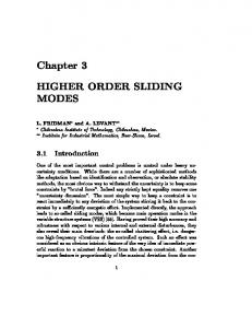
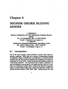
Higher-order sliding modes, differentiation and output ...

Levant A. Higher-order sliding modes, differentiation and output-feedback control. IJC,76(9/10),924-941,(2003)

Higher-order sliding modes, differentiation and output-feedback control Arie Levant School of Mathematical Sciences, Tel-Aviv University, Ramat-Aviv, 69978 Tel-Aviv, Israel E-mail: [email protected] . Tel.: 972-3-6408812, Fax: 972-3-6407543

Abstract. Being a motion on a discontinuity set of a dynamic system, sliding mode is used to keep accurately a given constraint and features theoretically-infinite-frequency switching. Standard sliding modes provide for finite-time convergence, precise keeping of the constraint and robustness with respect to internal and external disturbances. Yet the relative degree of the constraint has to be 1, and a dangerous chattering effect is possible. Higher order sliding modes preserve or generalize the main properties of the standard sliding mode and remove the above restrictions. r-sliding mode realization provides for up to the rth order of sliding precision with respect to the sampling interval compared with the first order of the standard sliding mode. Such controllers require higher-order real-time derivatives of the outputs to be available. The lacking information is achieved by means of proposed arbitrary-order robust exact differentiators with finite-time convergence. These differentiators feature optimal asymptotics with respect to input noises and can be used for numerical differentiation as well. The resulting controllers provide for the full output-feedback real-time control of any output variable of an uncertain dynamic system, if its relative degree is known and constant. The theoretical results are confirmed by computer simulation. 1

Introduction

Control under uncertainty condition is one of the main topics of the modern control theory. In spite of extensive and successful development of robust adaptive control and backstepping technique (Kokotovic and Arcak 2001, Landau et al. 1998) the sliding-mode control approach stays probably the main choice when one needs to deal with non-parametric uncertainties and unmodeled dynamics. That approach is based on keeping exactly a properly chosen constraint by means of high-frequency control switching. It exploits the main features of the sliding mode: its insensitivity to external and internal disturbances, ultimate accuracy and finite-time transient. However, the standard sliding-mode usage is bounded by some restrictions. The constraint being given by an 1


equality of an output variable s to zero, the standard sliding mode may be implemented only if the relative degree of s is 1. In other words, control has to appear explicitly already in the first total derivative s& . Also, high frequency control switching leads to the so-called chattering effect which is exhibited by high frequency vibration of the controlled plant and can be dangerous in applications. A number of methods were proposed to overcome these difficulties. In particular, high-gain control with saturation approximates the sign-function and diminishes the chattering, while on-line estimation of the so-called equivalent control (Utkin 1992) is used to reduce the discontinuouscontrol component (Slotine and Li 1991), the sliding-sector method (Furuta and Pan 2000) is suitable to control disturbed linear time-invariant systems. Yet, the sliding-mode order approach (Levantovsky 1985, Levant 1993) seems to be the most comprehensive, for it allows to remove all the above restrictions, while preserving the main sliding-mode features and improving its accuracy. Independently developed dynamical (Sira-Ramírez 1993, Rios-Bolívar et al. 1997) and terminal (Man et al. 1994) sliding modes are closely related to this approach. Suppose that s º 0 is kept by a discontinuous dynamic system. While successively differentiating s along trajectories, a discontinuity will be encountered sooner or later in the general case. Thus, sliding modes s º 0 may be classified by the number r of the first successive (r)

total derivative s which is not a continuous function of the state space variables or does not exist due to some reason like trajectory nonuniqueness. That number is called sliding order (Levant 1993, Fridman and Levant 1996, Bartolini et al. 1999a). The standard sliding mode on which most variable structure systems (VSS) are based is of the first order ( s& is discontinuous). While the standard modes feature finite time convergence, convergence to higher order sliding modes (HOSM) may be asymptotic as well. While the standard sliding mode precision is proportional to the time interval between the measurements or to the switching delay, r-sliding mode realization may provide for up to the rth order of sliding precision with respect to the measurement interval (Levant 1993). Properly used, HOSM totally removes the chattering effect. Trivial cases of asymptotically stable HOSM are often found in standard VSSs. For example there is an asymptotically stable 2-sliding mode with respect to the constraint x = 0 at the origin x = x& = 0 (at one point only) of a 2-dimensional VSS keeping the constraint x + x& = 0 in a standard 1-sliding mode. Asymptotically stable or unstable HOSMs inevitably appear in VSSs with 2


fast actuators (Fridman 1990, Fridman and Levant 1996, 2002). Stable HOSM leads in that case to spontaneous disappearance of the chattering effect. Asymptotically stable or unstable sliding modes of any order are well known (Emelyanov et al. 1986, Elmali and Olgac 1992, Fridman and Levant 1996). Dynamic sliding modes (Sira-Ramírez 1993, Spurgeon and Lu 1997) produce asymptotically stable higher-order sliding modes and are to be specially mentioned here. A family of finite-time convergent sliding mode controllers is based on so-called “terminal sliding modes” (Man et al. 1994, Wu et al. 1998). Having been independently developed, the first version of these controllers is close to the so-called “2-sliding algorithm with a prescribed convergence law” (Emelyanov et al. 1986, Levant 1993). The latter version is intended actually to provide for arbitrary-order sliding mode with finite-time convergence. Unfortunately, the resulting closed-loop systems have unbounded right-hand sides, which prevents the very implementation of the Filippov theory. Thus, such a mode cannot be considered as HOSM. The corresponding control is formally bounded along each transient trajectory, but takes on infinite values in any vicinity of the steady state. In order to avoid infinite control values all trajectories are to start from a prescribed sector of the state space. The very definition and the existence of the solution require some special study here. Arbitrary-order sliding controllers with finite-time convergence were only recently demonstrated (Levant 1998b, 2001a). The proofs of these results are for the first time published in the present paper. These controllers provide for full output control of uncertain Single-InputSingle-Output (SISO) weakly-minimum-phase dynamic systems with a known constant relative degree r. The control influence is a discontinuous function of the output and its r-1 real-timecalculated successive derivatives. The controller parameters may be chosen in advance, so that only one parameter is to be adjusted in order to control any system with a given relative degree. No detailed mathematical model is needed. The system’s relative degree being artificially increased, sliding control of arbitrary smoothness order can be achieved, completely removing the chattering effect. Since many mechanical systems have constant relative degree due, actually, to the Newton law, the application area for these controllers is very wide. Any implementation of the above controllers requires real-time robust estimation of the higher-order total output derivatives. The popular high-gain observers (Dabroom and Khalil 1997) would destroy the exactness and finite-time-convergence features of the proposed controllers. The 3


first-order robust exact differentiator (Levant 1998a) can be used here, but its successive application is cumbersome and not effective. The proposed lth-order differentiator allows real-time robust exact differentiation up to the order l, provided the next (l+1)th input derivative is bounded. Its performance is proved to be asymptotically optimal in the presence of small Lebesguemeasurable input noises. This paper is the first regular publication of these differentiators and of the corresponding proofs. Their features allow broad implementation in the nonlinear feedback control theory due to the separation principle (Atassi and Khalil 2000) triviality. They can be also successfully applied for numerical differentiation. The rth-order sliding controller combined with the (r-1)th-order differentiator produce an output-feedback universal controller for SISO processes with permanent relative degree (Levant 2002). Having been only recently obtained, the corresponding results are only briefly described in this paper, for the author intends to devote a special paper to this subject. The features of the proposed universal controllers and differentiators are illustrated by computer simulation. 2.

Preliminaries: higher-order sliding modes

Let us recall first that according to the definition by Filippov (1988) any discontinuous n

differential equation x& = v ( x ) , where x Î R and v is a locally bounded measurable vector function, is replaced by an equivalent differential inclusion x& Î V(x). In the simplest case, when v is continuous almost everywhere, V(x) is the convex closure of the set of all possible limits of v(y) as y ® x, while {y} are continuity points of v. Any solution of the equation is defined as an absolutely continuous function x(t), satisfying the differential inclusion almost everywhere. In the following the equation x& = v ( x ) can be considered as a result of closing a smooth dynamic system by some possibly-dynamical discontinuous feedback. Let s(x) be a smooth scalar output function. Then, provided that successive total time (r-1)

derivatives s, s& , ..., s

are continuous functions of the closed-system state space variables, and

the r-sliding point set (Figure 1) && = ... = s s = s& = s

(r-1)

= 0.

(1)

is non-empty and consists locally of Filippov trajectories, the motion on set (1) is called r-sliding mode (rth-order sliding mode, Levantovsky 1985, Levant 1993, Fridman and Levant 1996). The additional condition of the Filippov velocity set V containing more than 1 vector may (r)

be imposed in order to exclude some trivial cases. It is natural to call the sliding order r strict if s 4


is discontinuous or does not exist in a vicinity of the r-sliding point set, but sliding-mode orders are mostly considered strict by default.

Figure 1. 2-sliding mode Hence, r-sliding modes are determined by equalities (1) which impose an r-dimensional condition on the state of the dynamic system. The sliding order characterizes the dynamics smoothness degree in some vicinity of the sliding mode. && , ..., s Suppose that s, s& , s

(r-1)

are differentiable functions of x and that

rank[Ñs, Ñ s& ,..., Ñs

(r-1)

] = r.

(2)

Equality (2) together with the requirement for the corresponding derivatives of s to be differentiable functions of x is referred to as r-sliding regularity condition. If regularity condition (2) holds, then the r-sliding set is a differentiable manifold and s, s& , ..., s

(r-1)

may be

supplemented up to new local coordinates. Proposition 1 (Fridman and Levant 1996). Let regularity condition (2) be fulfilled and r-sliding manifold (1) be non-empty. Then an r-sliding mode with respect to the constraint function s exists if and only if the intersection of the Filippov vector-set field with the tangential space to manifold (1) is not empty for any r-sliding point. Proof. The intersection of the Filippov set of admissible velocities with the tangential space to the sliding manifold (1) induces a differential inclusion on this manifold (Figure 1). This inclusion satisfies all the Filippov conditions for solution existence. Therefore manifold (1) is an integral one. n A sliding mode is called stable if the corresponding integral sliding set is stable. The above definitions are easily extended to include the non-autonomous case by introduction of the fictitious equation t& =1. Vector output s requires vector sliding order to be defined and is not considered here. 5


Real sliding. Up to this moment only ideal sliding modes were considered which keep s º 0. In reality, however, switching imperfections being present, ideal sliding cannot be attained. The simplest switching imperfection is discrete switching caused by discrete measurements. It was proved (Levant 1993) that the best possible sliding accuracy attainable with discrete switching in (r)

r

s is given by the relation |s| ~ t , where t > 0 is the minimal switching time interval. Moreover, (k)

r-k

|s | ~ t , k = 0, 1, .... r are satisfied at the same time (s

the relations

(0)

= s). Thus, in order to

achieve the rth order of sliding precision in discrete realization, the sliding mode order in the continuous-time VSS has to be at least r. The standard sliding modes provide for the first-order real sliding only. The second order of real sliding was achieved by discrete switching modifications of the 2-sliding algorithms (Levant 1993, Bartolini et al. 1998) and by a special discrete switching algorithm (Su et al. 1994). Real sliding of higher orders is demonstrated in (Fridman and Levant 1998, Levant 1998b, 2001a). In practice the final sliding accuracy is always achieved in finite time. When asymptotically stable modes are considered, however, it is not observable at any fixed moment, for the convergence time tends to infinity with the rise in accuracy. In the known cases the limit accuracy of the asymptotically stable modes can be shown to be of the first order only (Slotine and Li 1991). The above-mentioned highest precision is probably obtained only with finite-time-convergence sliding modes. 3.

The problem statement and its solutions with low relative degrees

Consider a dynamic system of the form x& = a(t,x) + b(t,x)u,

s = s(t, x),

(3)

n

where x Î R , u Î R, a, b, s are smooth unknown functions, the dimension n is also unavailable. The relative degree r of the system is assumed to be constant and known. The task is to fulfill the constraint s(t, x) = 0 in finite time and to keep it exactly by some feedback. Extend system (3) by introduction of a fictitious variable xn+1 = t, x& n +1 = 1 . Denote ae = t

t

(a,1) , be = (b,0) , where the last component corresponds to xn+1. The equality of the relative degree r-2

to r means that the Lie derivatives Lbes, LbeLaes, ..., LbeLae s equal zero identically in a vicinity of r-1

a given point and LbeLae s is not zero at the point (Isidori 1989).

6


In a simplified way the equality of the relative degree to r means that u first appears explicitly only in the rth total derivative of s. In that case regularity condition (2) is satisfied (r) (Isidori 1989) and ¶ s ¹ 0 at the given point. The output s satisfies an equation of the form ¶u

(r)

s = h(t,x) + g(t,x)u . (4) (r) r r-1 ¶ It is easy to check that g = LbeLae s = ¶u s , h = Lae s. Obviously, h is the rth total time derivative of s calculated with u = 0. In other words, unknown functions h and g may be defined using only input-output relations. The heavy uncertainty of the problem prevents immediate reduction of (3) to any standard form by means of standard approaches based on the knowledge of a, b and s. Nevertheless, the very existence of standard form (4) is important here. Proposition 2 (Fridman and Levant 1996). Let system (3) have relative degree r with respect to the output function s at some r-sliding point (t0, x0). Let, also, u=U(t,x), the discontinuous function U taking on values from sets [K,¥) and (-¥,-K] on some sets of non-zero measure in any vicinity of each r-sliding point near point (t0, x0). Then this provides, with sufficiently large K, for the existence of r-sliding mode in some vicinity of the point (t0, x0). Proof. Proposition 2 is a straight-forward consequence of Proposition 1 and equation (4). n The trivial controller u = - K sign s satisfies Proposition 2. Usually, however, such a mode is not stable. The r-sliding mode motion is described by the equivalent control method (Utkin 1992), on the other hand, this dynamics coincides with the zero-dynamics (Isidori 1989) of the corresponding systems. The problem is to find a discontinuous feedback u = U(t, x) causing the appearance of a finite-time convergent r-sliding mode in (3). That new controller has to generalize the standard 1-sliding relay controller u = - K sign s. Hence, g(t,y) and h(t,y) in (4) are assumed to be bounded, g > 0. Thus, it is required that for some Km, KM, C > 0 0 < Km £

¶ ¶u

(r)

s £ KM,

(r)

| s |u=0 | £ C.

(5)

2.1 Solutions of the problem with relative degrees r = 1, 2. In case r = 1 calculation shows that s& (t, x, u) = s¢t(t, x) + s¢x(t, x) a(t, x) + s¢x(t, x) b(t, x) u,

and the problem is easily solved by the standard relay controller u = - a sign s, with a > C/Km. Here h = s& |u=0 = s¢t + s¢x a is globally bounded and g = accuracy with respect to the sampling interval is ensured . 7

¶ ¶u

s& = s¢xb. The first-order real-sliding


Let r = 2. The following list includes only few most known controllers. The so-called twisting controller (Levantovsky 1985, Emelyanov et al. 1986, Levant 1993) and the convergence conditions are given by u = - (r1 sign s + r2 sign s& ), r1 > r2 > 0, (r1 + r2)Km - C > (r1 - r2)KM + C, (r1 - r2)Km > C. (6) A particular case of the controller with prescribed convergence law (Emelyanov et al. 1986, Levant 1993) is given by 1/2

2

u = - a sign( s& + l|s| sign s), a, l > 0, aKm - C > l /2.

(7)

Controller (7) is close to terminal sliding mode controllers (Man et al. 1994). The so-called suboptimal controller (Bartolini et al. 1998, 1999a, b) is given by u = - r1 sign (s - s*/2) + r2 sign s*,

r1 > r2 > 0,

(8)

2[(r1 + r2)Km - C ] > (r1 - r2)KM + C, (r1 - r2)Km > C,

(9)

where s* is the current value of s detected at the closest time when s& was 0. The initial value of s* is 0. Any computer implementation of this controller requires successive measurements of s& or s with some time step. Usually the detection of the moments when s& changes its sign is performed. The control value u depends actually on the history of s& and s measurements, i.e. on s& (×) and s(×). Theorem 1 (Levant 1993, Bartolini et al. 1998). 2-sliding controllers (6), (7), (8) provide for finitetime convergence of any trajectory of (3), (5) to 2-sliding mode s º 0. The convergence time is a locally bounded function of the initial conditions. Let the measurements be carried out at times ti with constant step t > 0, si = s(ti, x(ti)), Dsi = si 1/2

- si-1, t Î [ti, ti+1). Substituting si for s , sign Dsi for sign s& , and sign(Dsi - lt|si| sign si) for 1/2

sign( s& - l|s| sign s) achieve discrete-sampling versions of the controllers. Theorem 2 (Levant 1993, Bartolini et al. 1998). Discrete-sampling versions of controllers (6), (7), 2

(8) provide for the establishment of the inequalities |s| < m0t , | s& | < m1t for some positive m0, m1. All listed controllers may be used also with relative degree 1 in order to remove the chattering and improve the sliding accuracy. Indeed, let u = j(s(×), s& (×)) be one of controllers (6), (7), (8), depending possibly on the previous measurements as in (8), then under certain natural conditions (Levant 1993, Bartolini et al. 1999a) the controller u = - sign s can be replaced by the controller u& = - u with |u| > 1, u& = j(s(×), s& (×)) with |u| £ 1.

Consider the general case. Let u be defined from the equality 8


d dt

where Pr-1(l) = l

(r-1)

+ a1l

(r-2)

[Pr-1( dtd )s] = - sign [Pr-1( dtd )s],

+ ... + ar-1 is a stable polynomial, aiÎR. In the case r = 1, P0 = 1

achieve the standard 1-sliding mode. Let r > 1. The r-sliding mode exists here at the origin and is asymptotically stable. There is also a 1-sliding mode on the manifold Pr-1( dtd )s = 0. Trajectories transfer in finite time into the 1-sliding mode on the manifold Pr-1( dtd )s = 0 and then exponentially converge to the r-sliding mode. Dynamic-sliding-mode controllers (Sira-Ramírez 1993, Spurgeon and Lu 1997) are based on such modes. Unfortunately, due to the dependence on higher-order derivatives of s the control is not bounded here even with small s. Also the accuracy here is the same as of the 1-sliding mode.

4.

Building an arbitrary-order sliding controller

Let p be any positive number, p ³ r. Denote N1,r = |s|

(r- 1)/ r p/r

, p/(r-1)

Ni,r = (|s| + | s& | p/r

p/(r-1)

Nr-1,r = (|s| + | s& |

(i-1) p/( r-i+1) (r- i)/p

+ ... + |s

+ ... + |s

|

)

, i = 1,..., r-1,

(r-2) p/2 1/p

|

) .

f0,r = s, f1,r = s& + b1 N1,r sign(s), (i)

fi,r = s + bi Ni,r sign(fi-1,r ), i = 1,..., r-1, where b1,..., br-1 are positive numbers. Theorem 3 (Levant 1998a, 2001). Let system (3) have relative degree r with respect to the output function s and (5) be fulfilled. Suppose also that trajectories of system (3) are infinitely extendible in time for any Lebesgue-measurable bounded control. Then with properly chosen positive parameters b1,..., br-1, a the controller

& , ..., s u = - a sign(fr-1,r(s, s

(r-1)

))

(10)

leads to the establishment of an r-sliding mode s º 0 attracting each trajectory in finite time. The convergence time is a locally bounded function of initial conditions. The proof of Theorem 3 is given in Appendix 1. It is the first publication of the proof. The assumption on the solution extension possibility means in practice that the system be weakly minimum phase. The positive parameters b1,..., br-1 are to be chosen sufficiently large in the index order. They determine a controller family applicable to all systems (3) of relative degree r 9


satisfying (5) for some C, Km, KM. Parameter a > 0 is to be chosen specifically for any fixed C, Km, KM. The proposed controller may be generalized in many ways. For example, coefficients of Ni,r may be any positive numbers, (10) can be smoothed (Levant 1999). Certainly, the number of choices of bi is infinite. Here are a few examples with bi tested for r £ 4, p being the least common multiple of 1, 2, ..., r. The first is the relay controller, the second coincides with (7). 1. u = - a sign s, 2. u = - a sign( s& + |s| sign s), 1/2

&& + 2 (| s& | +|s| ) 3. u = - a sign( s 3

2 1/6

sign( s& + |s| sign s)),

&& + s& +|s| ) 4. u = - a sign{ &&& s +3 ( s 6

4

2/3

3 1/12

&& + ( s& +|s| ) sign( s& +0.5 |s| sign s )]}, sign[ s 4

& | + |s && | + | &&& s| ) 5. u = -a sign(s + b4 (|s| + | s (4)

15

12

&& | ) |s

20 1/30

20

30 1/60

3 1/6

3/4

sign( &&& s +b3 (|s| + | s& | + 12

&& + b2(|s| + | s& | ) sign( s 12

Obviously, parameter a is to be taken negative with

15 1/20

¶ ¶u

15

& +b1|s| sign( s

4/5

sign s ))))

(r)

s < 0. Controller (10) is certainly

insensitive to any disturbance which keeps the relative degree and (5). No matching condition having been supposed, the residual uncertainty reveals itself in the r-sliding motion equations (in other words, in zero dynamics).

Figure 2. The idea of the r-sliding controller

Figure 3. The 3-sliding controller discontinuity set

The idea of the controller is that a 1-sliding mode is established on the smooth parts of the discontinuity set G of (10) (Figures 2, 3). That sliding mode is described by the differential equation fr-1,r = 0 providing in its turn for the existence of a 1-sliding mode fr-2,r = 0. But the primary sliding mode disappears at the moment when the secondary one is to appear. The resulting movement takes place in some vicinity of the cylindrical subset of G satisfying fr-2,r = 0, transfers

10


in finite time into some vicinity of the subset satisfying fr-3,r = 0 and so on. While the trajectory

& , ..., s approaches the r-sliding set, set G retracts to the origin in the coordinates s, s

(r-1)

& , ..., s Controller (10) requires the availability of s, s

(r-1)

.

. That information demand may be

lowered. Let the measurements be carried out at times ti with constant step t > 0. Consider the controller u(t) = -a sign(Dsi (j)

(j)

(r-2)

+ br-1t Nr-1,r (si, s& i ,...,si

where si = s (ti, x(ti)), Dsi

(r-2)

(r-2)

(r-2)

= si

- si-1

(r-2)

)sign(fr-2,r(si, s& i ,...,si

(r-2)

))),

(11)

, t Î [ti, ti+1).

Theorem 4 (Levant 1998b, 2001a). Under conditions of Theorem 1 with discrete measurements both algorithms (10) and (11) provide in finite time for fulfillment of the inequalities |s| < a0t , | s& | < a1t , ..., |s r

r-1

(r-1)

| < ar-1t

for some positive constants a0, a1, ..., ar-1. The convergence time is a locally bounded function of initial conditions. That is the best possible accuracy attainable with discontinuous s

(r)

separated from zero

(Levant 1993). The proof of Theorem 4 is given in Appendix 1. Following are some remarks on the usage of the proposed controllers. Convergence time may be reduced increasing the coefficients bj. Another way is to substitute -j (j)

l s

(j)

r

for s , l a for a and lt for t in (10) and (11), l > 1, causing convergence time to be

diminished approximately by l times. As a result the coefficients of Ni, r will differ from 1. Local application of the controller. In practical applications condition (5) is often globally invalid. Nevertheless, it usually holds in some restricted area of the state space containing the actual region of the system operation. In fact, that is always true, if the constraint keeping problem is well posed from the engineering point of view. The practical implementation of the controller is straightforward in that case and is based on the following simple Proposition proved in Appendix 1. Proposition 3. Under the conditions of Theorem 3, for any RM > 0 there exists such Rm, RM > Rm > 0, that any trajectory starting in the disk of radius Rm which is centered at the origin of the space

& , ..., s s, s

(r-1)

does not leave the larger disk of the radius RM while converging to the origin.

Moreover, RM - Rm and the maximal convergence time can be made arbitrarily small choosing b1,..., br-1, a sufficiently large in the list order. Implementation of r-sliding controller when the relative degree is less than r. Let the relative (r-k-1)

degree k of the process be less than r. Introducing successive time derivatives u, u& , ..., u 11

as

Levant A. Higher-order sliding modes, differentiation and output-feedback control. IJC,76(9/10),924-941,(2003) (r-k)

new auxiliary variables and u

as a new control, achieve a system of the relative degree r.

Condition (5) is locally satisfied for the new control. The standard r-sliding controller may be now locally applied. The resulting control u(t) is an (r-k-1)-smooth function of time with k < r - 1, a Lipschitz function with k = r - 1 and a bounded “infinite-frequency switching” function with k = r. A global controller was developed by Levant (1993) for r = 2, k = 1. (r-1)

Chattering removal. The same trick removes the chattering effect. For example, substituting u

for u in (10), receive a local r-sliding controller to be used instead of the relay controller u = - sign s and attain the rth-order sliding precision with respect to t by means of an (r - 2)-times differentiable control with a Lipschitzian (r-2)th time derivative. It has to be modified like in (Levant 1993) in order to provide for the global boundedness of u and global convergence. Controlling systems nonlinear on control. Consider a system x& = f(t,x,u) nonlinear on control. Let ¶ s(i)(t,x,u) = 0 for i = 1, ..., r-1, ¶ s(r)(t,x,u) > 0. It is easy to check that ¶u ¶u s

(r+1)

r+1

= Lu s +

¶ ¶u

s

(r)

u& , Lu(×) =

¶ ¶t

(×) +

¶ ¶x

(×) f(t,x,u).

The problem is now reduced to that considered above with relative degree r+1 by introducing a new auxiliary variable u and a new control v = u& . Real-time control of output variables. The implementation of the above-listed r-sliding controllers && , ..., s requires real-time observation of the successive derivatives s& , s

(r-1)

. In case system (3) is

known and the full state is available, these derivatives may be directly calculated. In the real uncertainty case the derivatives are still to be real-time evaluated in some way. Thus, one would not theoretically need to know any model of the controlled process, only the relative degree and 3 constants from (5) were needed in order to adjust the controller. Unfortunately, the problem of successive real-time exact differentiation is usually considered as practically insoluble. (r)

Nevertheless, as is shown in the next Section, the boundedness of s , which follows from (4), (5) && , ..., s allows robust exact estimation of s& , s

(r-1)

in real time.

5 Arbitrary-order exact robust differentiator Real-time differentiation is an old and well-studied problem. The main difficulty is the obvious differentiation sensitivity to input noises. The popular high-gain differentiators (Atassi and Khalil 2000) provide for an exact derivative when their gains tend to infinity. Unfortunately, at the same time their sensitivity to small high-frequency noises also grows infinitely. With any finite gain values such a differentiator has also a finite bandwidth. Thus, being not exact, it is, at the same time, 12


insensitive with respect to high-frequency noises. Such insensitivity may be considered both as advantage or disadvantage depending on the circumstances. Another drawback of the high-gain differentiators is their peaking effect: the maximal output value during the transient grows infinitely when the gains tend to infinity. The main problem of the differentiator feedback application is the so-called separation problem. The separation principle means that a controller and an observer (differentiator) can be designed separately, so that the combined observer-controller output feedback preserve the main features of the controller with the full state available. The separation principle was proved for asymptotic stabilization of feedback-linearizable systems with high-gain observers (Atassi and Khalil 2000, Isidori et al. 2000). That important result is realized in spite of the non-exactness of high-gain observers with any fixed finite gain values. The qualitative explanation is that the output derivatives of all orders vanish during the continuous-feedback stabilization. Thus, the frequency of the signal to be differentiated also vanishes, and the differentiator provides for asymptotically exact (r)

derivatives. On the contrary, in the case considered in the previous section s

is chattering with a

finite magnitude and a frequency tending to infinity while approaching the r-sliding mode. Thus, the signal s is problematic for a high-gain differentiator. Indeed, the closer to the r-sliding mode, the higher gain is needed to produce a good derivative estimation of s

(r-1)

. As a result, convergence into

some vicinity of the r-sliding mode could only be attained. The sliding-mode differentiators (Golembo et al. 1976, Yu et al. 1996) also do not provide for exact differentiation with finite-time convergence due to the output filtration. The differentiator by Bartolini et al. (2000) is based on a 2-sliding-mode controller using the real-time measured sign of the derivative to be calculated. Therefore, the first finite difference of the differentiator input is used with the sampling step proportional to the square root of the maximal noise magnitude. That is rather inconvenient and requires possibly-lacking information on the noise. Exact derivatives may be calculated by successive implementation of a robust exact firstorder differentiator (Levant 1998a) with finite-time convergence. That differentiator is based on 2sliding mode and is proved to feature the best possible asymptotics in the presence of infinitesimal Lebesgue-measurable measurement noises, if the second time derivative of the unknown base 1/2

signal is bounded. The accuracy of that differentiator is proportional to e , where e is the maximal measurement-noise magnitude and is also assumed to be unknown. Therefore, having been n times 13


successively implemented, that differentiator will provide for the nth-order differentiation accuracy -n (2 )

of the order of e

. Thus, the differentiation accuracy deteriorates rapidly. On the other hand, it is

proved by Levant (1998a) that when the Lipschitz constant of the nth derivative of the unknown clear-of-noise signal is bounded by a given constant L, the best possible differentiation accuracy of i/(n+1) (n+1-i)/(n+1)

e

the ith derivative is proportional to L

, i = 0, 1, ..., n. Therefore, a special

differentiator is to be designed for each differentiation order. Let input signal f(t) be a function defined on [0, ¥) consisting of a bounded Lebesguemeasurable noise with unknown features and an unknown base signal f0(t) with the nth derivative having a known Lipschitz constant L > 0. The problem is to find real-time robust estimations (n) of f& (t), &f& (t), ... , f (t) being exact in the absence of measurement noises. 0

0

0

Two similar recursive schemes of the differentiator are proposed here. Let an (n-1)th-order i differentiator D (f(×), L) produce outputs D , i = 0, 1, ..., n - 1, being estimations of f , f& , &f& , n-1

..., f0

(n-1)

0

n-1

for any input f(t) with f0

(n-1)

0

0

having Lipschitz constant L > 0. Then the nth-order

i

differentiator has the outputs zi = Dn , i = 0, 1, ..., n, defined as follows: z& 0 = v ,

v = -l0 | z0 - f(t)| 0

n/( n + 1)

z1 = Dn-1 (v(×), L), ..., zn = Dn-1

n-1

sign(z0 - f(t)) + z1,

(12)

(v(×), L).

Here D0(f(×), L) is a simple nonlinear filter D0: z& = -l sign(z - f(t)),

l > L.

(13)

Thus, the first-order differentiator coincides here with the above-mentioned differentiator (Levant 1998a) : z& 0 = v ,

v = -l0 | z0 - f(t)|

1/2

sign(z0 - f(t)) + z1,

z& 1 = -l1 sign(z1 - v) = -l1 sign(z0 - f(t)).

(14)

Another recursive scheme is based on the differentiator (14) as the basic one. Let ~ ~ Dn -1 (f(×), L) be such a new (n-1)th-order differentiator, n ³ 1, D1 (f(×), L) coinciding with the differentiator D1(f(×), L) given by (14). Then the new scheme is defined as z& 0 = v , v = -l0 | z0 - f(t)|

n/( n + 1)

sign(z0 - f(t)) + w0 + z1 ,

(n - 1)/( n +1)

w& 0 = -a0 | z0 - f(t)|

sign(z0 - f(t));

~ ~ z1 = Dn0-1 (v(×), L), ..., zn = Dnn--11 (v(×), L). 14

(15)


The resulting 2nd-order differentiator (Levant 1999) is as follows: z& 0 = v0, v0 = -l0 | z0 - f(t)| 1/3

w& 0 = -a0 | z0 - f(t)|

2/3

sign(z0 - f(t)) + w0 + z1,

sign(z0 - f(t));

z& 1 = v1 , v1 = -l1 | z1 - v0|

1/2

sign(z1 - v0) + w1,

w& 1 = -a1 sign(z1 - v0); z2 = w1.

Similarly, a 2nd-order differentiator from each of these sequences may be used as a base for a new recursive scheme. An infinite number of differentiator schemes may be constructed in this way. The only requirement is that the resulting systems be homogeneous in a sense described further. While the author has checked only the above two schemes (12), (13) and (14), (15), the conjecture is that all such schemes produce working differentiators, provided suitable parameter choice. Differentiator (12) takes on the form z& 0 = v0 ,

v0 = -l0 | z0 - f(t)|

z& 1 = v1 ,

v1 = -l1 | z1 - v0|

n/( n + 1)

(n-1)/ n

sign(z0 - f(t)) + z1,

sign(z1 - v0) + z2,

...

(16)

z& n-1 = vn-1 , vn-1 = -ln-1 | zn-1 - vn-2|

1/ 2

sign(zn-1 - vn-2) + zn,

z& n = -ln sign(zn - vn-1). Theorem 5. The parameters being properly chosen, the following equalities are true in the absence of input noises after a finite time of a transient process: z0 = f0(t);

(i)

zi = vi-1 = f0 (t), i = 1, ..., n.

Moreover, the corresponding solutions of the dynamic systems are Lyapunov stable, i.e. (i)

finite-time stable (Rosier 1992). The Theorem means that the equalities zi = f0 (t) are kept in 2sliding mode, i = 0, ..., n-1. Here and further all Theorems are proved in Appendix 2. Theorem 6. Let the input noise satisfy the inequality |f(t) - f0(t)| £ e. Then the following inequalities are established in finite time for some positive constants mi, ni depending exclusively on the parameters of the differentiator: (i)

(n - i +1)/(n + 1)

|zi - f0 (t)| £ mi e |vi - f0

(i+1)

, i = 0, ..., n;

(n - i )/(n + 1)

(t)| £ ni e

, i = 0, ..., n-1.

Consider the discrete-sampling case, when z0(tj) - f(tj) is substituted for z0 - f(t) with tj £ t < tj+1, tj+1 - tj = t > 0. 15


Theorem 7. Let t > 0 be the constant input sampling interval in the absence of noises. Then the following inequalities are established in finite time for some positive constants mi, ni depending exclusively on the parameters of the differentiator: (i)

|zi - f0 (t)| £ mi t |vi - f0

n-i+1

(i+1)

(t)| £ ni t

n-i

, i = 0, ..., n; , i = 0, ..., n - 1.

In particular, the nth derivative error is proportional to t. The latter Theorem means that there are a number of real sliding modes of different orders. Nevertheless, nothing can be said on the derivatives of vi and of z& i, because they are not continuously differentiable functions. Homogeneity of the differentiators. The differentiators are invariant with respect

to the

transformation n+1

(t, f, zi, vi, wi ) a ( ht, h

f, h

n-i+1

n-i

n-i

zi, h vi, h wi).

The parameters ai, li are to be chosen recursively in such a way that a1, l1, ..., an, ln provide for the convergence of the (n-1)th order differentiator with the same Lipschitz constant L, and a0, l0 be sufficiently large (a0 is chosen first). The best way is to choose them by computer simulation. A choice of the 5th-order differentiator parameters with L = 1 is demonstrated in Section 7. Recall that it contains parameters of all lower-order differentiators. Substituting f(t)/L for f(t) and taking new coordinates z¢i = L zi, v¢i = L vi, w¢i = L wi achieve the following proposition. Proposition 4. Let parameters a0i, l0i, i = 0, 1, ...., n, of differentiators (12), (13) or (14), (15) provide for exact n-th order differentiation with L = 1. Then the parameters ai = a0i L l0i L

1/(n-i+1)

(i)

are valid for any L > 0 and provide for the accuracy |zi - f0 (t)| £ miL

2/(n-i+1)

,

li =

i/(n + 1) (n - i +1)/(n + 1)

e

for some mi ³ 1. The separation principle is trivially fulfilled for the proposed differentiator. Indeed, the differentiator being exact, the only requirements for its implementation are the boundedness of some higher-order derivative of its input and the impossibility of the finite-time escape during the differentiator transient. Hence, the differentiator may be used in almost any feedback. Mark that the differentiator transient may be made arbitrarily short by means of the parameter transformation from Proposition 4, and the differentiator does not feature peaking effect (see the proof of Theorem 5 in Appendix 2).

16


Remarks. It is easy to see that the kth order differentiator provides for a much better accuracy of the lth derivative, l < k, than the lth order differentiator (Theorem 6). A similar idea is realized to improve the first derivative by Krupp et al. (2001). It is easy to check that after exclusion of the variables vi differentiator (16) may be rewritten in the non-recursive form z& 0 = -k0 | z0 - f(t)|

n/( n + 1)

sign(z0 - f(t)) + z1,

... z& i = -ki | z0 - f(t)|

(n - i)/( n + 1)

sign(z0 - f(t)) + zi+1,

i = 1, ..., n-1

... z& n = -kn sign(z0 - f(t)) for some positive ki calculated on the basis of l0, ..., ln. 6. Universal output-feedback SISO controller The results of this Section have been just recently obtained (Levant 2002), and the author supposes to describe them in a special paper. Thus, only a brief description is provided. Consider uncertain system (3), (5). Combining controller (10) and differentiator (16) achieve a combined Single-Input-Single-Output (SISO) controller u = - a sign(fr-1,r(z0, z1, ..., zr-1)), 1/r

z&0 = v0,

v0 = - l0,0 L

z&1 = v1,

v1 = - l0,1 L

| z0 - s|

1/(r-1)

(r-1)/r

| z1 - v0|

sign(z0 - s) + z1,

(r-2)/(r-1)

sign(z1 - v0) + z2,

... z&r -2 = vr-2,

vr-2 = - l0, r-2 L

1/2

| zr-2 - vr-3|

1/2

sign(zr-2- vr-3)+ zr-1,

z&r -1 = - l0, r-1 L sign(zr-1 - vr-2), where parameters li = l0, i L

1/(r- I)

(r)

of the differentiator are chosen according to the condition |s | £

L, L ³ C + aKM. In their turn, parameters l0i are chosen in advance for L = 1 (Proposition 4). Thus, parameters of controller (10) are chosen separately of the differentiator. In case when C and KM are known, only one parameter a is really needed to be tuned, otherwise both L and a might be found in computer simulation. Theorems 3, 4 hold also for the combined output-feedback controller. In particular, under the conditions of Theorem 3 the combined controller provides for the global

17


convergence to the r-sliding mode s º 0 with the transient time being a locally bounded function of the initial conditions. On the other hand, let the initial conditions of the differentiator belong to some compact set.

& , ..., s Than for any 2 embedded disks centered at the origin of the space s, s

(r-1)

the parameters of

the combined controller can be chosen in such a way that all trajectories starting in the smaller disk do not leave the larger disk during their finite-time convergence to the origin. The maximal convergence time can be made arbitrarily small. That allows for the local controller application. With discrete measurements, in the absence of input noises, the controller provides for the r

rth-order real sliding sup|s| ~ t , where t is the sampling interval. Therefore, the differentiator does not spoil the r-sliding asymptotics if the input noises are absent. It is also proved that the resulting controller is robust and provides for the accuracy proportional to the maximal error of the input measurement (the input noise magnitude). Note once more that the proposed controller does not require detailed mathematical model of the process to be known. 7.

Simulation examples

7.1 Numeric differentiation Following are equations of the 5th-order differentiator with simulation-tested coefficients for L = 1: z& 0 = v0 , v0 = - 12 | z0 - f(t)| 4/5

z& 1 = v1 , v1

= - 8 | z1 - v0|

z& 2 = v2 , v2

= - 5 | z2 - v1|

z& 3 = v3 ,

= -3 | z3 - v2|

z& 4 = v4 ,

v3 v4

5/6

sign(z1 - v0) + z2 ,

3/4

2/3

= -1.5 | z4 - v3|

sign(z0 - f(t)) + z1 ,

(17) (18)

sign(z2 - v1) + z3 ,

(19)

sign(z3 - v2) + z4 ,

(20)

1/2

sign(z4 - v3) + z5 ,

z& 5 = -1.1 sign(z5 - v4);

(21) (22)

18


The differentiator parameters can be easily changed, for it is not very sensitive to their values. The tradeoff is as follows: the larger the parameters, the faster the convergence and the higher sensitivity to input noises and the sampling step. As mentioned, differentiator (17) - (22) contains also differentiators of the lower orders. For example, according to Proposition 4, the second order differentiator for the input f with | &f&& | £ L takes on the form z& 0 = v0 , z& 1 = v1 ,

v0 v1

1/3

= -3 L | z0 - f| = -1.5 L

1/2

2/3

sign(z0 - f) + z1 ,

| z 1 - v0 |

1/2

sign(z1 - v0) + z2 ,

z& 2 = -1.1 L sign(z2 - v1). Differentiator (17) - (22) and its 3rd-order sub-differentiator (19) - (22) (differentiating here the internal variable v1) were used for simulation. Initial values of the differentiator state were taken zero with exception for the initial estimation z0 of f, which is taken equal to the initial measured value of f. The base input signal f0(t ) = 0.5 sin 0.5t + 0.5 cos t.

(23)

was taken for the differentiator testing. Derivatives of f0(t ) do not exceed 1 in absolute value. Third order differentiator. The measurement step t = 10 -12

-8

-3

was taken, noises are absent. The

-5

attained accuracies are 5.8×10 , 1.4×10 , 1.0×10 , 0.0031 for the signal tracking, the first, second -16

-11

and third derivatives respectively. The derivative tracking deviations changed to 8.3×10 , 1.8×10 , -7

-4

1.2×10 and 0.00036 respectively after t was reduced to 10 . That corresponds to Theorem 7. -16

-12

-10

-7

Fifth order differentiator. The attained accuracies are 1.1×10 , 1.29×10 , 7.87×10 , 5.3×10 , -4

2.0×10

and 0.014 for tracking the signal, the first, second, third, fourth and fifth derivatives -4

respectively with t = 10 (Figure 4a). There is no significant improvement with further reduction of t. The author wanted to demonstrate the 10th order differentiation, but found that differentiation

19


of the order exceeding 5 is unlikely to be performed with the standard software. Further calculations are to be carried out with precision higher than the standard long double precision (128 bits per number).

a.

Signal without noise

b. Noisy signal

Figure 4. Fifth order differentiation Sensitivity to noises. The main problem of the differentiation is certainly its well-known sensitivity to noises. As we have seen, even small computer calculation errors appear to be a considerable noise in the calculation of the fifth derivative. Recall that, when the nth derivative has the Lipschitz constant 1 and the noise magnitude is e, the best possible accuracy of the ith order differentiation, (n-i+1)/(n+1)

i £ n, is k(i,n) e

(Levant 1998a), where k(i,n) > 1 is a constant independent on the

differentiation realization. That is a minimax (worst case) evaluation. Since differentiator (17) (22) assumes this Lipschitz input condition, it satisfies this accuracy restriction as well (see also -6

Theorems 6, 7). In particular, with the noise magnitude e = 10 the maximal 5th derivative error 1/6

exceeds e

= 0.1. For comparison, if the successive first-order differentiation were used, the (2-5)

respective maximal error would be at least e

= 0.649 and some additional conditions on the

input signal would be required. Taking 10% as a border, achieve that the direct successive differentiation does not give reliable results starting with the order 3, while the proposed differentiator may be used up to the order 5. With the noise magnitude 0.01 and the noise frequency about 1000 the 5th-order differentiator produces estimation errors 0.00042, 0.0088, 0.076, 0.20, 0.34 and 0.52 for signal (23) and its 5 derivatives respectively (Figure 4b). The differentiator performance does not 20


significantly depend on the noise frequency. The author found that the second differentiation scheme (15) provides for slightly better accuracies.

7.2. Output-feedback control simulation Consider a simple kinematic model of car control (Murray and Sastry 1993) x& = v cos j, y& = v sin j, j& = v/l tan q, q& = u, where x and y are Cartesian coordinates of the rear-axle middle point, j is the orientation angle, v is the longitudinal velocity, l is the length between the two axles and q is the steering angle (Figure 5). The task is to steer the car from a given initial position to the trajectory y = g(x), while x, g(x) and y are assumed to be measured in real time. Note that the actual control here is q and q& = u is used as a new control in order to avoid discontinuities of q. Any practical implementation of the developed here controller would require some real-time coordinate transformation with q approaching ±p/2. Define s = y - g(x).

(24)

Figure 5. Kinematic car model Let v = const = 10 m/s, l = 5 m, g(x) = 10 sin(0.05x) + 5, x = y = j = q = 0 at t = 0. The relative degree of the system is 3 and the listed 3-sliding controller may be applied here. The resulting steering angle dependence on time is not sufficiently smooth (Levant 2001b), therefore the relative degree is artificially increased up to 4, u& having been considered as a new control. The 4-sliding controller from the list in Section 3 is applied now, a = 20 is taken. The following 3rd order differentiator was implemented: 21

Levant A. Higher-order sliding modes, differentiation and output-feedback control. IJC,76(9/10),924-941,(2003) 3/4

z& 0 = v0 , v0

= - 25 | z0 - s|

z& 1 = v1 ,

= - 25 | z1 - v0|

2/3

sign(z1 - v0) + z2 ,

(26)

= - 33 | z2 - v1|

1/2

sign(z2 - v1) + z3 ,

(27)

z& 2 = v2 ,

v1 v2

sign(z0 - s) + z1 ,

(25)

z& 3 = -500 sign(z3 - v2).

(28) (4)

The coefficient in (28) is large due to the large values of s , other coefficients were taken according to Proposition 4 and (17) - (22). During the first half-second the control is not applied in && and &s&& order to allow the convergence of the differentiator. Substituting z0, z1, z2 and z3 for s, s& , s

respectively, obtain the following 4-sliding controller: u = 0, 0 £ t < 0.5, 6

4

3 1/12

u = - 20 sign{z3 +3 (z2 + z1 +| z0| )

4

3 1/6

3/4

sign[z2+ (z1 +| z0| ) sign(z1+0.5 | z0| sign z0 )]}, t ³ 0.5.

a. Car trajectory

b. 4-sliding deviations

c. Differentiator convergence

d. Steering angle

Figure 6. 4-sliding car control

22

Levant A. Higher-order sliding modes, differentiation and output-feedback control. IJC,76(9/10),924-941,(2003) -4

The trajectory and function y = g(x) with the sampling step t = 10 are shown in Figure 6a. The integration was carried out according to the Euler method, the only method effective for && , &&& sliding-mode simulation. Graphs of s, s& , s s are shown in Figure 6b. The differentiators’ performance within the first 1.5 seconds is demonstrated in Figure 6c. The steering angle graph && | £ (actual control) is presented in Figure 6d. The sliding accuracies |s| £ 9.3×10 , | s& | £ 7.8×10 , | s -8

-5

s | £ 0.43 were attained with the sampling time step t = 10 . 6.6×10 , | &&& -4

-4

8. Conclusions and discussion of the obtained results Arbitrary-order real-time exact differentiation together with the arbitrary-order sliding controllers provide for full SISO control based on the input measurements only, when the only information on the controlled uncertain weakly-minimum-phase process is actually its relative degree. A family of r-sliding controllers with finite time convergence is presented for any natural number r, providing for the full real-time control of the output variable if the relative degree r of the dynamic system is constant and known. Whereas 1- and 2-sliding modes were used mainly to keep auxiliary constraints, arbitrary-order sliding controllers may be considered as general-purpose controllers. In case the mathematical model of the system is known and the full state is available, the real-time derivatives of the output variable are directly calculated, and the controller implementation is straightforward and does not require reduction of the dynamic system to any specific form. If boundedness restrictions (5) are globally satisfied, the control is also global and the input is globally bounded. Otherwise the controller is still locally applicable. In the uncertainty case a detailed mathematical model of the process is not needed. Necessary time derivatives of the output can be obtained by means of the proposed robust exact differentiator with finite-time convergence. The proposed differentiator allows real-time robust exact differentiation up to any given order l, provided the next (l+1)th derivative is bounded by a known constant. These features allow wide application of the differentiator in nonlinear control theory. Indeed, after finite time transient in the absence of input noises its outputs can be considered as exact direct measurements of the derivatives. Therefore, the separation principle is trivially true for almost any feedback. At the same time, in the presence of measurement noises the differentiation accuracy inevitably deteriorates rapidly with the growth of the differentiation order (Levant 1998a), and direct observation of the derivatives is preferable. The exact derivative 23


estimation does not require tending some parameters to infinity or to zero. Even when treating noisy signals, the differentiator performance only improves with the sampling step reduction. The resulting combined controller provides for extremely high tracking accuracy in the r

absence of noises. The sliding accuracy is proportional to t , t being a sampling period and r being the relative degree. That is the best possible accuracy with discontinuous rth derivative of the output (Levant, 1993). It may be further improved increasing the relative degree artificially, which produces arbitrarily smooth control and removes also the chattering effect. The proposed controllers are easily developed for any relative degree, at the same time most of the practically important problems in output control are covered by the cases when relative degree equals 2, 3, 4 and 5. Indeed, according to the Newton law, the relative degree of a spatial variable with respect to a force, being understood as a control, is 2. Taking into account some dynamic actuator, achieve relative degree 3 or 4. If the actuator input is required to be a Lipschitz function, the relative degree is artificially increased to 4 or 5. Recent results (Bartolini et al. 1999b) seem to allow the implementation of the developed controllers for general Multi-Input-MultiOutput systems.

Appendix 1: proofs of Theorems 3, 4 and Proposition 3 The general idea of the proofs is presented in Section 4 and is illustrated by Figures 2, 3. Preliminary notions. The following notions are needed to understand the proof. They are based on results by Filippov (1988). m Differential inclusion x& Î X(x), x Î R is called further Filippov inclusion if for any x

1. X(x) is a closed non-empty convex set; m

2. X(x) Ì {v Î R | ||v|| £ r(x)}, where r(x) is a continuous function; 3. the maximal distance of the points of X(x¢) from X(x) tends to zero when x¢ ® x. Recall that any solution of a differential inclusion is an absolutely continuous function satisfying the inclusion almost everywhere, and that any differential equation with a discontinuous right-hand side is understood as equivalent to some Filippov inclusion. m m m The graph of a differential inclusion x& Î X(x), x Î R is the set {(x,z) Î R ´ R | z Î X(x)}. A differential inclusion x& Î X¢(x) is called e-close to the Filippov inclusion x& Î X(x) in some region if any point of the graph of x& Î X¢(x) is distanced by not more than e from the graph 24


of x& Î X(x). It is known that within any compact region solutions of x& Î X¢(x) tend to some (m) solutions of x& Î X(x) uniformly on any finite time interval with e ® 0. In the special case x Î (m-1) X(x, x& , ..., x ), x Î R, which is considered in the present paper, the graph may be considered as m

(m)

a set from R´ R . An inclusion x

(m-1) Î X¢(x, x& , ..., x ) corresponding to the closed e-vicinity of

that graph is further called the e-swollen inclusion. It is easy to see that this is a Filippov inclusion. An e-swollen differential equation is the inclusion corresponding to the e-vicinity of the corresponding Filippov inclusion. Proof of Theorem 3. Consider the movement of a projection trajectory of (3), (10) in coordinates s, s& , ..., s

(r-1)

: (r) r (r) s = Lae s(t,x) + u ¶ s (t,x,u). ¶u

(29)

Taking into account (5) achieve a differential inclusion (r)

s Î [-C, C] + [Km, KM] u ,

(30)

which will be considered from now on instead of the real equality (29). The operations on sets are naturally understood here as sets of operation results for all possible combinations of the operand set elements. Control u is given by (10) or (11). A given point P is called here a discontinuity point of a given function, if for any point set N of zero measure and any vicinity O of P there are at least 2 different limit values of the function

&, when point p Î O \ N approaches P. Let G be the closure of the discontinuity set of sign(fr-1,r (s, s ..., s

(r-1)

)) or, in other words, of control (10).

Lemma 1. Set G partitions the whole space s, s& , ..., s satisfying fr-1,r (s,...,s

(r-1)

) > 0 and fr-1,r (s,...,s

(r-1)

(r-1)

into two connected open components

) < 0 respectively. Any curve connecting points

from different components has a non-empty intersection with G.

& , ..., s ) = 0, i = 1, ..., r-1. It may be rewritten in the form Proof. Consider any equation fi,r(s, s (i)

& , ...,s s = xi(s, s (i)

(i-1)

& , ...,s ) = -bi N i,r(s, s

(i-1)

& , ...,s ) sign(fi-1,r (s, s

(i-1)

)).

Let Si be the closure of the discontinuity set of sign fi,r, i = 0, ..., r-1, G = Sr-1, and S0 = {0}Ì R

& , ..., s and is, actually, a modification of the graph of (Figure 7). Each set Si lies in the space s, s (i)

& , ...,s s = xi(s, s (i)

(i-1)

).

25


Figure 7. Internal structure of the discontinuity set The Lemma is proved by the induction principle. Obviously, S0 partitions R into two open connected components. Let Si-1 divide the space R with coordinates s, s& , ..., s i

connected components W

+ i-1

and W

-

(i-1)

into two open

with fi-1,r > 0 and fi-1,r < 0 respectively. It is easy to see

i-1

(Figure 7) that Si = {s, s& , ..., s | |s | £ biNi,r(s, s& , ..., s (i)

(i)

(s = -bi Ni,r(s, s& , ..., s (i)

(i-1)

) & (s, s& , ..., s

)sign(fi-1,r(s, s& , ..., s

(i-1)

(i-1)

W i = {s, s& , ..., s | s > biNi,r(s, s& , ..., s +

(i)

(i)

(i-1)

(s > -bi Ni,r(s, s& , ..., s (i)

-

(i)

) & (s, s& , ..., s

(i)

(s < bi Ni,r(s, s& , ..., s (i)

(i-1)

) Ï Si-1)};

(i-1)

)ÎW

+ i-1)};

)Ú

) & (s, s& , ..., s

(i-1)

+

)) & (s, s& , ..., s

(i-1)

Considering the division of the whole space s, s& , ..., s (i)

) Î Si-1 Ú

)Ú

(i-1)

W i = {s, s& , ..., s | s < -bi Ni,r(s, s& , ..., s

(i-1)

(i)

(i-1)

)ÎW

i-1)}. (i)

(i)

in the sets |s | £ biNi,r , s < -biNi,r and

-

s > biNi,r it is easily proved that W i and W i are connected and open. n Consider the transformation Gn : (t, s, s& , ..., s

(r-1)

) a (nt, n s, n s& , ..., ns r

r-1

(j)

to see that this linear transformation complies with understanding s

(r-1)

). It is easy

as coordinates and as

derivatives as well. It is also easy to check that inclusion (30), (10) is invariant with respect to Gn, n > 0. That invariance implies that any statement invariant with respect to Gn is globally true if it is r true on some set E satisfying the condition U Gn E = R . That reasoning is called further n³0

“homogeneity reasoning“. For example, it is sufficient to prove the following Lemma only for trajectories with initial conditions close to the origin. Lemma 2. With sufficiently large a any trajectory of inclusion (30), (10) hits G in finite time. (r-1)

Proof. Obviously, it takes finite time to reach the region |s

| £ br-1Nr-1,r . It is also easy to check

that it takes finite time for any trajectory in a sufficiently small vicinity of the origin to cross the 26

Levant A. Higher-order sliding modes, differentiation and output-feedback control. IJC,76(9/10),924-941,(2003) (r-1)

entire region |s

| £ br-1Nr-1,r if no switching happens. Thus, according to Lemma 1 set G is also

encountered on the way. The homogeneity reasoning completes the proof. n Lemma 3. There is a 1-sliding mode on fr-1,r = 0 in the continuity points of fr-1,r with sufficiently large a. There is such a choice of bj that each differential equation fi,r = 0, i = 1, ..., r-1 provides for the existence of a 1-sliding mode in the space s, s& , ..., s

(i-1)

& , ..., s xi-1(s, s

(i-2)

(i-1)

on the manifold s

=

) in continuity points of xi-1.

Proof. It is needed to prove that j& r -1,r sign fr-1,r < const < 0 with fr-1,r = 0 on trajectories of (30),

(10). The second statement means that for each i = 1, ..., r-1 the inequalities j& i -1,r sign fi-1,r < const × Ni,r < 0 hold with fi-1,r = 0 and fi,r = 0, where the latter equation is understood as a differential one and the previous determines a manifold in its state space. The proofs are quite similar. Here is an outline of the first-statement proof. Actually it is needed to prove that N& is bounded with fr-1,r = 0. r -1,r

N& r -1,r = 1 p

d dt

p/r

p/(r-1)

(|s| + | s& | p/r

+ ... + |s

(r-2) p/2 1/p

|

p/(r-1)

[ dtd (|s| + | s& |

)

(r-2) p/2

+ ... + |s

|

= p/r

p/(r-1)

)]/ (|s| + | s& |

+ ... + |s

(r-2) p/2 (p-1)/p

|

)

. m+n

Consider one term. The following estimation requires p ³ r, also the trivial inequality (a + b)

³

m n

a b , a, m, b, n > 0, is used. Let j = 0, 1, ..., r-3, then (j) p/(r-j)

| dtd |s |

(j) p/(r-j)-1

p/(r-j)|s |

(j) p/(r-j)-1

p/(r-j)|s |

p/(r-1)

p/r

/ (|s| + | s& | (j+1)

|s

|

p/r

(j) [p/(r-j)][(p-1-(r-j-1))/p] (j) (p-r+j))/(r-j)

)

|s

(r-1)

p/r

|=

p/(r-1)

(r-2) p/2 (p-1)/p

+ ... + |s

(j+1)

|s

(j+1)

/|s |

With j = r-2 the equality |s

(r-2) p/2 (p-1)/p

sign s| / (|s| + | s& |

/|s |

(j) (p-r+j))/(r-j)

p/(r-j)|s |

+ ... + |s

|/ |s

|/ |s

|

)

(j+1) [ p/(r-j-1)][ (r-j-1)/p]

|

£

=

(j+1)

p/(r-1)

| = br-1(|s| + | s& |

| = p/(r-j).

+ ... + |s

(r-2) p/2 1/p

|

)

is to be used. n

Let Gi be the corresponding subset of G which is projected into Si, G = Gr-1 = Sr-1. Denote gi =

{s, s& , ..., s

(r-1)

& , ..., s | |s | £ bi Nj,r(s, s (j)

& , ..., s s = -bi Ni,r(s, s (i)

(i-1)

(j-1)

) j = i+1, i+2, .., r-1;

& , ..., s )sign(fi-1,r(s, s

& = ... = s where i = 1, ..., r-1, g0 contains only the origin s = s Gi =

(i-1)

(r-1)

& , ..., s )); (s, s

(i-1)

) Ï Si-1},

= 0. It is easy to check that

i

U gj, i =

1, ..., r-1.

j =0

& = ... = Lemma 3a. Let bj be chosen as in Lemma 3. There is such a vicinity O of the origin s = s (i)

s = 0 and such e > 0 that each e-swollen differential equation fi,r = 0, i = 1, ..., r-1, provides for finite-time attraction of all trajectories from O into the e-vicinity of Gi-1. 27


& , ..., s in two parts (Lemma 1). Also Proof. Obviously, the e-vicinity of Gi divides the space s, s (i)

(i-1)

1-sliding mode on s

& , ..., s = xi(s, s

(i-1)

) is ensured at continuity points of xi out of the e-vicinity

of Gi-1. n Lemma 4. With sufficiently large a any trajectory of the inclusion (30), (10) which leaves G at time t0 returns in finite time to G at some time t1 . The time t1- t0 and the maximal coordinate deviations from the initial point at the moment t0 during t1- t0 satisfy inequalities of the form

& (t0), ..., s t1- t0 £ c0×a × Nr-1,r(s(t0), s(t0), s -1

| Dsi

(r-j)

(r-2)

(t0)) ,

& (t0), ..., s | £ cj×a × Nr-1,r(s(t0), s(t0), s -1

(r-2)

j

(t0)) , j = 1, 2, ..., r,

where cj are some positive constants. Proof. Considering a small vicinity of the origin, we found that the first inequality is true when the initial conditions belong to a set of the form Nr-1,r = const. Thus, according to the homogeneity reasoning, it is true everywhere. Other inequalities are results of successive integration and the homogeneity reasoning with the same assumption Nr-1,r = const with t = t0. n The following Lemma is a simple consequence of Lemma 4. It is illustrated by Fig. 2. Lemma 4a. With sufficiently large a any trajectory of the inclusion (30), (10) transfers in finite time into some vicinity of G and stays there. That vicinity contracts to G with a ® ¥ uniformly within any compact area.

& , ..., s Let M(h) = {s, s

(r-1)

& , ..., s | Nr-1,r(s, s

(r-1)

) £ h}.

Lemma 5. There is such h1 > 1 that with sufficiently large a any trajectory of the inclusion (30), (10) starting from M(1) never leaves M(h1). Lemma 5 is an obvious consequence of Lemmas 4a and 3a. Lemma 6. There are such h2 < 1 and T > 0 that with sufficiently large a any trajectory of inclusion (30), (10) starting from M(1) enters M(h2) within time T and stays in it. Proof. As follows from Lemmas 5, 4a and 3a, there are such successively embedded sufficiently small vicinities Oi(Gi) of Gi, i = 0, 1, .., r-1, Gr-1 = G, that with sufficiently large a any trajectory of inclusion (30), (10) hits one of these vicinities in finite time and then transfers from one set to another in finite time according to the following diagram: O(G) = Or-1(Gr-1) ® Or-2(Gr-2) ® ... ® O0(G0) = O0(0). n

& , ..., s The invariance of inclusion (10), (30) with respect to Gn : (t, s, s & , ..., ns (nt, n s, n s r

r-1

(r-1)

(r-1)

) a

) implies that if M(1) transfers in time T into M(h2), M(h2) transfers in 28

Levant A. Higher-order sliding modes, differentiation and output-feedback control. IJC,76(9/10),924-941,(2003) 2

2

2

3

time h2T into M(h2 ), M(h2 ) transfers in time h2 T into M(h2 ), etc. Thus, all trajectories starting ¥

from M(1) enter the origin during the time T å h j < ¥ and stay there. Due to the homogeneity j=1

reasoning the same is true with respect to initial conditions taken from a set M(c) for any c > 0. Theorem 3 is proved. n Proof of Theorem 4. Similarly to the proof of Theorem 3 consider inclusion (30), (11) instead of (3), (11). According to the Taylor formula Dsi

(r-2)

= tsi-1

(r-1)

2

(r)

+ 0.5 t s (q), q Î [ti-1, ti]. Hence, in

its turn, inclusion (30), (11) may be replaced by the following one: (r)

s Î [-C, C] - a [Km, KM] sign(s

(r-1)

& , ..., s + br-1 N r-1,r(s, s

(r-2)

& , ..., s )sign(fr-2,r(s, s

(r-2)

)+

0.5 t[-C - aKM, C + aKM] ). For any e > 0 the inequality t(C + aKM) < eN r-1,r is satisfied outside of some bounded vicinity of the origin. Thus, similarly to the Theorem 3 proof, sufficiently small e being taken, finite-time convergence into some vicinity D of the origin is provided. Obviously, the transformation

& , ..., s Gn : (t, s, s

& , ..., ns ) a (nt, n s, n s

(r-1)

r

r-1

(r-1)

) transfers (30), (11) into the same inclusion, but

with the new measurement interval nt. Thus, GnD is an attracting set corresponding to that new value of the measurement interval. n Proof of Proposition 3. As is seen from the proof of Theorems 3, 4 the only restriction on the choice of bi is formulated in Lemma 3, and a is chosen with respect to Lemma 3 and is sufficiently enlarged afterwards. Thus, at first the existence of the virtual sliding modes fi,r = 0, i = 1, ..., r - 1 is provided and than a is taken so large that the real motion will take place in arbitrarily small vicinity of these modes. Thus, the parameters may be chosen sufficiently large in the order b1, ..., br-1, a so that the convergence from any fixed compact region of initial conditions be arbitrarily fast, and at the same time the overregulation be arbitrarily small. n

Appendix 2: proofs of Theorems 5 - 7 Consider for simplicity differentiator (16). The proof for differentiator (15) is very similar. (n) Introduce functions s0 = z0 - f0(t), s1 = z1 - f&0 (t), ..., sn = zn - f0 (t), x = f(t) - f0(t). Then any solution of (16) satisfies the following differential inclusion understood in the Filippov sense: s& 0 = -l0 |s0 + x(t)|

n/( n + 1)

sign(s0 + x(t)) + s1 , 29

(31)


s& 1 = -l1 | s1 - s& 0 |

(n-1)/ n

sign(s1 - s& 0 ) + s2,

...

(32)

s& n -1 = -ln-1 | sn-1 - s& n - 2 |

1/ 2

sign(sn-1 - s& n - 2 ) + sn,

s& n Î -ln sign(sn - s& n -1 ) + [-L, L], where x(t) Î [-e, e] is a Lebesgue-measurable noise function. It is important to mark that (31), (32) does not “remember” anything on the unknown input basic signal f0(t). System (31), (32) is homogeneous with e = 0, its trajectories are invariant with respect to the transformation n-i+1

Gh: (t, si, x, e) a ( ht, h

n+1

si , h

n+1

x, h

e).

(33)

Define the main features of differential inclusion (31), (32) which hold with a proper choice of the parameters li . Lemma 7. Let xd(t) satisfy the condition that the integral ò|xd(t)|dt over a time interval d is less than some fixed K > 0. Then for any 0 < Si < S¢i, i = 0, ..., n, each trajectory of (31), (32) starting from the region |si| £ Si does not leave the region |si| £ S¢i during this time interval if d is sufficiently small. Lemma 8. For each set of numbers Si > 0, i = 0, ..., n, there exist such numbers Si > Si, ki >0 and T > 0, eM ³ 0 that for any x(t) Î [-e, e], e £ eM , any trajectory of (31), (32) starting from the region n-i+1

|si| £ Si enters within the time T, and without leaving the region |si| £ Si , the region |si| £ ki e and stays there forever.

Mark that - s& 0 plays rule of the disturbance x for the (n-1)th-order system (32). With n = 0 (31), (32) is reduced to s& 0 Î -l0 sign(s0 + x(t)) + [-L, L], and Lemmas 7, 8 are obviously true with n = 0, l0 > L. The Lemmas are proved by induction. Let their statements be true for the system of the order n - 1 with some choice of parameters l i , i = 0, ..., n - 1. Prove their statements for the nth order system (31), (32) with sufficiently large l0, and li = l i -1 , i = 1, ..., n. Proof of Lemma 7. Choose some SMi, Si < S¢i < SMi, n/( n + 1)

| s& 0 | £ l0 | |x(t)| + |s0| |

i = 0, ..., n. Then

n/( n + 1)

+ |s1| £ l0 |x(t)|

+ l0 SM0

n/( n + 1)

Thus, according to the Hölder inequality 1/( n + 1)

ò| s& 0 |dt £ l0d

(ò|x(t)|dt)

n/( n + 1)

+ d(l0 SM0

30

n/( n + 1)

+ SM1).

+ SM1.


Hence, |s0| £ S¢0 with small d. On the other hand s& 0 serves as the input disturbance for the (n-1)th order system (32) and satisfies the conditions of Lemma 7, thus due to the induction assumption |si| £ S¢i , i = 1, ..., n with small d. n Lemma 9. If for some Si < S¢i , i = 0, ..., n, x º 0 and T > 0 any trajectory of (31), (32) starting from the region |si| £ S¢i enters within the time T the region |si| £ Si and stays there forever, then the system (31), (32) is finite-time stable with x º 0. Lemma 9 is a simple consequence of the invariance of (31), (32) with respect to transformation (33). The convergence time is estimated as a sum of a geometric series. Proof of Lemma 8. Consider first the case eM = 0 i.e. x = 0. Choose some larger region |si| £ S¢i, Si < S¢i , i = 0, ..., n, and let Si > S¢i, i = 0, ..., n - 1, be some upper bounds chosen with respect to Lemma 8 for (32) and that region. It is easy to check that for any q > 1 with sufficiently large l0 the ( n + 1)/n

trajectory enters the region |s0| £ (qS1/ l0)

in arbitrarily small time. During that time s& 0 does

not change its sign. Therefore, ò| s& 0 |dt £ S¢0 for sufficiently large l0. Thus, the disturbance - s& 0 entering subsystem (32) satisfies Lemma 7 and the inequalities |si| £ S¢i are kept with i ³ 1. As follows from (31), from that moment on | s& 0 | £ 3 S1 is kept with a properly chosen q. Differentiating (31) with x = 0 achieve -1/( n + 1)

&& 0 = -l0 |s0| s

s& 0 + s& 1 ,

where according to (32) the inequality | s& 1 | £ 4l1S1 + S2 holds. Thus, with sufficiently large l0 -1

1/n

within arbitrarily small time the inequality | s& 0 | £ l0 (4l1S1 + S2) (qS1/ l0)

is established. Its

right-hand side may be made arbitrarily small with large l0. Thus, due to Lemma 8 for (n-1)-order system (32) and to Lemma 9, the statement of Lemma 8 is proved with eM = 0. Let now eM > 0. As follows from the continuous dependence of the solutions of a differential inclusion on the right-hand side (Filippov 1988) with sufficiently small eM all trajectories concentrate within a finite time in a small vicinity of the origin. The asymptotic features of that vicinity with eM changing follow now from the homogeneity of the system. n Theorems 5 and 6 are simple consequences of Lemma 8 and the homogeneity of the system. To prove Theorem 7 it is sufficient to consider s& 0 = -l0 |s0 (tj)|

n/( n + 1)

sign(s0(tj)) + s1 ,

31

(34)


instead of (31) with tj £ t < tj+1 = tj + t. The resulting hybrid system (34), (32) is invariant with respect to the transformation n-i+1

(t, t, si) a ( ht, ht, h

si).

(35)

On the other hand, it may be considered as system (31), (32), |x| £ e, with arbitrarily small e for any fixed region of the initial values when t is sufficiently small. Applying successively Lemma 8 and the homogeneity reasoning with transformation (35) achieve Theorem 7. n Remark. It is easy to see that the above proof may be transformed in order to obtain a constructive upper estimation of the convergence time. Also the accuracy may be estimated by means of the suggested inductive approach. References Atassi A.N., Khalil H.K., 2000, Separation results for the stabilization of nonlinear systems using different high-gain observer designs. Systems & Control Letters, 39, 183-191. Bartolini, G., Ferrara, A., Levant, A., Usai, E., 1999a, On second order sliding mode controllers. In K.D. Young and U. Ozguner (eds.) Variable Structure Systems, Sliding Mode and Nonlinear Control (Lecture Notes in Control and Information Science, 247), (London: Springer-Verlag), 329-350. Bartolini G., Ferrara A., and Usai E., 1998, Chattering avoidance by second-order sliding mode control. IEEE Trans. Automat. Control, 43(2), 241-246. Bartolini G., Ferrara A., and Usai E., 1999b, On multi-input second order sliding mode control of nonlinear systems with uncertainty. Proceedings of the 38’ Conference on Decision & Control, Phoenix, Arizona, USA, December 1999. Bartolini G., Pisano A. and Usai E., 2000, First and second derivative estimation by sliding mode technique. Journal of Signal Processing, 4(2), 167-176. Dabroom A., Khalil H.K., 1997, Numerical Differentiation Using High-Gain Observers. Proc. of the 37th Conf. on Decision and Control (CDC'97), San Diego, California, December 1997, 4790-4795. Elmali H. and Olgac N., 1992, Robust output tracking control of nonlinear MIMO systems via sliding mode technique. Automatica, 28(1), 145-151.

32


Emelyanov S.V., Korovin S.K., and Levantovsky L.V., 1986, Higher order sliding regimes in the binary control systems. Soviet Physics, Doklady, 31(4), 291-293. Filippov A.F., 1988, Differential Equations with Discontinuous Right-Hand Side (Dordrecht, the Netherlands: Kluwer). Fridman, L.M., 1990, Singular extension of the definition of discontinuous systems and stability. Differential equations, 10, 1307-1312. Fridman L. and Levant A., 1996 , Sliding Modes of Higher Order as a Natural Phenomenon in Control Theory. In F. Garofalo, L. Glielmo (eds.), Robust Control via Variable Structure & Lyapunov Techniques (Lecture Notes in Control and Information Science, 217), (London: Springer-Verlag) , 107-133. Fridman L., Levant A., 2002, Higher order sliding modes. In W. Perruquetti, J. P. Barbot, (eds.), Sliding Mode Control in Engineering (Marcel Dekker Inc.), 53-101. Furuta, K., Pan Y., 2000, Variable structure control with sliding sector. Automatica 36, 211-228. Golembo B.Z., Emelyanov S.V., Utkin V.I., Shubladze, A.M., 1976, Application of piecewisecontinuous dynamic systems to filtering problems, Automation and Remote Control, 37(3), Part 1, 369-377. Isidori, A., 1989, Nonlinear Control Systems, second edition, (New York: Springer Verlag). Isidori A., Teelc A.R., Praly L., 2000, A note on the problem of semiglobal practical stabilization of uncertain nonlinear systems via dynamic output feedback. Systems & Control Letters, 39, 165-171. Krupp D., Shkolnikov I. A., Shtessel Y. B., 2000, 2-sliding mode control for nonlinear plants with parametric and dynamic uncertainties. Proceedings of AIAA Guidance, Navigation, and Control Conference, Denver, CO, AIAA paper No. 2000-3965. Kokotovic, P. and Arcak M., 2001, Constructive nonlinear control: a historical perspective, Automatica, 37, 637-662. Landau, I. D. , Lozano, R., M'Saad, M., 1998, Adaptive control (London: Springer-Verlag). Levant A. (Levantovsky L.V.), 1993, Sliding order and sliding accuracy in sliding mode control. International Journal of Control, 58(6), 1247-1263. Levant A., 1998a, Robust exact differentiation via sliding mode technique. Automatica, 34(3), 379384. 33


Levant A., 1998b, Arbitrary-order sliding modes with finite time convergence. Proceedings of the 6th IEEE Mediterranean Conference on Control and Systems, June 9 - 11, Alghero, Sardinia, Italy Levant A., 1999, Controlling output variables via higher order sliding modes. Proc. of the European Control Conference, Karlsruhe, Germany, September Levant A., 2001a, Universal SISO sliding-mode controllers with finite-time convergence. IEEE Transactions on Automatic Control, 46(9), 1447-1451. Levant, A., 2001b, Higher order sliding modes and arbitrary-order exact robust differentiation. Proc. of the European Control Conference, Porto, Portugal, 2001, 996-1001. Levant, A., 2002, Universal SISO output-feedback controller. Proc. of IFAC’2002, Barselona, July 21-26, 2002. Levantovsky L.V., 1985, Second order sliding algorithms. Their realization. In Dynamics of Heterogeneous Systems, (Moscow: Institute for System Studies), 32-43, [in Russian]. Man Z., Paplinski A.P., and Wu, H.R., 1994, A robust MIMO terminal sliding mode control for rigid robotic manipulators. IEEE Trans. Automat. Control, 39(12), 2464-2468. Murray R. and Sastry S., 1993, Nonholonomic motion planning: steering using sinusoids. IEEE Trans. Automat. Control, 38(5), 700-716. Rosier L., 1992, Homogeneous Lyapunov function for homogeneous continuous vector field. Syst. Control Lett., 19(4), 467–473. Rios-Bolívar M., Zinober A.S.I., Sira-Ramírez H., 1997, Dynamical adaptive sliding mode output tracking control of a class of nonlinear systems. Int. J. Robust and Nonlinear Control, 7(4), 387-405. Sira-Ramírez H., 1993, On the dynamical sliding mode control of nonlinear systems. International Journal of Control, 57(5), 1039-1061. Slotine, J.-J. E. and Li W., 1991, Applied Nonlinear Control (London: Prentice-Hall, Inc.). Spurgeon S.K. and Lu X.Y., 1997, Output tracking using dynamic sliding mode techniques. Int. J. Robust and Nonlinear Control, Special Issue on New Trends in Sliding Mode Control, 7(4), 407-427.

34


Su W.-C., Drakunov S.V., Özgüner Ü., 1994, Implementation of variable structure control for sampled-data systems. Proceedings of IEEE Workshop on Robust Control via Variable Structure & Lyapunov Techniques, Benevento, Italy, 166-173. Utkin V.I., 1992, Sliding Modes in Optimization and Control Problems (New York: Springer Verlag). Wu Y., Yu X. and Man Z., 1998, Terminal sliding mode control design for uncertain dynamic systems. Systems & Control Letters, 34, 281-287. X. Yu and J.X. Xu, 1996, Nonlinear derivative estimator. Electronic Letters, 32(16).

35

Higher-order sliding modes, differentiation and output ...

Higher-order sliding modes, differentiation and output ...

Suggest Documents

Higher-order sliding modes, differentiation and output-feedback control

controlling output variables via higher order sliding modes - CiteSeerX

Chapter 3 HIGHER ORDER SLIDING MODES

Chapter 3 HIGHER ORDER SLIDING MODES

Sliding Modes in Motion Control Systems

SLIDING MODES IN INTERSECTING SWITCHING ... - CiteSeerX

Robust LQ Output Control: Integral Sliding Mode

Sliding Modes Applications in Power Electronics and Electrical Drives

Sliding Modes Applications in Power Electronics and Electrical Drives

Wheeled Mobile Robot Control Using Sliding Modes and ... - ece.ufrgs

Slip modes and partitioning of energy during dynamic frictional sliding ...

Exact differentiation and sliding mode observers for ...

Robust wheel slip control in MAGV via sliding modes ...

Cascade Control of Magnetic Levitation with Sliding Modes

Higher Order Sliding Modes as a Natural Phenomenon in Control

Integral Sliding Modes with Nonlinear-Control for Time-Varying ...

Effect of sliding distance on abrasive wear modes

Survey Paper Variable Structure Systems with Sliding Modes

Torque Controller via Second Order Sliding Modes of ...

Discrete-Time Sliding Modes Observers for Induction Motors - Control ...

Using Sliding Modes in Control Theory - Acta Montanistica Slovaca

Sliding Mode Control for Power Output Maximization ... - ScienceDirect

Output-based Sliding Mode Control Design for Linear ... - IBM Research

Output Feedback Fractional-Order Nonsingular Terminal Sliding Mode ...