Highly Robust Clustering of GPS Driver Data for Energy Efficient ...

arXiv:1610.02815v1 [cs.OH] 10 Oct 2016

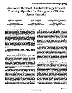
Highly Robust Clustering of GPS Driver Data for Energy Efficient Driving Style Modelling ∗ Michael Breuß and Laurent Hoeltgen and Ali Sharifi Boroujerdi and Ashkan Mansouri Yarahmadi 11th October 2016

Abstract This paper presents a novel approach to distinguish driving styles with respect to their energy efficiency. A distinct property of our method is that it relies exclusively on Global Positioning System (GPS) logs of drivers. This setting is highly relevant in practice as these data can easily be acquired. Relying on positional data alone means that all derived features will be correlated, so we strive to find a single quantity that allows us to perform the driving style analysis. To this end we consider a robust variation of the so called jerk of a movement. We show that our feature choice outperforms other more commonly used jerk-based formulations and we discuss the handling of noisy, inconsistent, and incomplete data as this is a notorious problem when dealing with real-world GPS logs. Our solving strategy relies on an agglomerative hierarchical clustering combined with an L-term heuristic to determine the relevant number of clusters. It can easily be implemented and performs fast, even on very large, real-world data sets. Experiments show that our approach is robust against noise and able to discern different driving styles.

1

Introduction

The driving style has a significant impact on the fuel consumption of a car. Intelligent hybrid cars could adapt to the driving style of the conductor to maximise their mileage. These optimisations could be manifold and range from an efficient assistance of the electric engine to suggestions on energy-optimal routes [6, 11]. In this work we aim to provide a significant step towards integrating the driving style as an additional constraint ∗ The authors thankfully acknowledge the financial support of this work by the German Federal Ministry of Education and Research under grant no. 05M13ICC (RESY).

1

into this objective. We analyse driving behaviour with respect to energy efficiency and provide an automated way to classify it. To allow a broad applicability of our methods, we rely on data that can easily be obtained in any vehicle, as e.g. Global Positioning System (GPS) data logs. Such setups are also attractive due to their relatively low cost and the already abundant availability of GPS enabled devices. However, these benefits are at a certain price. Insufficient accuracy yields noisy samples. Hardware failures may result in a partial or total loss of the data. Furthermore, classifying the driving style without environmental information is a quite challenging task. Driving at a constant 120 km h−1 on a large motorway over lowland is surely an energy efficient way to travel but this may be doubtful when the motorway goes over rolling hills. Traffic jams on motor ways lead to stop and go traffic, which is visible in the logs by frequent small variations in the acceleration and velocity, strongly resembling noise. However, the exact cause of such variations cannot always be deduced with absolute certainty. The driver may as well be looking for a free spot for parking, or his car may simply have broken down. An accurate and robust model must be able to handle these difficulties. Fortunately, notable advances in modelling and understanding driver behaviour have been made in recent years, yet mainly for use in the area of traffic safety engineering. We refer to [10, 12, 13, 14, 15] among the vast amount of literature in that highly active field of research. Although the objective in that field is completely different than in our case, let us still review some works in more detail as we can identify at a technical level some methods related to our approach. In [10, 15] the authors suggest the usage of sensors and simulators to identify driver movements and to predict their behaviour in the forthcoming seconds. These predictions can for example be used to prevent collisions. Both works take a probabilistic approach by analysing dynamic and hidden Markov models. The findings presented in [4, 14] classify drivers according to their imminent risk on the traffic. This classification is obtained by comparing characteristic features of a given driver to information gathered from other vehicles in the vicinity. While the authors of [4] use statistical measures, the authors of [14] combine a clustering algorithm with complex neuroscale and Bayesian factor analyses. A similar research is also performed in [16], where cars are analysed for potentially dangerous behaviour. However, the focus of the latter work lies more on the communication protocols between the traffic participants and not on their classification. All these approaches have in common that they collect significant amounts of data from a heterogeneous pool of sources and that they are designed to analyse the conductor during driving. Many works in the past have also tried to model the conductor himself by analysing his reactions in various settings, see [7, 8]. The authors of the latter work use a car with specialised sensors to measure various information on the drivers. These include position and velocity of the car as well as operation patterns of the gas and brake pedal. The analysis is performed by means of Gaussian mixture and optimal velocity models. In contrast to the first cited references these latter works process the data only after collecting it. Let us now turn to the use of GPS data. Modern potent tracking devices such as navigation systems, cell phones or smartwatches offer huge amounts of information that may be processed to distinguish driving styles. Surprisingly, only few works consider this much simpler approach to restrict the study exclusively on positional 2

information provided by the tracking devices. In [5] the authors seek reckless taxi drivers by analysing the velocity of their cabs and the regions that they pass. The authors of [20] have similar goals but limit themselves to analyse the routes taken. Here, a taxi driver becomes suspicious when his route deviates strongly from those taken by the majority of his colleagues. Let us remark that none of these scenarios require real-time processing capabilities. The information can be stored inside a database first and processed afterwards. In these settings missing additional environmental data can, to a certain extent, be compensated by increasing the amount of positional information. Furthermore, an offline processing of the data allows to use more powerful hardware than available inside a car. Our contribution To our best knowledge we propose in this work for the first time in the literature a method for the analysis of energy efficient driving styles at hand of GPS data collected by drivers. To this end we combine the two different setups presented in the previous paragraphs. Similarly as in the former references, we discern different driving styles, but we focus in doing this on the energy efficiency. Then, our computational approach resembles more the approaches taken in the latter references. Our analysis is based on a set of GPS logs collected beforehand during driving. The processing of the data is done in an offline post-processing step. Thus, one of our contributions is to carry over some ideas from traffic safety engineering and related areas to a novel field of application. Furthermore, we propose some dedicated techniques in order to meet the requirements of our setting and provide a reliable solution in discerning energy efficient driving styles. Our ultimate goal is to classify the drivers solely based on positional information as this is a relevant setting for potential industrial applications of our approach. Let us stress that the use of GPS logs alone is therefore an important issue, and this also distinguishes our work from others that mark the current state-of-the-art in the technically related above-mentioned literature. Despite a high amount of noise in the existing real-world data set [19] that we employ for demonstrating our method we still obtain robust results. Our clustering algorithm employs an improved formulation of the jerk quantity introduced in [9] and used there for driver’s behavioural analysis for traffic safety purposes. Let us also stress that the sole use of positional information implies that it does not make much sense to employ a variety of features based on these data as these will all be naturally correlated. Having just the GPS data at hand it is thus of primal interest to identify one reliable and robust feature to work with. Moreover, this feature should be meaningful by relating to the energy efficiency of driving styles. It is exactly one of our contributions to provide this by means of a novel jerk-based feature. In combination with an agglomerative hierarchical clustering algorithm we achieve a reliable classification result with reasonable computational effort. Furthermore, we suggest a simple strategy to determine a reasonable amount of clusters. Experimental results show that our approach is more robust than a straight forward adaptation of previous approaches. In the paper we proceed as follows. First we give a detailed physical-based argumentation that motivates the use of the jerk as a meaningful feature for our application.

3

This is followed by a presentation of our clustering method for classifying drivers. In the final section we discuss at hand of the application of our method at the real-world data set [19] the viability of our approach. The paper is finished by a summary and conclusion.

2

Motivation: On energy efficiency and jerk

Let us now motivate our use of the jerk as the underlying feature of our investigation. Thereby we comment on two important aspects in pattern recognition, physical significance of the feature and useful invariances for our application.

2.1

Basic physical considerations

For modelling we consider the movement of a car during a fixed time frame which we parametrise via the time t ∈ [0, T ]. For simplicity of notation, we assume that the car performs a 1-D movement along a straight horizontal path S in this time frame. We denote by s0 and sT the starting point and the end point of S, respectively, and we write d for the length of the path. Concerning the time-dependent position of the car along S, we make use of a corresponding function x(t). We sometimes denote by v = x˙ := x(t) ˙ = v(t) the velocity and by a = x¨ = v˙ the acceleration of the car. We assume for simplicity that the mass mc of the car is a constant over the considered time frame (neglecting e.g. mass loss due to consumed fuel). Another fundamental yet not too obvious assumption for our modelling is that the driver aims to travel the distance d of path S during the considered time frame over the time interval [0, T ]. This underlying assumption is required as otherwise one may realise a fuel saving driving style by performing a full break and shutting off the car. Let us note that this underlying assumption is in accordance to the content of given data after our preprocessing as GPS logs of cars standing still will be discarded. Let us now assert that in the engine, fuel is transformed into mechanical work W . In order to obtain a measure for fuel consumption (denoted by fc), the transformation process has to be related to consumption over the considered time frame, or equivalently to the distance d passed during the time frame. To this end we opt to measure fc via the generated mechanical work over distance d and assume the proportionality law: fc ∼

W d

or

fc = p

W d

(1)

where the proportionality constant p is given by the combustion efficiency of the engine. Let us note that in terms of physical measurement units, we have by [d] = m   W [fc] = = kg m/s2 = N (2) d that means the fuel consumption is proportional to the force F with [F] = N needed to move the car along S.

4

By considering now Newton’s second law we have for the 1-D movement of the car: W = F ·d

W = F = mc · a¯ d

⇔

(3)

where a¯ is the acceleration needed over [0, T ] in order to move the car from s0 to sT over distance d along S. As a consequence of (1) to (3), we obtain fc ∼ a¯

or

fc = p · mc · a¯

(4)

Let us now consider the situation that the car enters S with a certain velocity v¯ > 0. Then by basic physical principles the kinetic energy E = 12 mv¯2 corresponds to the work W stored in the movement. In an ideal, frictionless environment the car moves on with constant speed v, ¯ and there is no need to install an additional acceleration to hold v¯ as would be desired by a driver in order to travel along S during the considered time frame. It is clear that in reality where e.g. friction takes place, a certain acceleration is needed to allow the driver to travel the distance d along S during [0, T ]. Since fc ∼ a¯ this also means that a certain amount of fuel has to be used up. The question arises how such an acceleration should be applied over [0, T ] in the most fuel saving manner. One may imagine here e.g. that it could be beneficial to accelerate very strongly at the beginning over [0, ε], 0 < ε  1, and letting the car roll over the remaining time frame [ε, T ] to arrive then at time T at point sT . Let us note in this context that the acceleration a¯ just gives a total value over [0, T ] and does not reveal how this total value has to be realised. In order to identify the most fuel saving way to accelerate, it is obvious by fc ∼ a¯ that we have to minimise the total required acceleration a. ¯ To this end we now consider the main forces acting on the car. We propose to constitute as main sources of fuel consumption frictional forces and aerodynamic resistance. Since forces are acting (by fundamental physical principles) in an additive and independent way on the car, it will turn out that we may discuss them separately. Before doing that, we first have another look at the basic mechanism behind fuel consumption itself. We consider again (1) and formulate the fuel consumption using the total transformed fuel over the considered time frame. For the computation we make explicit by taking the absolute of W , that braking does not generate fuel: fc ∼

Z T 0

|W (t)| dt

W =F·d

∼

Z T 0

|a(t)| dt =

Z T

|x(t)| ¨ dt

(5)

0

To minimise fuel consumption during the transformation process to mechanical work, it is therefore optimal to uphold a constant velocity since the minimiser of the above expression is obtained for (x¨ = 0) ⇔ (v = constant). Let us turn to frictional forces Ff riction = η · Fn , where η is the friction coefficient and Fn = mc g the normal force described by the constant mass of the car mc and the gravitational constant g. In this context let us note that we impose indirectly that the car moves approximately horizontally. Assuming that η is constant over our time frame, this means that to negate frictional forces implies to uphold a constant acceleration a, compare (3). 5

Turning to the aerodynamic resistance of a car, this may be modelled by a force Fair ∼ v2 = x˙2 . In order to minimise the required acceleration negating aerodynamic resistance, we thus have to find the minimiser of Z T

min x

(x(t)) ˙ 2 dt

(6)

0

subject to boundary conditions x(0) = s0 and x(T ) = sT . The corresponding optimality condition reads as 2v˙ = 0. Therefore it is optimal w.r.t. fuel consumption to uphold a constant velocity in order to negate the aerodynamic resistance. This can be realised by a constant acceleration added to the one we found to be required to negate frictional forces. As a consequence of our investigation, it is optimal to negate the fuel-consuming forces by a constant acceleration, thereby upholding a constant velocity of the car. Since a constant acceleration implies a˙ = 0, one may detect instances of potential fuel-wasting driving by evaluating a˙ = v, ¨ and it appears to be an energy-efficient driving style if |v| ¨ is kept low by a driver. This result is in accordance with the intuition that drivers aiming at an energy saving driving style usually perform smooth accelerations and braking, whereas racy, highly energy consuming drivers tend to have a more abrupt driving style. Also dense urban traffic with the typical changes in acceleration and deceleration which is notorious for leading a high fuel consumption is represented by strong instances of |v|. ¨

2.2

Invariances

As discussed, the quantity v¨ = a˙ describes the variation of the acceleration of a car. However, the positional GPS data gathered in our database also allows us to formulate quantities that offer certain invariances. Our analysis should not depend on an absolute positioning and yield the same findings whether we analyse cars in Europe or in Asia. Such an invariance can be introduced by taking derivatives of the movement. The velocity is independent of the exact location of a car. Further, the acceleration of a car driving smoothly with 130 km h−1 is similar to a car driving with 50 km h−1 . If the environmental circumstances are adequate, then both drivers should have the same classification. This observation motivates the usage of a feature with a sufficient large set of invariances. The quantity v¨ is invariant under affine transformations of the velocity and offers these benefits, too.

2.3

Formalisation

We conclude our motivation by observing that the quantity v¨ is well-known in physics as jerk. For convenience, we formalise this observation at hand of the following definition. Definition 1 (Jerk function). The jerk j(t) describes the third order derivative of the 3 position x(t) with respect to time: j(t) := dtd 3 x (t). Let us note that we refer here to jerk in terms of the derivative of a position x since our input data is given by positions. 6

Figure 1: Velocity, acceleration and jerk patterns corresponding to a calm and a racy driver in contrast to the same quantities of a movement pattern containing noisy GPS logs. Note that the y-axis in each plot has a completely different range. Either of the acceleration or jerk pattern could distinguish the calm from the aggressive driver, efficiently. In case of the noisy movement pattern, still either of the acceleration or jerk pattern could efficiently reveal the existence of a noisy GPS log. Our proposed exponential based feature ω, cf. (7), shows high robustness w.r.t. noise. It helps to accommodate noisy movement patterns totally in a separate cluster. We also remark that in [9], the authors use already the jerk function to classify drivers with respect to their aggressiveness, however, as we have shown, the jerk is also a reasonable physical quantity related to energy consumption during driving.

3

Driving style analysis by GPS data

Relying exclusively on GPS data, as provided by navigation systems and tracking devices, comes with a certain number of hurdles that need to be overcome. Our goal is to classify drivers with respect to their driving style. Currently, this analysis is done offline. We first collect the data and store it in a database. The processing and classification is done afterwards. To this end we measure the drivers’ spatio-temporal positions. Definition 2 below gives us a formal framework to work in. Positional data of the cars comes in form of coordinate pairs (xi , yi ) ∈ R2 . Each pair is accompanied with a label containing the time stamp ti when the position has been recorded. This set of discrete samples gives us a complete description of the movement of a car in space and time. Yet, our focus lies on the analysis of moving cars. Therefore, we use a more specific structure to represent the displacement of a vehicle. Definition 2 (Time frame, Movement pattern). We define a time frame of size ` a sorted vector T ∈ R` containing ` individual time stamps in non-decreasing order. We call movement pattern of size ` a pair {T, P} consisting of a time frame T of size ` with the corresponding positional data P := {(xi , yi ) | i = 1, . . . , `} if the car is not standing still during any moment within the complete time frame. 7

Thus, we speak of a movement pattern if the car does not stop during a considered time interval. We elaborate a method to discard the idling objects from our data set in the next section.

3.1

Data preprocessing

In order to apply our method we need to preprocess the given data set of GPS logs. First of all, we discard corrupted or meaningless data. After the preprocessing our data should only consist of movement patterns as defined in Definition 2. To this end we remove all logs for which the following conditions hold: 1. All GPS logs having the same longitude and latitude values as well as the same sampled time as their adjacent logs. These logs represent repeated GPS values being sampled at least twice due to hardware failure. 2. All GPS logs with same longitude and latitude having different sampled time compared to their adjacent GPS logs. These GPS logs represent a car standing still. The preprocessing is necessary to ensure reasonable findings. However, it also introduces holes in the displacement history of the analysed car. Certain records are contiguous over long time intervals whereas others might only run for a few seconds before a gap occurs. Our forthcoming analysis is based on statistical measures of the movement pattern. To allow a meaningful and unbiased comparison we additionally drop movement patterns that are too short and break down those that are too long into several smaller ones. In this work we discard all movements patterns with less than 10 samples and split them if they exceed a length of 24. After the preprocessing we obtain about 3225 movement patterns from the real-world data set [19].

3.2

Clustering movement patterns by a novel jerk based feature

Let us implement our underlying considerations about the jerk in the context of a typical example of GPS data. As discussed, important physical quantities in the description of the behaviour of drivers are the position, velocity, and acceleration of their car. Figure 1 depicts an example of velocity, acceleration, and jerk obtained from a movement pattern of a calm driver, a racy driver, along with a movement pattern containing a noisy log. Even though a distinction among the three shown patterns could be deduced from the velocity and acceleration alone, the jerk has the benefit of magnifying big abrupt changes in the acceleration much more than smaller ones and therefore, simplifies the noise detection significantly. This can clearly be observed in the noisy movement pattern shown in Fig. 1. The previous arguments together with our physical considerations constitute the principal motivations to use the jerk as starting point in our work. Our exponential based feature proposed in (7) takes advantage of the elaborated properties. The authors of [9] use the ratio between the standard deviation of the jerk function and its mean value as feature to distinguish between calm, normal and aggressive drivers. Their method uses a data set obtained from [1]. The movement patterns are augmented with additional information that indicates the road type (e.g. freeway, ramps, local roads, 8

1

Feature value

0.8

Proposed method by [9] ω Mean Standard deviation

0.6 0.4 0.2 0 −0.2

0

500

1000 1500 2000 Number of movement patterns

2500

3000

Figure 2: The sorted values of mean, standard deviation, the feature proposed by [9] and our proposed feature for all preprocessed movement patterns from [19]. The approach from [9] only yields two distinct classes and cannot detect noise. On the other hand, the curve representing the mean is almost flat, rendering it very difficult to distinguish different clusters. The standard deviation depicts a similar behaviour as our proposed feature but bears a less stable behaviour towards the end. Our feature yields a curve with a clear monotonic increase and a notable elbow at the end. Thus, we obtain the same segregation ability as the standard deviation but also a clearer threshold for the noise detection, which is given by the samples located in the elbow. etc.) as well as the mean jerk value expected for the corresponding road type. This information is usually not available in standard GPS logs. Furthermore, the classification from [9] uses a hard threshold. We believe, that a soft thresholding is better suited for classifying such complex patterns as driving styles. To tackle the just mentioned problems we propose a few adaptions in the forthcoming paragraphs. Modelling details Our proposed method seeks to classify driving style using an alternative formulation which also considers the jerk. We suggest to use a clustering strategy exclusively based on the following feature:   1  ω ({T, P}) := exp − q (7)
σ j{T,P} Here, j{T,P} is the array of jerk values for each position in the movement pattern {T, P}. These are computed by means of standard finite difference schemes. The function σ denotes the standard deviation. The motivation for proposing this feature is as follows. The exponential part of (7) discriminates those movement patterns having a very high amount of fluctuation rate around their mean jerk values. They occur due to the existence of at least one noisy GPS log inside the movement pattern or a dubious driving style with a large number of strong accelerations and decelerations. Further, in order to discern drivers with lower jerk fluctuation rates we consider the square root of the standard deviation inside the exponential function. This facilitates the formation of a smooth elbow in our proposed feature ω, see Fig. 2. 9

Algorithm 1: Agglomerative hierarchical clustering of movement patterns Data: A set of movement patterns. Result: A clustering of the input movement patterns. 1 Compute the feature value ω from (7) for each movement pattern. 2 Place each feature value in its own cluster. 3 repeat 4 Find pair of clusters that minimises (8). 5 Merge this pair into a single cluster. 6 until a single cluster is left 7 return the smallest number of clusters, that yielded a decrease in (9) below a threshold T .

In our experiments, the modified jerk feature yielded the most intuitive and reliable clustering results. Small feature values correspond to those movement patterns representing drivers with less accelerations and decelerations in their driving patterns. An energy-saving driving style can therefore be identified by small feature values, whereas more racy drivers will usually exhibit larger feature values. Algorithmic details Two classic and well studied approaches to classify data are partitional and hierarchical clustering methods. The latter have the advantage to yield a complete scale evolution for all possible numbers of clusters. Since the optimal number of clusters is hard to predict, we opt for such a flexible approach using an agglomerative clustering method. Such a method starts by taking singleton clusters at the bottom level and continues merging two clusters at a time to build a bottom-up hierarchy of clusters. We employ Ward’s criterion for the merging strategy [17, 18]. It makes use of the standard k-means squared error (SSE) to determine the distance between two clusters. For any two clusters, Ca and Cb , Ward’s criterion is calculated by measuring the increase in the value of the SSE for the clustering obtained by merging them into a single cluster Ca ∪Cb . The characteristic number of Ward’s criterion is defined as follows:
2 |Ca | |Cb | ` k caν − cbη ∑ ∑ |Ca | + |Cb | ν=1 η=1

(8)

where the cluster Cx has the individual components cxν . The cardinality of a cluster is denoted by |Cx |. We iteratively merge clusters in a bottom-up fashion. At the bottom level, each computed feature point is considered. Then, at each new level we merge the pair of clusters that minimises (8). The algorithmic details of the agglomerative hierarchical clustering are also given in Algorithm 1. The optimal number of clusters is obtained through an L-curve heuristic [2, 3]. We compare the number of clusters against the within-cluster sum of squares (WCSS) and consider the smallest number of clusters that yields a decrease in the WCSS below a

10

2

1

Clusters

1

Clusters

Clusters

1

2

3

-1

-0.5

0

0.5

1

5

-1

-0.5

Silhouette Values

(a) Here the number of clusters is considered to be three. In this case a group of drivers in the 2nd cluster is probably not optimally labelled. It is not possible to decide if they belong to average fuel consuming drivers or to noisy patterns. Only the energy saving drivers could be clearly located in the 1st cluster.

3

4

4

3

2

0

0.5

1

Silhouette Values

(b) A minimal number of drivers with a negative silhouette index is found with 4 clusters. This clustering seems to be the best labelling. Noisy driver patterns are likely to be found in the 4th cluster. All energy saving drivers are located in the 1st cluster and average fuel consuming drivers expand across two classes in the 2nd and 3rd cluster, respectively.

-1

-0.5

0

0.5

1

Silhouette Values

(c) By increasing the number of clusters to five, drivers with negative silhouette indices appear even in the 1st cluster with small ω values. This depicts a clustering result which may not be considered as optimal, since almost all clusters accommodate dissimilar drivers inside them.

Figure 3: The silhouette indices of a clustering setup establishing (a) three, (b) four and (c) five distinct groups of ω values of the central area drivers in Beijing. Inside each cluster, the more positive a silhouette index of a feature, the more similar is the feature to its group-mates which indicates a good clustering. given threshold. The WCSS is given by: M

∑ ∑ kx − ca k22

(9)

a=1 x∈Ca

where M is the total number of clusters and ca is the centroid of cluster Ca . In our WCSS based experiments the optimal number of clusters was usually found to be four. In what follows, the silhouette index SIi (10) is computed for members of each four established clusters: SIi =

bi − ai max(ai , bi )

(10)

Here, ai is the mean distance between any cluster member ωi to all other members in same cluster and bi is the mean distance among the cluster member ωi and all other members in next nearest cluster. The computed SIi corresponding to ωi takes negative or positive values in range of [−1, +1] as being mostly dissimilar or similar to other members in same cluster. Well established clusters require silhouette indices to be positive over their members. Our best clustering result is analysed with respect to its labelling in Fig. 3 (b). The negative silhouette indices inside the 4th cluster represent the compactly accommodated 11

noisy ω values. This observation validates our approach for identifying the noisy values. In addition, only a few members in the 2nd cluster are wrongly located making the final clustering result meaningful. Let us emphasise that an alternative strategy would also be possible with the kmeans algorithm. However, k-means needs to be restarted for each new amount of clusters and thus adds a significant computational burden if the number of clusters is not predetermined exactly.

4

Experimental results and validation

In order to investigate the efficiency of our proposed feature we consider a database with GPS logs from two distinct parts of Beijing city [19]. The whole database contains the trajectories of more than 10,000 taxis collected during the period of Feb. 2 to Feb. 8, 2008. In total there are more than 17 million GPS logs that cover a total distance of around 9 million kilometres. Since the data set corresponds to various taxi drivers we expect to find many different driving styles in this data set. The regions that we consider contain a vast area of Beijing city centre and a freeway expanded from east to west. We preprocess the logs as described in Section 3.1 and obtain correspondingly 3225 patterns for the city centre and 106 movement patterns for the freeway. All our feature values are computed according to (7). In a first experiment we compare the Beijing city centre feature values as by (7) to other commonly used feature choices. The findings are visualised in Fig. 2. We compare our suggested feature against the mean value and standard deviation as well as the jerk-based feature from [9]. The approach from [9] (proposed for the purpose of analysing driver behaviour, not for energy efficiency) yields a clear cut. It segregates our drivers into two categories, namely defensive and aggressive drivers as by the context of the work [9]. For this classification we used the parameter suggestions from [9]. We selected a window size of 10 seconds and set the parameters normthreshold and aggthreshold to 0.5 and 1 respectively. This method yields a very clear threshold that discerns the two classes of drivers. However, it is unable to detect noisy data. If we consider the average value and standard deviation as features then we are able to detect the corrupted data but a discrimination of the remaining drivers becomes difficult. All their feature values are very close to each other. Finally, our proposed feature yields a larger range of values as well as a clear jump at the end of the curve. Thus, we are in the position to distinguish different driving styles as well as filtering out noisy patterns. Next, we evaluate our proposed approach by applying the agglomerative clustering detailed in Algorithm 1. The distribution of all feature values among the different clusters is visualised in Fig. 4. As we can see, the feature values from the first cluster and the fourth cluster are clearly different from those in the second and third cluster. It confirms our expectations. The first cluster contains the energy saving drivers, whereas cluster 4 is supposed to contain noise as well as the highly fuel consuming drivers. Finally, the majority of the drivers lies within the bounds of the second and third cluster and present an average fuel consumption.

12

0.7 0.6

Freeway Central Area

Feature values ω

0.5 0.4 0.3 0.2 0.1 0.0

Cluster 1

Cluster 2

Cluster 3

Cluster 4

Figure 4: A whisker plot showing the distribution of the feature values among the different clusters for our two experimental setups. The box marks the boundaries of the first and third quartiles, while the bars indicate the full extent of the feature values in that cluster. The horizontal line indicates the median. As we can see, the first cluster and on the other hand the second and third cluster are well separated in terms of feature values. There is a continuous overlap from the second to the third cluster. These two clusters represent the majority of the drivers with an average fuel consuming driving style, with tendency towards being more (cluster 2) and less (cluster 3) energy efficient. The first cluster represents the energy saving drivers and the last cluster the drivers with a high fuel consumption, containing also noisy driver patterns.

13

Findings for Beijing city centre area The clusters 1, 2, and 3 are totally noise free and could be adopted as an accurate driver’s behavioural model. The within-cluster sum of squares (WCSS) index does not show any remarkable amount of reduction by adding a 5th cluster or more. Hence, according to our L-term heuristic, we should set the final number of clusters to 4. The noisy patterns are located fully in cluster number 4. Let us stress that our algorithmic proceeding that results in setting the number of clusters to four is confirmed in an independent way by evaluating the silhouette indices as shown in Fig. 3. This is shown here exemplarily for the data of the Beijing city centre area but also holds for the other analysed data. Findings for the freeway area The clusters 1 resp. 2 are noise free. The L-term strategy suggests to use 4 clusters in this case. Since we only have very few feature values in this area our algorithm does not yield a cluster solely containing noise. However, the 4th cluster contains partially the noisy movement patterns. Such a cluster was present for the Beijing centre area, where the 4th cluster was filled with corrupted patterns only. This observation also shows that our classification algorithm benefits from having an extremely large amount of samples to its avail. This is a realistic scenario in an industrial application where large amounts of data can be collected e.g. via navigation systems. The more samples we can process the clearer we can distinguish noise and classify the individual drivers.

5

Summary and conclusion

In this paper we have shown that it is possible to discern different driving style patterns with respect to their energy consumption from their GPS logs alone. To this end we use a dedicated variation of the jerk feature and combine it with a hierarchical clustering approach. Our model is quite simple but still capable of discriminating drivers into different classes and filtering out noisy data logs. Let us note again that the use of just the GPS logs is highly relevant for a potential industrial use of our results in the context of navigation systems. In the future we aim to combine the driver model information with other optimisation tools mentioned in the introduction in order to improve the energy efficiency of hybrid cars.

References [1] Argonne National Laboratory. http://www.transportation.anl.gov/ modeling_simulation/PSAT/index.html. Last access: 27/05/2015. [2] P. C. Hansen. Analysis of discrete ill-posed problems by means of the L-curve. SIAM Review, 34(4):561–580, 1992.

14

[3] Per Christian Hansen and Dianne Prost O’Leary. The use of the l-curve in the regularization of discrete ill-posed problems. SIAM Journal on Scientific Computing, 14:1487–1503, 1993. [4] T. Imamura, H. Yamashita, MD bin R. Othman, Z. Zhang, and T. Miyake. Driving behavior classification river sensing based on vehicle steering wheel operations. In Proceedings of the SICE Annual Conference, pages 2714–2718, 2005. [5] Z. Liao, Y. Yu, and B. Chen. Anomaly detection in GPS data based on visual analytics. In Proceedings of the IEEE Symposium on Visual Analytics and Science Technology, pages 51–58, 2010. [6] S¨oren Merting, Christian Schwan, and Martin Strehler. Routing of Electric Vehicles: Constrained Shortest Path Problems with Resource Recovering Nodes. In 15th Workshop on Algorithmic Approaches for Transportation Modelling, Optimization, and Systems, volume 48, pages 29–41, 2015. [7] JohnA. Michon. A critical view of driver behavior models: What do we know, what should we do? In Human Behavior and Traffic Safety, pages 485–524. Springer US, 1985. [8] C. Miyajima, Y. Nishiwaki, K. Ozawa, T. Wakita, K. Itou, K. Takeda, and F. Itakura. Driver modeling based on driving behavior and its evaluation in driver identification. Proceedings of the IEEE,, Vol. 95,:pp. 427–437, 2007. [9] Y. L. Murphey, R. Milton, and L. Kiliaris. Driver’s style classification using jerk analysis. In IEEE Workshop on Computational Intelligence in Vehicles and Vehicular Systems, pages 23–28, 2009. [10] A. Pentland and A. Liu. Modeling and prediction of human behaviour. Neural Computation, 11:229–242, 1999. [11] S. Pickenhain and A. Burtchen. Optimal energy control of hybrid vehicles. In Proceedings of 6th International Conference on High Performance Scientific Computing, 2015. accepted for publication. [12] M. C. G. Quintero, J. O. Lopez, and A. C. C. Pinilla. Driver behavior classification model based on an intelligent driving diagnosis system. In Proceedings of the 15th International IEEE Conference Intelligent Transportation Systems, pages 894–899, 2012. [13] M.C. G. Quintero, J. A. O. L´opez, and J. M. P. R´ua. Intelligent erratic driving diagnosis based on artificial neural networks. In Proceedings of the IEEE ANDESCON Conference, pages 1–6, 2010. [14] M. Rigolli, Q. Williams, M. J. Gooding, and M. Brady. Driver behavioural classification from trajectory data. In Proceedings of the International IEEE Conference on Intelligent Transportation Systems, volume 6, pages 889–894, 2005.

15

[15] A. Sathyanarayana, P. Boyraz, and J. H. L. Hansen. Driver behavior analysis and route recognition by hidden markov models. In Proceedings of the IEEE International Conference on Vehicular Electronics and Safety, pages 276–281, 2008. [16] V. Verroios, C. M. Vicente, and A. Delis. Alerting for vehicles demonstrating hazardous driving behavior. In Proceedings of the 11th ACM International Workshop on Data Engineering for Wireless and Mobile Access, pages 894–899, 2012. [17] J. Ward. Hierarchical grouping to optimize an objective function. Journal of the American Statistical Association, 58(301):236–244, 1963. [18] D. Wishart. An algorithm for hierarchical classifications. Biometrics, 25(1):165– 170, 1969. [19] Jing Yuan, Yu Zheng, Chengyang Zhang, Wenlei Xie, Xing Xie, and Yan Huang. T-drive: Driving directions based on taxi trajectories. In ACM SIGSPATIAL GIS 2010, pages 99–108, 2010. [20] Daqing Zhang, Nan Li, Zhi-Hua Zhou, Chao Chen, Lin Sun, and Shijian Li. ibat: Detecting anomalous taxi trajectories from gps traces. In Proceedings of the 13th International Conference on Ubiquitous Computing, pages 99–108. ACM, 2011.

16