problem as “appearance-only SLAM” because our aim is not limited to
localization. ... incrementally constructs a map, and so is effectively a SLAM
technique.
1
Highly Scalable Appearance-Only SLAM – FAB-MAP 2.0 Mark Cummins and Paul Newman, Oxford University Mobile Robotics Group
Abstract—We describe a new formulation of appearance-only SLAM suitable for very large scale navigation. The system navigates in the space of appearance, assigning each new observation to either a new or previously visited location, without reference to metric position. The system is demonstrated performing reliable online appearance mapping and loop closure detection over a 1,000 km trajectory, with mean filter update times of 14 ms. The 1,000 km experiment is more than an order of magnitude larger than any previously reported result. The scalability of the system is achieved by defining a sparse approximation to the FAB-MAP model suitable for implementation using an inverted index. Our formulation of the problem is fully probabilistic and naturally incorporates robustness against perceptual aliasing. The 1,000 km data set comprising almost a terabyte of omni-directional and stereo imagery is available for use, and we hope that it will serve as a benchmark for future systems.
I. I NTRODUCTION This paper is concerned with the problem of appearancebased place recognition at very large scale. We refer to the problem as “appearance-only SLAM” because our aim is not limited to localization. New observations can be determined to originate from previously unseen locations. Thus the system incrementally constructs a map, and so is effectively a SLAM technique. However, instead of estimating the positions of landmarks in metric coordinates, the system estimates their positions in an appearance space. Because distinctive places can be recognised even after unknown vehicle motion, appearanceonly SLAM techniques provide a natural solution to the problems of loop-closure detection, multi-session mapping and kidnapped robot problems. The approach is thus complementary to metric SLAM methods that are typically challenged by these scenarios. We have addressed these issues previously in [1], [2]. This paper advances the state of the art by describing a new formulation of the approach which extends the applicable scale of the techniques by at least two orders of magnitude. We validate the work on a 1,000 km data set; the largest experiment conducted with systems of this kind by a considerable margin. The data set, including omni-directional imagery, 20Hz stereo imagery and 5Hz GPS, is available for use by other researchers and is intended to serve as a benchmark for future systems. II. R ELATED W ORK The foundations of appearance-based navigation have a long history within robotics, however there have been a number of impressive technical advances quite recently. For example, in the largest appearance-based navigation experiment we are aware of [3], a set of biologically inspired approaches is employed. The system achieved successful loop closure detection
Figure 1: Segments of the 1,000km evaluation trajectory (showing ground truth positions). and mapping in a collection of more than 12,000 images from a 66 km trajectory, with processing time of less than 100 ms per image. The appearance-recognition component of the system is based on direct template matching, so scales linearly with the size of the environment. Operating at a similar scale, Bosse and Zlot describe a place recognition system based on distinctive keypoints extracted from 2D lidar data [4], and demonstrate good precision-recall performance over an 18 km suburban data set. Related results, though based on a less scalable correlation-based submap matching method, were also described in [5]. Olson described an approach to increasing the robustness of general loop closure detection systems by using both appearance and relative metric information to select a single consistent set of loop closures from a larger number of candidates [6]. The method was evaluated over several kilometers of urban data and shown to recover high-precision loop closures even with the use of artificially poor image features. Other appearance-based navigation methods we are aware of have generally been applied only at a more modest scale. Many systems have now been demonstrated operating at scales around a kilometer [7], [8], [9], [10]. Indeed, place recognition systems very similar in character to the one described here have become an important component even of single-camera SLAM systems designed for small-scale applications [11]. Considerable relevant work also exists on the more restricted problem of global localization. For example, Schindler et al. describe a city-scale location recognition system [12] based on the vocabulary tree approach of [13]. The system was demonstrated on a 30,000 image data set from 20 km of
2
urban streets, with retrieval times below 200 ms. Also of direct relevance is the research on content-based image retrieval systems in the computer vision community, where systems have been described that deal with more than a million images [14], [15], [13] . However, the problem of retrieval from a fixed index is considerably easier than the full loop-closure problem, because it is possible to tune the system directly on the images to be recognised, and the difficult issue of new place detection does not arise. We believe the results presented in this paper represent the largest scale system that fully addresses these issues of incrementality and perceptual aliasing. Figure 2: Graphical model of the system. Locations L independently III. S YSTEM D ESCRIPTION A. Probabilistic Model The probabilistic model employed in this paper builds directly on the scheme outlined in [1]. For completeness, we recap it briefly here. The basic data representation used is the bag-of-words approach developed in the computer vision community [16]. Features are detected in raw sensory data, and these features are then quantized with respect to a vocabulary, yielding visual words. The vocabulary is learned by clustering all feature vectors from a set of training data. The Voronoi regions of the cluster centres then define the set of feature vectors that correspond to a particular visual word. The continuous space of feature vectors is thus mapped into the discrete space of visual words, which enables the use of efficient inference and retrieval techniques. In this paper, the raw sensor data of interest is imagery, processed with the SURF feature detector [17], though in principle the approach is applicable to any sensor or combination of sensors, and we have explored multisensory applications elsewhere [18]. FAB-MAP, our appearance-only SLAM system, defines a probabilistic model over the bag-of-words representation. An observation of� local scene appearance captured at time k is denoted Zk = z1 , . . . , z|v| , where |v| is the number of words in the visual vocabulary. The binary variable zi , which we refer to as an observation component, takes value 1 when the ith word of the vocabulary is present in the observation. Z k is used to denote the set of all observations up to time k. At time k, our map of the environment is a collection of nk discrete and disjoint locations Lk = {L1 , . . . , Lnk }. Each location has an associated appearance model, given by the set � p(e1 = 1|Li ), . . . , p(e|v| = 1|Li ) (1) The variable ei models feature existence, as distinct from zi which models feature observation. A detector model relates existence ei to detection zi . The detector model captures the rate of false positive and false negative word detections, and is specified by � p(zi = 1|ei = 0), false positive probability. D: p(zi = 0|ei = 1), false negative probability. (2) A further salient aspect of the data is that visual words do not occur independently – indeed, word occurrence tends to be highly correlated. For example, words associated with car wheels and car doors are likely to be observed simultaneously.
generate existence variables e. Observed variables zi are conditioned on existence variables ei via the detector model, and on each other via the Chow Liu tree.
We capture these dependencies by learning a tree-structured Bayesian network using the Chow Liu algorithm [19], which yields the optimal approximation to the joint distribution over word occurrence within the space of tree-structured networks. Importantly, tree-structured networks also permit efficient learning and inference even for very large visual vocabulary sizes. The graphical model of the system is shown in Figure 2. Given our probabilistic appearance model, localization and mapping can be cast as a recursive Bayes estimation problem, closely analogous to metric SLAM. A pdf over location given the set of observations up to time k is given by: p(Li |Z k ) =
p(Zk |Li , Z k−1 )p(Li |Z k−1 ) p(Zk |Z k−1 )
(3)
Here p(Li |Z k−1 ) is our prior belief about our location, p(Zk |Li , Z k−1 ) is the observation likelihood, and p(Zk |Z k−1 ) is a normalizing term. We briefly discuss the evaluation of each of these terms below. Full details can be found in [1]. Observation Likelihood: To evaluate the observation likelihood, we assume independence between the current and past observations conditioned on the location, and make use the Chow Liu model of the joint distribution, yielding: p(Zk |Li )=p(zr |Li )
|v| Y
p(zq |zpq , Li )
(4)
q=2
where zr is the root of the Chow Liu tree and zpq is the parent of zq in the tree. Each term in the product can be further expanded as: p(zq |zpq , Li ) =
X
p(zq |eq = seq , zpq )p(eq = seq |Li )
seq ∈{0,1}
(5) which can be evaluated explicitly. Location Prior: The location prior p(Li |Z k−1 ) is obtained by transforming the previous position estimate via a simple motion model. The model assumes that if the vehicle is at location i at time k − 1, it is likely to be at one of the topologically adjacent locations at time k.
3
Normalization: In contrast to a localization system, a SLAM system requires an explicit evaluation of the normalizing term p(Zk |Z k−1 ) , which incorporates the probability that the current observation comes from a previously unknown location. If we divide the world into the set of mapped locations M and the unmapped locations M , then p(Zk |Z k−1 )
=
X
p(Zk |Lm )p(Lm |Z k−1 )
(6)
m∈M
+
X
p(Zk |Lu )p(Lu |Z k−1 )
(7)
u∈M
The second summation cannot be evaluated directly because it involves all possible unknown locations. However, if we have a large set of randomly collected location models Lu , (readily available from previous runs of the robot or other suitable data sources such as, for our application, Google Street View), we can approximate the summation by Monte Carlo sampling. Assuming a uniform prior over the samples, this yields: p(Zk |Z k−1 ) ≈
X
p(Zk |Lm )p(Lm |Z k−1 )
(8)
m∈M
+p(Lnew |Z k−1 )
ns X p(Zk |Lu ) ns u=1
(9)
where ns is the number of samples used, and p(Lnew |Z k−1 ) is our prior probability of being at a new location. Data Association: Once the pdf over locations is computed, a data association decision is made. The observation Zk is used either to initialize a new location, or update the appearance model of an existing location. Each component of the appearance model is updated according to: p(Zk |ei = 1, Lj )p(ei = 1|Lj , Z k−1 ) p(Zk |Lj ) (10) In the case of new locations, the values p(ei = 1|L) are initialized to the marginal probability p(ei = 1) derived from the training data, and then the update is applied. p(ei = 1|Lj , Z k ) =
B. Efficient Large Scale Implementation - FAB-MAP 2.0 The probabilistic model defined above has been used previously in [20], [1], and an approximate inference procedure for it was described in [2]. A key contribution of this paper is to describe a modified version of the model which extends its applicability by more than two orders of magnitude in scale. For a highly scalable system, we turn to an inverted index retrieval architecture. In computational terms, the inverted index approach essentially scales indefinitely [21]. However, FAB-MAP is not directly implementable using an inverted index structure, because the appearance likelihood p(Zk |Li ) Q|v| requires evaluation of Equation 4, q=2 p(zq |zpq , Li ). The computation pattern is illustrated in Figure 3. Every observation component contributes to the appearance likelihood, including negative observations – those where zq = 0, words not detected in the current image. As such, it does not have the sparsity structure that enables inverted index approaches to
scale. Perhaps surprisingly, we have found that simply ignoring the negative observations has a detrimental impact on place recognition performance. Thus we seek a formulation that will enable efficient implementation, but preserve the information inherent in the negative observations. To enable an inverted index implementation, we modify the probabilistic model in two ways. Firstly, we place some restrictions on the probabilities in the location models. Recalling Equation 1, locations models are parametrized as � p(e1 = 1|Lj ), . . . , p(e|v| = 1|Lj ) , that is, by a set of beliefs about the existence of features that give rise to observations of the words in the vocabulary. Let p(ei |Lj )|{0} denote one of these beliefs, where the subscript {0} indicates the history of observations that have been associated with the location. Thus {0} denotes one associated observation with zi = 0, and {0, 0, 1} denotes three associated observations, with zi = 1 in one of those observations. Further, let p(ei |Lj )|0 indicate that in all observations associated with the location, zi =0. In the general probabilistic model described in Section III-A, p(ei |Lj )|0 can take on a range of values - for example, p(ei |Lj )|{0} 6= p(ei |Lj )|{0,0} , as the belief in the non-existence of the feature increases as more supporting observations become available. In FAB-MAP 2.0, the model is restricted so that p(ei |Lj )|0 must take the same value for all locations; it is clamped at the value p(ei |Lj )|{0} . This restriction enables an efficient likelihood calculation, illustrated in Figure 4. Consider the calculation of one component of the observation likelihood, as per Equation 5, across all locations in the map. In the unrestricted model, this will involve a computation for each location, as illustrated in Figure 4(a). In the restricted model, Figure 4(b), the value of the observation likelihood in all locations where p(ei |Lj )|0 is the same. Working with log-likelihoods, and given that the distribution will later be normalized, the calculation can be reorganized so that it has a sparse structure, Figure 4(c), which allows for efficient implementation using an inverted index. We emphasize the fact that this restriction placed on the model is rather slight, and most of the power of the original model is retained. During the exploration phase, when only one observation is associated with each location, the two schemes are identical1 . The restricted terms p(ei |Lj )|0 can (and do) vary with i (word ID), and also with time. Treatment of correlations between words, of perceptual aliasing, and of the detector model remains unaffected. The second change we make to the model concerns data association. Previously, data association was carried out via Equation 10, updating the beliefs p(e|L). Effectively this amounts to capturing the average appearance of a location. For example, if a location has a multi-modal distribution over word occurrence, such as a door that may be either open or shut, then the location appearance model will approach the mean of this distribution. In FAB-MAP 1.0, when computation increased swiftly with the number of appearance models to be evaluated, this was a reasonable design choice. For FAB-MAP 2.0 we switch to representing locations in a sample-based 1 Assuming
the detector model does not change with time.
4
(a) FAB-MAP 1.0
(b) FAB-MAP 1.0 with Bennett Bound
(c) FAB-MAP 2.0
Figure 3: Illustration of the amount of computation performed by the different models. The shaded region of each block represents the appearance likelihood terms p(zq |zpq , Li ) which must be evaluated. In (a), FAB-MAP 1.0 [1], the likelihood must be computed for all words in all locations in the map. Using the Bennett bound approximate inference procedure defined in [2], unlikely locations are discarded during the computation, yielding the evaluation pattern shown in (b). The restrictions imposed in FAB-MAP 2.0 allow a fully sparse evaluation, (c).
Algorithm 1 Log-likelihood update using the inverted index.
(a) Unrestricted Model
(b) Restricted Model
(c) Sparse likelihood update in the restricted model.
Figure 4: Illustration of calculation of one term of Equation 5, the observation likelihood, for a map with four locations. In (a), the model is unrestricted, and the observation likelihood can take a different value for each location. In (b), the restricted model, the likelihood in all locations where the currently considered word was not previously observed is constrained to take the same value. The calculation can now be organized so that it has a sparse structure, (c).
fashion, which better handles these multi-modal appearance effects. Locations now consist of a set of appearance models as defined in Equation 1, with each new observation associated with the location defining a new such model. This change is necessary because of the restrictions placed on word existence probabilities, but is also largely beneficial. While it means that inference time now increases with every observation collected, the system is sufficiently scalable that this is not of immediate relevance, and the greater ability to deal with variable location appearance is preferred. Algorithm 1 gives pseudo-code for the calculation. The calculation is divided into two parts, A and B. Part A deals with the positive observations, those for which zi = 1, while Part B deals with negative observations for which zi = 0. The complexity of Part B is O(#vocab), whereas Part A depends only on the number of words present in a given observation, which is empirically a small constant largely independent of vocabulary size. The straightforward implementation (combining A and B) is in fact fast enough for use, however it can be improved by a caching scheme which eliminates Part B by pre-computing negative votes at the time when the location is added to the map. The negative votes are then adjusted based
Update, Part A (Positive Observations): for zi in Z, such that zi = 1 do: //Get all locations where word i //was observed locations = inverted_index[zi ] for Lj in locations do: //Update the loglikelihood //of each of these locations p(z |z ,L ) loglikelihood[Lj ] += log( p(z i|z pi,L)j ) |0 i pi Update, Part B (Negative Observations): for zi in Z, such that zi = 0 do: locations = inverted_index[zi ] for Lj in locations do: p(z |z
,L )
loglikelihood[Lj ] += log( p(z i|z pi,L)j ) |0 i pi
on the current observation, but do not need to be recomputed entirely. This yields a scheme where the overall complexity is independent of the size of the vocabulary. C. Geometric Verification While a navigation system based entirely on the bag-ofwords likelihood is possible, we have found in common with others [14] that a geometric post-verification stage, which checks that the matched images satisfy epipolar geometry constraints, considerably improves performance. The impact is particularly noticeable as data set size increases - it is helpful on the 70 km data set but almost essential on the 1,000 km set. We apply the geometric verification to the 100 most likely locations (those which maximize p(Zk |Li , Z k−1 )p(Li |Z k−1 )) and to the 100 most likely samples (the location models used to evaluate the normalizing term p(Zk |Z k−1 )). For each of these locations we check geometric consistency with the current observation using RANSAC. Candidate interest point matches are derived from the bag-of-words assignment already computed. Because our aim is only to verify approximate geometric consistency rather than recover exact pose to pose transformations, we assume that the transformation between poses is a pure rotation about the vertical axis. A single point correspondence then defines a transformation, leading to a very rapid verification stage. We accommodate translation
5
between poses by allowing large inlier regions for point correspondences. We have found this simplified model to be effective for increasing navigation performance, while keeping computation requirements to a minimum. Having recovered a set of inliers using RANSAC we recompute the location’s likelihood by setting zi = 0 for all those visual words not part of the inlier set. A likelihood of zero is assigned to all locations not subject to geometric verification. For the 1,000 km experiment, the maximum time taken to rerank all 200 locations was 145 ms, and mean time was 10 ms. D. Visual Vocabulary Learning 1) Clustering: A number of challenges arise in learning visual vocabularies at large scale. The number of SURF features extracted from training images is typically very large; our relatively small training set of 1,921 images produces 2.5 million 128-dimensional SURF descriptors occupying 3.2 GB. Even the most scalable clustering algorithms such as k-means are too slow to be practical. Instead we apply the fast approximate k-means algorithm discussed in [14], where, at the beginning of each k-means iteration, a randomized forest of kd-trees [22], [23] is constructed over the cluster centres, which is then used for fast (approximate) distance calculations. This procedure has been shown to outperform alternatives such as hierarchical k-means [13] in terms of visual vocabulary retrieval performance. As k-means clustering converges only to a local minima of its error metric, the quality of the visual vocabulary is sensitive to the initial cluster locations supplied to k-means. Nevertheless, random initial locations are commonly used. We have found that this leads to poor visual vocabularies, because there are very large density variations in the feature space. In these conditions, randomly chosen cluster centres tend to lie largely within the densest region of the feature space, and the final clustering over-segments the dense region, with poor clustering elsewhere. For example, in our vehicle-collected data, huge numbers of very similar features are generated by road markings, whereas rarer objects (more useful for place recognition) may only have a few instances in the training set. Randomly initialized k-means yields a visual vocabulary where a large fraction of the words correspond to road markings, with tiny variations between words. To avoid these effects, we choose the initial cluster centres for k-means using a fixed-radius incremental pre-clustering, where the data points are inspected sequentially, and a new cluster centre is initialized for every data point that lies further than a fixed threshold from all existing clusters. This is similar to the furthest-first initialization technique [24], but more computationally tractable for large data sets. We also modify k-means by adding a cluster merging heuristic. After each kmeans iteration, if any two cluster centres are closer than a fixed threshold, one of the two cluster centres is reinitialized to a random location. 2) Chow Liu Tree Learning: Chow Liu tree learning is also challenging at large scale. The standard algorithm for learning the Chow Liu tree involves computing a (temporary) mutual information graph of size |v|2 , so the computation time is quadratic in the vocabulary size. For the 100,000
word vocabulary discussed in Section V, to relevant graph would require 80 GB of storage. Happily, there is an efficient algorithm for learning Chow Liu trees when the data of interest is sparse [25]. Meil˘a’s algorithm has complexity O(s2 log s), where s is a sparsity measure, equal to the maximum number of visual words present in any training image. Visual word data is typically highly sparse, with only a small fraction of the vocabulary present in any given image. This allows efficient Chow Liu tree learning even for large vocabulary sizes. For example, the tree of the 100,000 word vocabulary used in Section V was learned in 31 minutes on a 3GHZ Pentium IV. For both the clustering and Chow Liu learning, we use external memory techniques to deal with the large quantities of data involved [26]. IV. DATA S ET For a truly large scale evaluation of the system, the experiments in this paper make use of a 1,000 km data set. The data was collected by a car-mounted sensor array, and consists of omni-directional imagery from a Point Grey Ladybug2, 20Hz stereo imagery from a Point Grey Bumblebee2 , and 5Hz GPS data. Omni-directional image capture was triggered every 4 meters on the basis of GPS. The data set was collected over six days in December, with a total length of slightly less than 21 hours, and includes a mixture of urban, rural and motorway environments. The total set comprises 803 GB of imagery (including stereo) and 177 GB of extracted features. There are 103,256 omnidirectional images, with a median distance of 8.7 m between image captures – this is larger than the targeted 4 m because the Ladybug2 could not provide the necessary frame rate during faster portions of the route. The median time between image captures is 0.48 seconds, which provides our benchmark for real-time image retrieval performance. Two supplemental data sets were also collected. A set of 1,921 omni-directional images collected 30 m apart was used to train the visual vocabulary and Chow Liu tree, and also served as the sampling set for the Monte Carlo integration required in Equation 8. The area where this training set was collected did not overlap with the data sets used to test the system. A second smaller data set of 70 km was also collected in August, four months prior to the main 1,000 km dataset. This serves as a smaller-scale test and can also be used for testing cross-season matching performance. The data sets are summarized in Table I. The 1,000 km data set, collected in mid-December, provides an extremely challenging benchmark for place recognition systems. Due to the time of year, the sun was low on the horizon, so that scenes typically have high dynamic range and quickly varying lighting conditions. We developed custom auto-exposure controllers for the cameras that largely ensured good image quality, however, there is unavoidable information loss in such conditions. Additionally, large sections of the route feature highly self-similar motorway environments, which provide a challenging test of the system’s ability to deal with perceptual aliasing. The smaller data set collected during 2 Not
used in these results.
6
August features more benign imaging conditions and will demonstrate the performance that can be typically expected from the system. Finally, collecting a data set of this magnitude highlights some practical challenges for any truly robust field robotics deployment. We encountered significant difficulty in keeping the camera lenses clean – in winter from accumulating moisture and particulate matter, in summer from fly impacts. For this experiment we periodically cleaned the cameras manually – a more robust solution seems a worthy research topic. All data sets are available to researchers upon request. V. R ESULTS The system was tested on the two datasets, respectively 70 km and 1,000 km. As input the system, we used 128D non-rotationally invariant SURF descriptors. The features were quantized to visual words using a randomized forest of eight kd-trees. The visual vocabulary was trained using the system described in Section III-D and the 1,921 image training set described in Section IV. In order to ensure an unbiased Chow Liu tree, the images in the training set were collected 30m apart, so that as far as possible they do not overlap in viewpoint, and thus approximate independent samples from the distribution over images. We investigate two different visual vocabularies, of 10,000 and 100,000 words respectively. The detector model (Equation 2), the main user-configurable parameter of our system, was determined by a grid search to maximize average precision on a set of training loop closures. The detector model primarily captures the effects of variability in SURF interest point detection and feature quantization error. For the 10,000 word vocabulary we set p(z = 1|e = 1) = 0.39 and p(z = 1|e = 0) = 0.005. For the 100,000 word vocabulary, the values were p(z = 1|e = 1) = 0.2 and p(z = 1|e = 0) = 0.005. We also investigate the importance of learning the Chow Liu tree by comparing against a Naive Bayes formulation which neglects the correlations between words. We refer to these different system configurations as “100k, CL” and “100k, NB”, and similarly for the 10k word vocabulary. Performance of the system was measured against ground truth loop closures determined from the GPS data. GPS errors and dropouts were corrected manually. Any pair of matched images that were separated by less than 40 m on the basis of GPS was accepted as a correct correspondence. Note that while 40m may seem too distant for a correct correspondence, on divided highways the minimum distance between correct loop closing poses was sometimes as large as this. Almost all loop closures detected by the system are well below the 40 m limit – 89% were separated by less than 5m, and 98% by less than 10 m. We report precision-recall metrics for the system. Precision is defined as the ratio of true positive loop closure detections to total detections. Recall is the ratio of true positive loop closure detections to the number of ground truth loop closures. Note that images for which no loop closure exists cannot contribute to the true positive rate, however they can generate false positives. Likewise true loop closures which are incorrectly assigned to a “new place” depress recall but do not impact
our precision metric. These metrics provide a good indication of how useful the system would be for loop closure detection as part of a metric SLAM system – recall at 100% precision indicates the percentage of loop closures that can be detected without any false positives that would cause filter divergence. Note that a typical loop closure consists of a sequence of several images, so even a recall rate of 20% or 30% is sufficient to detect most loop closure events, provided the detections have uniform spatial distribution. Overall, we found the system to have excellent performance over the 70 km dataset, while the 1,000 km data set was more challenging. Precision recall curves for the two dataset are shown in Figures 5 and 6, and given numerically in Table II. Loop closing performance is also visualized in the maps shown in Figures 7 and 8. Loop closures are often detected even in the presence of large changes in appearance, a typical example is shown in Figure 10. The performance contributions of the motion model and the geometric verification step are analysed in Figure 5. The geometric check in particular is useful in maintaining recall at higher levels of precision. The motion model is largely unnecessary on the 70km set, however it makes a more noticeable contribution on the 1,000 km set. The effect of vocabulary size and the Chow Liu tree is shown in Figure 6. Performance increases strongly with vocabulary size. The Chow Liu tree also boosts performance on all datasets and at all vocabulary sizes. The effect is weaker at the very highest levels of precision. The reason for this effect is that while the Chow Liu tree will on average improve the likelihood estimates assigned, some individual likelihoods may get worse. The recall at 100% precision is determined by the likelihood assigned to the very last false positive to be eliminated. While on average we expect the Chow Liu tree to improve this likelihood estimate, the opposite may be observed in some fraction of data sets. Below 100% precision the results are sensitive to the likelihood estimates for a larger number of false positives, and so the improvement due to the Chow Liu tree is more robustly observable. The recall rate for the 70 km dataset is 48.4% at 100% precision. The spatial distribution of these loop closures is uniform over the trajectory – thus essentially every pose will be either detected as a loop closure, or a lie within a few meters of a loop closure. There are two short segments of the trajectory where this is not the case, one in a forest with poor lighting conditions, another in open fields with few visual landmarks. For practical purposes this dataset can be considered “solved”. By contrast, the recall for the 1,000 km data set at 100% precision is only 3.1%. However, this figure requires careful interpretation – the data set contains hundreds of kilometers of highways, where the environment contains essentially no distinctive visual content. It is perhaps not reasonable to expect appearance-based loop closure detection in such conditions. To examine performance more closely, we segmented the data set into portions where the vehicle is travelling below 50 km/h (urban), and others (highways, etc). In urban areas (31% of the dataset) the recall is 6.5% at 100% precision, rising to 18.5% at 99% precision. The sharp drop in recall between 99% and 100% precision is
7
Table I: Data set summary. Distance 1,000 km 70 km
No. of Images 103,256 9,575
Median distance between images 8.7 m 6.7 m
Size of Extracted Features 177 GB 16 GB
Environment Highways, Urban, Rural Urban, Rural
Figure 5: Precision-recall curves for the 70 km dataset, showing the
Figure 6: Precision-recall curves for the 1,000 km data set, showing
effect of the different system components. Note the scaling on the axes. “Baseline” refers to the system without the geometric check and with a uniform position prior at each timestep. On this dataset the combination of motion model and geometric check is only slightly better than geometric check alone. The benefit is more significant for the 1,000 km dataset.
the effect of the vocabulary size and the Chow Liu tree on performance. Note the scaling on the axes. Performance increases strongly with vocabulary size. The Chow Liu tree also increases performance, for all vocabulary sizes. The 70 km set shows the same effects.
due to the fact that the highest confidence false positives are caused by particularly challenging cases of perceptual aliasing such as encountering distinctive brand logos multiple times in different locations. Given that the loop closures have an even distribution over the trajectory (Figure 7), even a recall rate of 6.5% is probably sufficient to support a good metric SLAM system. Timing performance is presented in Figure 9. The time quoted is for inference and geometric verification, as measured on a single core of a 2.40 GHZ Intel Core 2 processor. SURF feature extraction and quantization adds an overhead of 484 ms on average. Recent GPU-based implementations can largely eliminate this overhead [27]. However, even including feature detection overhead, our real time requirement of 480 ms could be achieved by simply spreading the processing over two cores. In comparison to prior work [1], the new system’s inference times are on average 4,400 times faster, with comparable precision-recall performance. Equally important, the sparse representation means that location models now require only O(1) memory, as opposed to O(#vocabulary). For the 100k vocabulary, a typical sparse location model requires 4 KB of memory as opposed to 400 KB previously. This enables the use of large vocabularies which improve performance, and is crucial for large scale operation because the size of the mappable area is effectively limited by available RAM. VI. C ONCLUSIONS This paper has outlined a new, highly scalable architecture for appearance-only SLAM. The framework is fully probabilistic, and deals with challenging issues such as perceptual aliasing and new place detection. We have demonstrated the system on two extremely extensive data sets, of 70 km and 1,000 km. Both experiments are larger than any existing result we are aware of. Our approach shows very strong performance
Dataset Precision Recall 100k CL 100k NB 10k CL 10k NB
70 km 100% 99% 48.4 49.1 37.0 30.1
73.2 70.0 52.3 51.5
100% 3.1 3.7 -
1,000 km 99% 90% 8.3 7.9 2.7 -
14.3 13.5 4.7 4.4
1,000 km Urban 100% 99% 6.5 7.5 -
18.5 17.9 5.2 -
Table II: Recall figures at specified precision for varying vocabulary size and with/without the Chow Liu tree. Recall improves with increasing vocabulary size at all levels of precision. The Chow Liu tree also improves recall in all cases with the exception of the 100k vocabulary at 100% precision. See text for discussion.
on the 70 km experiment. The 1,000 km experiment is more challenging, and we do not consider it solved, nevertheless system performance is already sufficient to provide a useful competency for an autonomous vehicle operating at this scale. Our data sets are available to the research community, and we hope that they will serve as a benchmark for future systems. R EFERENCES [1] M. Cummins and P. Newman, “FAB-MAP: Probabilistic Localization and Mapping in the Space of Appearance,” Int. J. Robotics Res, 2008. [2] ——, “Accelerated appearance-only SLAM,” in Proc. IEEE Int. Conf. on Robotics and Automation, Pasadena, April 2008. [3] M. Milford and G. Wyeth, “Mapping a Suburb With a Single Camera Using a Biologically Inspired SLAM System,” Robotics, IEEE Transactions on, vol. 24, no. 5, pp. 1038–1053, 2008. [4] M. Bosse and R. Zlot, “Keypoint design and evaluation for global localization in 2d lidar maps,” in Robotics: Science and Systems Conference : Inside Data Association Workshop, 2008. [5] ——, “Map matching and data association for large-scale twodimensional laser scan-based slam,” Int. J. Robotics Res, 2008. [6] E. Olson, “Robust and efficient robotic mapping,” Ph.D. dissertation, Massachusetts Institute of Technology, June 2008. [7] A. Angeli, D. Filliat, S. Doncieux, and J. Meyer, “A Fast and Incremental Method for Loop-Closure Detection Using Bags of Visual Words,” IEEE Transactions On Robotics, Special Issue on Visual SLAM, 2008. [8] T. Goedemé, T. Tuytelaars, and L. V. Gool, “Visual topological map building in self-similar environments,” Int. Conf. on Informatics in Control, Automation and Robotics, 2006. [9] K. L. Ho and P. Newman, “Detecting loop closure with scene sequences,” Int. J. Computer Vision, vol. 74, pp. 261–286, 2007. [10] F. Fraundorfer, C. Engels, and D. Nistér, “Topological mapping, localization and navigation using image collections,” in International Conference on Intelligent Robots and Systems, 2007.
8
Figure 10: A correct loop closure from the 70 km data set. This is not an unusual match – the system typically finds correct matches in the presence of considerable scene change when the image content is distinctive.
(a)
(b)
Figure 7: Loop closure maps for the 1,000 km data set. Sections of the trajectory where loop closures exists are shown in red. (a) The ground truth. (b) Loop closures detected by FAB-MAP (100k CL), showing 99.8% precision and 5.7% recall. There are 2,819 correct loop closures and six false positives. The long section on the right with no detected loop closures is a highway at dusk.
(a)
(b)
Figure 8: Loop closure maps for the 70 km dataset. Sections of the trajectory where loop closures exists are shown in red. (a) The ground truth. (b) Detected loop closures using FAB-MAP (100k CL), at 100% precision. The recall rate is 48.4%. A total of 2,300 loop closures are detected, with no false positives. [11] E. Eade and T. Drummond, “Unified loop closing and recovery for real time monocular slam,” in Proc. British Machine Vision Conf., 2008. [12] G. Schindler, M. Brown, and R. Szeliski, “City-Scale Location Recognition,” in Conf. Computer Vision and Pattern Recognition, 2007. [13] D. Nister and H. Stewenius, “Scalable recognition with a vocabulary tree,” in Conf. Computer Vision and Pattern Recognition, 2006. [14] J. Philbin, O. Chum, M. Isard, J. Sivic, and A. Zisserman, “Object retrieval with large vocabularies and fast spatial matching,” in Proc. CVPR, 2007. [15] O. Chum, J. Philbin, J. Sivic, M. Isard, and A. Zisserman, “Total recall: Automatic query expansion with a generative feature model for object
Figure 9: Filter update times on the 1,000 km dataset for the 100k vocabulary. Mean filter update time is 14 ms and maximum update time is 157 ms. The cost is dominated by the RANSAC geometric verification, which has O(1) complexity. The core ranking stage excluding RANSAC exhibits linear complexity, but with a very small constant - taking 25 ms on average with 100,000 locations in the map. retreival,” in International Conference on Computer Vision, 2007. [16] J. Sivic and A. Zisserman, “Video Google: A text retrieval approach to object matching in videos,” in ICCV, Nice, 2003. [17] H. Bay, T. Tuytelaars, and L. Van Gool, “SURF: Speeded Up Robust Features,” in Proc European Conf on Computer Vision, Graz, 2006. [18] I. Posner, M. Cummins, and P. Newman, “Fast probabilistic labeling of city maps,” in Proc. Robotics: Science and Systems, Zurich, June 2008. [19] C. Chow and C. Liu, “Approximating discrete probability distributions with dependence trees,” IEEE Transactions on Information Theory, vol. IT-14, no. 3, May 1968. [20] M. Cummins and P. Newman, “Probabilistic appearance based navigation and loop closing,” in Proc. IEEE International Conference on Robotics and Automation (ICRA’07), Rome, April 2007. [21] S. Brin and L. Page, “The anatomy of a large-scale hypertextual Web search engine,” Computer Networks and ISDN Systems, vol. 30, 1998. [22] C. Silpa-Anan and R. Hartley, “Optimised kd-trees for fast image descriptor matching,” in Computer Vision and Pattern Recognition, 2008. [23] M. Muja and D. Lowe, “Fast approximate nearest neighbors with automatic algorithm configuration,” in International Conference on Computer Vision Theory and Applications, 2009. [24] S. Dasgupta and P. Long, “Performance guarantees for hierarchical clustering,” in Conf. on Computational Learning Theory, 2002. [25] M. Meil˘a, “An accelerated Chow and Liu algorithm: Fitting tree distributions to high-dimensional sparse data,” in Int. Conf. on Machine Learning, San Francisco, 1999. [26] R. Dementiev, L. Kettner, and P. Sanders, “STXXL: Standard Template Library for XXL Data Sets,” Lecture Notes in Computer Science, vol. 3669, p. 640, 2005. [27] N. Cornelis and L. Van Gool, “Fast scale invariant feature detection and matching on programmable graphics hardware,” in CVPR 2008 Workshop CVGPU, 2008.