HipG: Parallel Processing of Large-Scale Graphs - Department of ...

HipG: Parallel Processing of Large-Scale Graphs Elzbieta Krepska, Thilo Kielmann, Wan Fokkink, Henri Bal Department of Computer Science VU University Amsterdam 1081 HV Amsterdam, Netherlands

{e.l.krepska,t.kielmann,w.j.fokkink,h.e.bal}@vu.nl

ABSTRACT Distributed processing of real-world graphs is challenging due to their size and the inherent irregular structure of graph computations. We present HipG, a distributed framework that facilitates programming parallel graph algorithms by composing the parallel application automatically from the user-defined pieces of sequential work on graph nodes. To make the user code high-level, the framework provides a unified interface to executing methods on local and non-local graph nodes and an abstraction of exclusive execution. The graph computations are managed by logical objects called synchronizers, which we used, for example, to implement distributed divide-and-conquer decomposition into strongly connected components. The code written in HipG is independent of a particular graph representation, to the point that the graph can be created on-the-fly, i.e. by the algorithm that computes on this graph, which we used to implement a distributed model checker. HipG programs are in general short and elegant; they achieve good portability, memory utilization, and performance.

1. INTRODUCTION The number of large real-world graphs is growing rapidly. For example, in 2010, Facebook, a popular social networking site, reached more than half a billion registered users [1]. In 2011, OpenStreetMap, a community-owned geographic data repository, reported more than a billion of nodes [2]. In 2008, in an official blog, Google reported indexing 1 trillion of unique web URLs [3]. And for decades now, the formal methods community has been verifying mission-critical protocols, with virtually unbounded state spaces [4–6]. With the increasing abundance of large graphs, there is a need for a parallel graph processing language that is easy-to-use, high-level, and both memory and computation efficient. Because of their size, real-world graphs need to be partitioned between memories of multiple machines and processed in parallel in such a distributed environment. Realworld graphs tend to be sparse, as, for instance, the number

of links in a web page or the number of person’s friends are small compared to the size of the network. This allows for efficient storage of edges with their source nodes, i.e. as adjacency lists. Because of their size, partitioning graphs into chunks of balanced size and with a small number of edges spanning different chunks may be hard [7, 8]. Parallelizing graph algorithms is challenging. The computation is typically driven by a node-edge relation in an unstructured graph. Although the degree of parallelism is often considerable, the amount of computation per graph’s node is generally very small, and the communication overhead immense, especially when many edges span different graph chunks. Given the lack of structure of the computation, the computation is hard to partition and locality is affected [9]. In addition, on a distributed memory machine good load balancing is hard to obtain, because in general work cannot be migrated (part of the graph would have to be migrated and all workers informed). While for sequential graph algorithms a few graph libraries exist, notably the Boost Graph Library [10], for parallel graph algorithms no standards have been established. The current state-of-the-art amongst users wanting to implement parallel graph algorithms is to either use the generic C++ Parallel Boost Graph Library (PBGL) [11,12] or, most often, create ad-hoc implementations, which are usually structured around their communication scheme. Not only does the adhoc coding effort have to be repeated for each new algorithm, but it also results in obscuring the original elegant concept. A programmer spends considerable time tuning the communication, which is prone to errors. While it may result in a highly-optimized problem-tailored implementation, the code can only be maintained or modified with substantial effort. In this paper we propose HipG1 , a distributed framework aimed at facilitating implementations of HIerarchical Parallel Graph algorithms that operate on large-scale graphs. Graphs can be read from disk, synthesized in memory or created on-the-fly during execution of the algorithm. They can be pre-partitioned by the user or partitioned automatically by the framework. Graphs are stored in memories of multiple machines that transparently communicate to execute graph algorithms. HipG delivers a unified interface to executing methods on local and non-local nodes, and thus allows implementing high-level fine-grained structure-driven graph 1 This paper is a modified (and further developed) version of an earlier conference paper [13].

visit() p

visit()

visit()

visit()

visit()

visit() visit()

visit() visit()

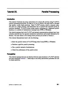
Figure 1: Reachability search from pivot p. computations. Such computations are coordinated by logical objects called synchronizers. A HipG parallel program is composed automatically from the sequential-like components provided by the user: pieces of work on graph nodes and synchronizers that initiate such work. The basic model and interface of HipG are explained in Section 2. One of the examples used there implements the bulk synchronous parallel (BSP) [14] model, which thus can be easily expressed in HipG. The two sections that follow detail advanced uses of HipG. The HipG model supports, but is not limited to, creating divide-and-conquer graph algorithms, as synchronizers can spawn sub-synchronizers to solve graph sub-problems. In Section 3 we show how to implement a divide-and-conquer parallel decomposition of a graph into strongly-connected components. In this paper we extend the model of HipG [13] with the support for execution and implementation of algorithms operating on graphs that are generated on-the-fly. Section 4 presents how we used this new feature to create a distributed model checker: we implemented a distributed cycle detection algorithm [15]. Although the user must be aware that a HipG program runs in a distributed environment, the code is high-level: explicit communication is not exposed by the API, nor are the algorithms tied to graph representations. Parallel composition is done in a way that does not allow race conditions, so that no locks or thread synchronization code have to be implemented by the user. These facts, coupled with the use of an object-oriented language, makes for an easy-to-use, but expressive, language to code parallel graph algorithms. We implemented HipG in Java. In Section 5 we discuss this choice as well as other implementation details, such as layout of the data structures used to store graphs (represented explicitly or generated on-the-fly) and organization of a worker. We evaluate performance of HipG in Section 6 on algorithms introduced in Sections 2-4. Using our newlybuilt cluster, DAS-4, we processed graphs of size of the order of 1010 (a magnitude larger than those used in [13]), and obtained good performance. The HipG code of the strongly connected components decomposition in HipG is an order of magnitude shorter than the hand-optimized C/MPI version of this program and three times shorter than the corresponding implementation in PBGL—See Section 7 for a discussion of the related work in the field of distributed graph processing. HipG’s current limitations and future work are discussed in the concluding Section 8.

2. BASIC HipG MODEL AND API The input to a HipG program is a directed graph. HipG partitions the graph into equal-size chunks. A chunk is a set of graph nodes and their outgoing edges; in other words, edges are co-located with their source nodes. Undirected edges are modeled as two directed edges. Each node is an object con-

interface MyNode extends Node { public void visit(); } class MyLocalNode implements MyNode extends LocalNode { boolean visited = false; public void visit() { if (!visited) { visited = true; for (int i=0; hasNeighbor(i); i++) neighbor(i).visit(); } } } Figure 2: Reachability search in HipG. taining arbitrary data and uniquely identified, for example by a pair (chunk, index). The target node of an edge is called a neighbor or a successor. Chunks are given to workers who are responsible for processing nodes that belong to them. Graphs are typically processed by following their structure, i.e. the node-edge relationship. For example, an algorithm may start processing at a pivot node, then process its neighbors, the neighbors’ neighbors, etc., until no nodes are left to be processed. Figure 1 illustrates such a computation of a set of nodes reachable from a pivot. This fine-grained structure-driven graph processing is the most basic ”primitive” of HipG. It is realized by providing the user with a unified interface to executing methods on local and non-local nodes, and a seamless access to a node’s list of neighbors. Reachability search. Figure 2 displays the reachability search in HipG in Java. First, a node interface is defined, MyNode, telling HipG which methods can be executed on remote nodes. In general, methods listed in the node interface can be executed on any graph node of which the unique identifier is known. The MyLocalNode the node implementation. Each node has a flag that denotes whether it has been visited. The visit() method visits an unvisited node and its neighbors. The parts underlined in the code are provided or required by HipG, the remaining parts were created by the user. There are several essential observations to be made about the code in Figure 2. First, no locks or other methods of synchronization were needed; the exclusive access to the node is assured by the framework. Lack of synchronization makes the code look sequential and therefore easy to program; nevertheless, the user must be aware that the code will execute in a parallel setting: the order in which methods execute cannot be predicted and relied upon in the algorithm. Even on a single processor, HipG might reorder node methods calls to prevent stack overflow. Second, the layout of the graph data structures is not exposed to the user; in fact, not only may the actual data structure vary in various graph implementations, but parts of it might not even be created yet (see Section 4). Finally, the user did not need to provide different handling of local and non-local neighbors: access to all graph’s nodes is unified. All these facts make HipG node methods easy to read and high-level: the code reflects the algorithm behind it. The algorithm in Figure 2 is initiated at the pivot node and terminates when all reachable nodes have been processed. In HipG this is written as:

pivot.visit(); barrier();

class BFS extends Synchronizer { QueueQ = new Queue(); int localQsize; public BFS(MyLocalNode pivot) { if (pivot != null) Q.add(pivot); localQsize = Q.size(); }

This code is, in fact, the simplest example of a synchronizer, a logical object that manages distributed computations. The three basic operations of a synchronizer are: (i) Initiating multiple distributed computations that execute in parallel or in sequence. For example, the call to pivot.visit() starts a wave of visit() method calls illustrated in Figure 1.

public void run() { int depth = 0; do { for (int i = 0; i < localQsize; i++) Q.pop().found(this, depth); depth++; barrier(); localQsize = Q.size(); } while (GlobalQsize(0) > 0); } @Reduce public long GlobalQsize(long partialQsize) { return partialQsize + localQsize; }

(ii) Waiting for issued computations to terminate by calling a barrier(). The barrier blocks the synchronizer until all computations initiated by this synchronizer have completed. For example, the barrier after pivot.visit() blocks until all reached nodes have been visited and there are no visit()’s in transfer. (iii) Computing global results of distributed computations e.g. a globally elected pivot, or a size of a set of nodes partitioned between workers (see the next example). One can imagine a synchronizer as an ”agent” (or an instance of the synchronizer) on each worker that manages distributed graph computations on behalf of the user. In HipG, the user writes a single-threaded program while automatic parallelization is provided by the library. Breadth-first search. Figure 3 shows the breadth-first search implemented in HipG. Its major part is the BFS synchronizer, which executes on each worker. BFS maintains a queue Q of nodes in the current layer, partitioned between the workers. The constructor adds the pivot to the queue at the worker that owns the pivot. The run method loops over the nodes in the current layer, and appends their unvisited neighbors to Q in the method found (not shown), in this way building the new layer. Note that the new elements may be added to queues on other workers. The barrier blocks until the new layer is fully created. Afterwards, the GlobalQsize method computes the global size of the new layer, and BFS terminates when all layers have been processed. Without the Reduce annotation, the call to GlobalQsize would be a regular method call returning the size of the local queue. With the annotation, it is a global reduce operation, which blocks until the sum of the sizes of all queues is computed. A single call to a reduce operation combines a partial result, supplied as an argument, with local data in a synchronizer and returns the combined value. The final value is a result of a chain of applications of the reduce method by all workers: each worker applies the reduce operation to a value from another worker, while the initiator applies it to the value supplied by the user. We note that (i) each worker executes the reduce method exactly once, (ii) the execution blocks until the result of the reduction is obtained, (iii) the final result is consistent across all workers, and, most importantly, (iv) the order of execution of reduce operations cannot be predicted and relied upon in the user’s code. We note that synchronizers only use high-level communication routines such as barriers and reduce operations. No other synchronization mechanisms are needed, even if there are multiple synchronizers per worker. Conceptually, the framework executes each run method sequentially, with ex-

} Figure 3: Breadth-first search in HipG. clusive access to the synchronizer’s data structures, and independently of other synchronizers. We observe that BFS alternates computation with global synchronization. Such algorithms are called bulk synchronous parallel (BSP) [14]. Lifting to parallel applications. In this section we described and gave examples of the two components of a HipG program that are defined by the user: node methods representing graph computations, and synchronizers orchestrating these computations. The two components are lifted automatically by HipG into a parallel application for a distributed-memory machine. At compile-time HipG translates method calls on non-local graph nodes into asynchronous messages. Since messages are asynchronous, methods do not return values. Returning a value of a method can be realized by sending a message back to the source, although, typically, the mechanism of computing global results by reduction is more efficient. All executions of methods on nodes, and messages representing them, form distributed graph computations managed by synchronizers. Each synchronizer is represented at each worker: each instance stores local state of computations and can manage local computations by communicating with other instances (this is also illustrated later in this paper in Figure 8). Each synchronizer has a unique id, determined on spawn, and consistent across all its instances. A typical HipG graph application starts by obtaining a graph, creates a synchronizer and waits until it terminates. In the two following sections we discuss more advanced programming with HipG.

3.

DIVIDE-AND-CONQUER IN HipG

Divide-and-conquer graph algorithms divide computations on a graph into several sub-computations on sub-graphs. HipG enables creation of sub-algorithms by allowing synchronizers to spawn any number of sub-synchronizers. Therefore, a HipG algorithm is, in fact, a tree of executing synchronizers, and thus a hierarchy of distributed algorithms. Synchronizers can manage child synchronizers, for example wait for child termination. Unless explicitly synchro-

FB(V ): p = pick a pivot from V F = FWD(p) B = BWD(p) Report (F ∩ B) as SCC In parallel: FB(F \ B) FB(B \ F ) FB(V \ (F ∪ B))

V F

p

B

Figure 4: Divide-and-conquer SCC-decomposition. nized, all synchronizers execute independently and in parallel. The user starts a graph algorithm by explicitly creating and spawning the root synchronizer. The system terminates when all synchronizers terminate. We illustrate divide-andconquer graph algorithms in HipG with an example of decomposition into strongly-connected components. Strongly-connected components. A strongly connected component (SCC) of a directed graph is a maximal set of nodes S such that there exists a path in S between any pair of nodes in S. We briefly describe FB [16], a divide-andconquer graph algorithm for computing SCCs, and sketch its implementation in HipG. The concept is explained in Figure 4. FB partitions the problem of finding SCCs of a set of nodes V into three sub-problems on three disjoint subsets of V . First an arbitrary pivot node is selected from V . Two sets F and B are computed as the sets of nodes that are, respectively, forward reachable and backward reachable (i.e. reachable in the transposed graph) from the pivot. The set F ∩ B is an SCC. All SCCs remaining in V must be entirely contained either within F \ B or within B \ F or within the complement set V \ (F ∪ B). The crucial part of a synchronizer FB is displayed in Figure 5. First, a global pivot is selected from V with the SelectPivot reduce operation. The pivot owner initializes forward and backward reachability searches that create sets F and B in V by flagging the reached nodes and storing them in separate queues. After F and B are fully computed, three sub-synchronizers are spawned to solve three sub-problems on F \ B, B \ F and V \ (F ∪ B). To label sets of nodes uniquely and consistently across all workers, the synchronizer’s unique identifier was utilized. We note that this algorithm uses a transposed graph; the transpose has to either be provided by the user or can be created by HipG. The HipG interface contains counterpart routines that work on a transpose, prefixed with in, for example inNeighbor. Most importantly, we observe that Figure 5 elegantly reflects the algorithm in Figure 4. A corresponding C/MPI application (see Section 6) has over 1700 lines of code that entirely obscures the algorithm, the PBGL implementation has 341 lines, while the entire FB in HipG is only 113 lines.

4. ON-THE-FLY GRAPH ALGORITHMS Encapsulating graph data structures and exposing only a high-level graph interface to the user, makes HipG highly malleable. Not only are algorithms not tied to particular graph representations, but also graphs can be created onthe-fly, i.e. during execution: a node is created on first access to it. This allows overlapping graph creation with computation for speed, and is essential in cases when the algorithm

class FB extends Synchronizer { ... public void run() { MyNode pivot = SelectPivot(null); if (pivot == null) return; if (pivot.isLocal()) { pivot.fwd(this, 2∗getId()); pivot.bwd(this, 2∗getId()+1); } barrier(); spawn(new FB(F \ B)); spawn(new FB(B \ F )); spawn(new FB(V \ (F ∪ B))); } } Figure 5: FB algorithm in HipG. only requires a part of the graph to execute, while the entire graph would not fit the memory. To execute an on-thefly algorithm the user only provides a definition of a next neighbor function prior to execution. Using this feature we implemented a distributed model checker, which otherwise might have taken months to develop from scratch. Distributed model checking. Model checking [4] is a widely-used technique that allows automatic verification of properties of computer programs (models) by systematically enumerating and examining their state spaces. The major problem this technique is facing is the state explosion: the state space grows exponentially with the number of variables or processes in the program to be checked. One way of alleviating this problem is to use distributed-memory model checkers, which make use of memories of multiple machines, but also render model checking algorithms more challenging. Such programs exist (see Section 7) and are typically large projects; the high-level API of HipG allows to vastly speed up development and try new algorithms with little effort. We implemented SpinJadi, a distributed model checker based on SpinJa2 [17], a recently developed clean Java reimplementation of Spin [5], the state-of-the-art sequential model checker. The input to the model checker is a Promela [5] file, which represents a multithreaded program augmented with assertions and a property to be checked. In general, model checking algorithms generate the state space of the model, while checking certain properties of generated states. In this section, a state of a program corresponds to a graph node, a state space corresponds to a graph, and checking properties of the state space to a graph algorithm. Two algorithms play a major role in distributed enumerative LTL3 model checking; SpinJadi invokes one of them, depending on the options supplied by the user. The on-thefly visitor is implemented similarly to the code in Figure 2, but augmented with safety checks (assertions, deadlocks) on visited states. The states are generated and checked until an error is found or the state-space is exhausted. The second algorithm checks properties of infinite executions of the model (for example a property that a certain ”stable” state is 2

SpinJa rhymes with Ninja; SpinJadi rhymes with Jedi LTL stands for Linear Temporal Logic – properties in Spin(Ja)(di) are expressed with the natural notion of linear time, i.e. words such as next, until, always, eventually 3

interface MapNode extends Node { public void map(MAP algo, long propag); } class LocalMapNode extends LocalNode implements MapNode { long map = BOTTOM; public void map(MAP algo, long propag) { if (algo.accCycle) return; if (id() == propag) { algo.accCycle(); } else if (propag > map) { map = propag; if (accepting) propag = max(map, id()); for (int i = 0; hasNeighbor(i) && !algo.accCycle; i++) neighbor(i).map(algo, propag); } } }

1

class MAP extends Synchronizer { Graph g; MapNode pivot; int accNodes = 0; boolean accCycle = false;

6

public void run() { do { if (pivot != null) g.node(pivot).map(this, 0, NIL); barrier(); if (accCycle) break; accNodes = 0; for (MapNode node : g) { node.map = BOTTOM; if (node.accepting) { if (node.map < node.id()) node.accepting = false; else accNodes++; } } barrier(); } while (GlobalAccNodes(0) > 0); } @Notification public void accCycle() { accCycle = true; } @Reduce public long GlobalAccNodes(long s) { return s + accNodes; }

11

16

21

Figure 6: Node implementation in the MAP. eventually reached from any other state), which is more challenging. Brim et al. [15] show that this can be accomplished by searching for an accepting cycle. Namely, the Promela input file annotates certain states (graph nodes) as ”bad”, or accepting. Existence of an accepting cycle, i.e. a cycle that contains an accepting state, proves that the property under consideration does not hold. Therefore, the second algorithm is the distributed on-the-fly Maximal Accepting Predecessors (MAP) algorithm [15]. MAP assumes that the graph nodes have unique totally-ordered identifiers. It relies upon the observation that an accepting cycle exists if and only if there exists a node with itself as its maximal (with respect to id) accepting predecessor. Therefore, in each iteration, MAP computes the maximal accepting predecessor for each node. If one of the accepting nodes is its own maximal accepting predecessor, an accepting cycle is reported. Otherwise, nodes which cannot be on an accepting cycle are discarded. The algorithm is described in detail and its correctness proved in [15]. Next, we briefly discuss how it was implemented in HipG. MAP. Figure 6 shows MAP’s ”primitive”: computation of the maximal accepting predecessor for each graph node. The identifier of the current maximal accepting predecessor is stored in the variable map. If a node receives its own identifier, an accepting cycle is reported. Otherwise, only map values greater than the current value are accepted for propagation. An accepting node propagates the maximum of its map and its identifier. The computation terminates when all map values stabilize. The global MAP algorithm is displayed in Figure 7. In each iteration, it computes all map values (lines 9–11). If an accepting cycle was reported, MAP terminates (line 12). Otherwise, it discards nodes that cannot be on a accepting cycle (map