Apr 11, 2009 - Probleme de Dirichlet pour les fonctions α-harmoniques sur les domaines coniques. Annales Mathematiques Blaise Pascal, 12:297 308, 2005.
Hitting half-spaces by Bessel-Brownian di�usions T. Byczkowski, J. Maªecki, M. Ryznar Institute of Mathematics and Computer Sciences, Wrocªaw University of Technology, Poland
arXiv:0904.1803v1 [math.PR] 11 Apr 2009
April 11, 2009
Abstract
The purpose of the paper is to �nd explicit formulas describing the joint distributions of the �rst hitting time and place for half-spaces of codimension one for a di�usion in Rn+1 , composed of onedimensional Bessel process and independent n-dimensional Brownian motion. The most important argument is carried out for the two-dimensional situation. We show that this amounts to computation of distributions of various integral functionals with respect to a two-dimensional process with independent Bessel components. As a result, we provide a formula for the Poisson kernel of a half-space or of a strip for the operator (I − ∆)α/2 , 0 < α < 2. In the case of a half-space, this result was recently found, by di�erent methods, in [6]. As an application of our method we also compute various formulas for �rst hitting places for the isotropic stable Lévy process.
1 Introduction Bessel processes appear in many important theoretical as well as practical applications. A systematic study, in the frame of one-dimensional di�usions, was initiated by H.P. McKean in [16]. Bessel processes, in particular, play an important role in a deeper understanding of the local time of the standard Brownian motion (see Ray-Knight Theorem in e.g. [20]). Their generalizations serve as various models in applications [10]. In our presentation, when considering Bessel processes, we follow the exposition of [20], Ch. XI. The purpose of the paper is to exploit a correspondence between harmonic measure of the operator in Rn (I − ∆)α/2 , 0 < α < 2, for a half-space or a strip and the joint distribution of the �rst hitting time and place for appropriate sets of codimension one for the (n + 1)-dimensional Bessel-Brownian di�usion, that is, the process Y(t) = (Rt(−α/2) , B n (t)), where Rt(−α/2) is one-dimensional BES (−α/2) process and B n is independent n-dimensional Brownian motion. Although we do not appeal to Molchanov-Ostrovski representation (see [19]) our results exemplify their principle that some jump Markov processes (here: isotropic stable and relativistic Lévy processes) can be regarded as traces of the appropriate Bessel-Brownian di�usions. With this regard we also mention the paper [2] where the eigenvalue problem for the Cauchy process in Rn was transformed into a kind of mixed eigenvalue problem for the Laplace operator in Rn+1 and also the work [7] which proposes to study n-dimensional non-local operators by means of (n + 1)-dimensional local operators. The paper is organized as follows. In Preliminaries (Section 2) we enclose some essentials about various special functions, indispensable in the sequel. We also provide a basic information about squared Bessel processes, Bessel processes and their hyperbolic and trigonometric variants, needed in the sequel. A detailed discussion of generalized Bessel processes is carried out in Appendix. 2000 MS Classi�cation: Primary 60J65; Secondary 60J60. Key words and phrases: Bessel processes, Bessel kernels, Riesz kernels, relativistic process, stable process, Poisson kernel, Green function, half-spaces. Research supported by Polish Ministry of Science and Higher Eduction grant N N201 3731 36
1
˜ ⊂ Rn In Section 3 we state our basic observation that the m-harmonic measure for some regular sets D for the n-dimensional α-stable relativistic process can be read from the joint distribution of the �rst exit ˜ ) for our Bessel-Brownian di�usion. The proof of time and place for the set D ⊂ Rn+1 (with the trace D this, intuitively apparent result, is postponed to Appendix. When m = 0 we obtain the same statement for the usual harmonic measure for the standard isotropic α-stable process. In Section 4 we �rst compute the joint distribution of the �rst hitting time and place for the vertical positive axis in the two-dimensional space for the process Y. Next, we deal with the same process Y but this time hitting two horizontal half-lines (−∞, −1] and [1, ∞). This is crucial for further purposes. We rely on stochastic calculus; in particular, we apply appropriate random change of time and compute various integral functionals of Bessel processes and generalized Bessel processes. The resulting formulas are, in the �rst case, in terms of modi�ed Bessel functions; in the second one - in terms of spheroidal wave functions. In the end of this section we apply our results to provide a purely probabilistic method of computing the Poisson kernel of the interval [−1, 1] for the standard isotropic α-stable process. In Section 5 we generalize previous results to multidimensional case. In the view of our principle from Section 3, the �rst part of Section 5 yields the formula for the Poisson kernel of a half-space for the operator (I − ∆)α/2 , 0 < α < 2, recently found in [6], using rather analytical methods. The second part gives a description of the Poisson kernel for a strip; also for the standard isotropic α-stable process.
2 Preliminaries In this section we collect some preliminary material. For more information on modi�ed Bessel functions, Whittaker's functions and hypergeometric functions we refer to [1] and [11]. For questions regarding Bessel processes, stochastic di�erential equations and one-dimensional di�usions we refer to [20] and to [17]. 2.1
Special functions
Modi�ed Bessel Functions Various potential-theoretic objects in the theory of the relativistic process are expressed in terms of modi�ed Bessel functions Iϑ and Kϑ . For convenience we collect here basic information about these functions. The modi�ed Bessel function Iϑ of the �rst kind is de�ned by (see, e.g. [11], 7.2.2 (12)):
Iϑ (z) = where ϑ ∈ R. The
∞ � � � z �ϑ X z 2k
2
k=0
2
1 , k!Γ(k + ϑ + 1)
z ∈ C \ (−R+ ),
(1)
modi�ed Bessel function of the third kind is de�ned by (see [11], 7.2.2 (13) and (36)): π [I−ϑ (z) − Iϑ (z)] , ϑ ∈ / Z, 2 sin(ϑπ) � � ∂Iϑ n 1 ∂I−ϑ Kn (z) = lim Kϑ (z) = (−1) − , ϑ→n 2 ∂ϑ ∂ϑ ϑ=n
(2)
Kϑ (z) =
n ∈ Z.
(3)
We will also use the following integral representations of the function Kϑ (z) ([11], 7.11 (23) or [14], 8.432 (6)): Z ∞ z2 −ϑ−1 ϑ (4) Kϑ (z) = 2 z e−t e− 4t t−ϑ−1 dt, 0
where > 0, | arg z| < In the sequel we will use the asymptotic behavior of Iϑ , as a function of real variable r: � r �ϑ 1 Iϑ (r) ∼ , r → 0+ , = Γ(ϑ + 1) 2
1 we have (6)
Iϑ (r) = (2πr)1/2 er [1 + E(r)] , where E(r) = O(r−1 ), r → ∞.
Con�uent hypergeometric function and Whittaker's functions The Laplace transforms of some additive functionals of Bessel processes are given in terms of the Whittaker's functions. We introduce some basic notation and properties of these functions. The con�uent hypergeometric function is de�ned by ∞ X (a)k z k Φ(a, b; z) = , (c)k k!
b 6= 0, −1, −2, . . . ,
k=0
where z is a complex variable, a and b are parameters. Here (a)k = Γ(a + k)\Γ(a) denotes the Pocchamer symbol. For | arg z| < π and b 6= 0, ±1, ±2, . . . we de�ne a new function
Ψ(a, b; z) =
Γ(1 − b) Γ(c − 1) 1−b Φ(a, b; z) + z Φ(1 + a − b, 2 − b; z) Γ(1 + a − b) Γ(a)
con�uent hypergeometric function of the second kind. The Whittaker's function of the �rst and the second kind are de�ned respectively by called the
Mκ, µ (z) = z µ+1/2 e−z/2 Φ(1/2 − κ + µ, 2µ + 1; z), Wκ, µ (z) = z µ+1/2 e−z/2 Ψ(1/2 − κ + µ, 2µ + 1; z),
(7)
| arg z| < π.
(8)
The con�uent hypergeometric function of the second kind satis�es the relation
Ψ(a, b; z) = z 1−b Ψ(1 + a − b, 2 − b; z),
| arg z| < π,
which implies that (9)
Wκ, µ (z) = Wκ, −µ (z). The following asymptotic formula ([1], 13.5.8 p. 508), valid for 1 < 0 and x > 0, the unique strong solution
dZ(t) = 2
p
|Z(t)|dβ(t) + δ dt ,
Z(0) = x ,
is called the square of δ -dimensional Bessel process started at x and is denoted by BESQδ (x). δ is the dimension of BESQδ . The square root of BESQδ (a2 ), a > 0, is called the Bessel process of dimension δ started at a and is denoted by BES δ (a). We introduce also the index ν = (δ/2) − 1 of the corresponding process, and write BESQ(ν) instead of BESQδ if we want to use ν instead of δ . The same convention applies to BES (ν) . For ν > −1, the semi-group BESQ(ν) (x) has a transition density function (ν)
qt (x, y) = and
1 � y �ν/2 −(x+y)/2t √ e Iν ( xy/t) 2 x
(ν)
for
x>0
qt (0, y) = (2t)−ν−1 t−(ν+1) Γ(ν + 1)−1 y ν e−y/2t .
(18) (19)
Iν denotes here the modi�ed Bessel function of the �rst kind. It is well known that for −1 < ν < 0 the point 0 is re�ecting; for ν > 0 the point 0 is polar. The in�nitesimal generator of BESQδ is equal on C 2 (0, ∞) to the operator 2x
d2 d +δ . 2 dx dx 4
(20)
If X is a BESQδ (x), then for any c > 0, the process c−1 X(ct) is a BESQδ (x/c). Next, we begin with introducing the two dimensional process Y = (Y1 , Y2 ) with independent components as Y1 being the squared BESQ(−α/2) process and Y2 - the standard Brownian motion. Equivalently, Y = (Y1 , Y2 ) satis�es the following stochastic diferential equations p � ˜1 + (2 − α)dt dY1 = 2 |Y1 |dB (21) ˜2 , dY2 = dB
˜1 , B ˜2 ) denote the standard two dimensional Brownian motion (E B ˜i (t) = 0, E B ˜ 2 (t) = t for where (B i i = 1, 2), and where 0 < α < 2, Y1 (0) = y1 > 0 and Y2 (0) = y2 , with y2 ∈ R. It is well-known that Y1 > 0. Consequently, the absolute value in the �rst equation of (21) can be discarded. Also, for −1 < ν < 0, the point 0 is (instantaneously) re�ecting and the process Y1 is (pointwisely) recurrent. ˜1 , B ˜2 ). We consider another Let (B1 , B2 ) be the standard Brownian motion in R2 independent from (B (−α/2) pair (X1 , X2 ) of independent squared Bessel processes BESQ de�ned by the following system of stochastic di�erential equations � √ dX1 = 2√X1 dB1 + (2 − α) dt (22) dX2 = 2 X2 dB2 + (2 − α) dt, such that X1 (0) = x1 , X2 (0) = x2 , where x1 , x2 > 0. We de�ne a function f = (f1 , f2 ) : R2 → R2 by f (x1 , x2 ) = (4x1 x2 , x2 −x1 ). Let (Z1 , Z2 ) = f (X1 , X2 ). Using Itô formula we obtain
dZ1 = 4X2 dX1 + 4X1 dX2 p p = 4X2 2 X1 dB1 + 4X2 (2 − α)dt + 4X1 2 X2 dB2 + 4X1 (2 − α)dt p p p = 4 X1 X2 (2 X2 dB1 + 2 X1 dB2 ) + 4(X1 + X2 )(2 − α)dt p p p = 2 Z1 (2 X2 dB1 + 2 X1 dB2 ) + 4(X1 + X2 )(2 − α)dt, p p dZ2 = −2 X1 dB1 + 2 X2 dB2 . Observe that if we put
p p X2 dB1 + 2 X1 dB2 , p p = −2 X1 dB1 + 2 X2 dB2 ,
dU1 = 2 dU2
then the process (U1 , U2 ) is a continuous martingale starting from 0 such that
dhU1 i(t) = 4(X1 + X2 )dt, dhU2 i(t) = 4(X1 + X2 )dt, dhU1 , U2 i(t) = 0. If we de�ne the following integral functional
Z
t
A1 (t) = 4
(X1 (s) + X2 (s))ds 0
and its generalized inverse function
σ1 (s) = inf{t > 0 : A1 (t) > s}, then we get (see [17] Theorem 7.3 p. 86) that the process (U1 (σ1 (s)), U2 (σ1 (s))) is a standard 2dimensional Brownian motion (β1 , β2 ). Consequently we obtain p dZ1 ◦ σ1 = 2 |Z1 ◦ σ1 |dβ1 + (2 − α)dt,
dZ2 ◦ σ1 = dβ2 . d
This means that Y = Z ◦ σ1 , where Y = (Y1 , Y2 ) is the process de�ned by (21). 5
Time change of generalized Bessel processes In this section we consider the process X = (X1 , X2 ) given by the following stochastic di�erential equations p 2−α dX1 = |1 − X12 | dB1 − X1 dt 2 (23) p 2−α dX2 = |X22 − 1| dB2 + |X2 | dt, 2 such that X1 (0) = x1 , X2 (0) = x2 , where |x1 | 6 1 and x2 > 1. Here B1 , B2 are two independent standard Brownian motions in R. It follows that that for |X1 (0)| 6 1 we have |X1 (t)| 6 1 for all t > 0. The boundary points 1 and (−1) are instantaneously re�ecting. Analogously, X2 (t) > 1, whenever X2 (0) > 1 and the boundary point 1 is also instantaneously re�ecting. For justi�cation of these statements, see Appendix. The �rst process is a version of Legendre process; the second one - of hyperbolic Bessel process. Obviously the processes X1 , X2 are independent. Moreover, the generators of the processes are given by
G1 = G2 =
1 − x2 d2 2−α d − x , 2 2 dx 2 dx 2−α d x2 − 1 d2 + x , 2 dx2 2 dx
(24) (25)
respectively. Let h = (h1 , h2 ) : R2 −→ R2 by h1 (x1 , x2 ) = (1 − x21 )(x22 − 1) and h2 (x1 , x2 ) = x1 x2 . We de�ne the process Z = (Z1 , Z2 ) = h(X1 , X2 ). Using Itô formula we get
dZ1 = −2 X1 (X22 − 1) dX1 + 2 X2 (1 − X12 ) dX2 − (X22 − 1) (1 − X12 ) dt + (X22 − 1) (1 − X12 ) dt q q p 2 = 2 |Z1 |(−X1 X2 − 1 dB1 + X2 1 − X12 dB2 ) + (2 − α)(X22 − X12 ) dt, dZ2 = X2 dX1 + X1 dX2 q q = (X2 1 − X12 dB1 + X1 X22 − 1 dB2 ). Observe that for
dW1 dW2
q q 2 = −X1 X2 − 1 dB1 + X2 1 − X12 dB2 , q q 2 = X2 1 − X1 dB1 + X1 X22 − 1 dB2 ,
we have dhW1 i(t) = dhW2 i(t) = X22 − X12 and dhW1 , W2 i(t) = 0. Thus for
Z A2 (t) =
t
(X22 (s) − X12 (s)) ds
(26)
0
and σ2 = inf{t > 0 : A2 (t) > s} we get that (W1 (σ2 (t)), W2 (σ2 (t))) is a standard two dimensional Brownian motion (β1 , β2 ) and consequently we have p dZ1 ◦ σ2 = 2 Z1 ◦ σ2 dβ1 + (2 − α)dt,
dZ2 ◦ σ2 = dβ2 . d
Comparing this with (21) gives Y = Z ◦ σ2 .
6
3 Relativistic stable processes and Bessel-Brownian di�usions Assume that 0 < α < 2. A Lévy process X m (t), living in Rn , is called the α-stable process with parameter m ≥ 0 if its characteristic function is given by
E 0 ehz,X
m (t)i
= emt e−t(|z|
2 +m2/α )α/2
,
relativistic stable
z ∈ Rn .
For m = 0 we obtain the standard isotropic α-stable process. The generator of X m (t) is given by mI − (m2/α I − ∆)α/2 . For more information about relativistic processes we refer the reader to [8] and [22]. ˜ ⊂ Rn we de�ne τ ˜ = inf{t > 0; X m (t) ∈ ˜ . The λ-harmonic measure of the set For an open set D / D} D ˜ D is de�ned as x −λτD ˜ PDλ,m 1A (X m (τD˜ ))], ˜ < ∞; e ˜ (x, A) = E [τD where A is a Borel subset of Rn . In this paper we are interested only in the case λ = m and we will denote m . Note that the relativistic process killed at an independent exponential time with expectation PDm,m as PD ˜ ˜
1/m has the generator equal to −(m2/α I −∆)α/2 . Therefore PDm ˜ can be regarded as the harmonic measure 2/α α/2 ˜ of D for the operator −(m I − ∆) . If this harmonic measure is absolutely continuous with respect ˜ c we call the corresponding density the m-Poisson kernel of D ˜ and denote to the Lebesgue measure on D m (˜ by PD ˜ x, ·). Next, let Y(t) = (Y1 (t), B n (t)) be an (n + 1)-dimensional di�usion with independent components, where Y1 (t) is BES (−α/2) and B n (t) = (B2 (t), B3 (t), . . . , Bn+1 (t)) is the standard Brownian motion in Rn . The following proposition exhibits the fact that �nding m-harmonic measures is equivalent to �nding some hitting distributions of the process Y(t).
Proposition 3.1. Let D˜ ⊂ Rn be open. Assume that F = Rn \ D˜ has the interior cone property at every point. Let D = Rn+1 \ ({0} × F ). Let x = (0, x˜) ∈ {0} × D˜ . De�ne τD = inf{t > 0; Y(t) ∈/ D} and assume that P x (τD < ∞). Then for every Borel A ⊂ Rn we have x − PDm ˜ (x, A) = E [e
m2/α τD 2
; B n (τD ) ∈ A].
The conclusion is valid also for m = 0, that is for the harmonic measure for the standard isotropic α-stable process. The proof of the above proposition is provided in the Appendix.
4 Hitting distributions in R2 We begin this section with considering two dimensional case, which is crucial for further computations in higher dimensions. 4.1
Hitting distribution of a positive vertical half-line in
R2
We compute here the joint distribution of the �rst hitting time and place of the positive vertical axis (−α/2) (−α/2) for the process (Rt , B(t)) with independent components, where Rt is a BES (−α/2) process and B(t) is the standard Brownian motion. We always assume here that 0 < α < 2. De�ne the following two sets
H = {(x1 , x2 ) ∈ [0, ∞) × [0, ∞) : x1 > 0}, D1 = {(y1 , y2 ) ∈ R × [0, ∞) : (y1 = 0) ∧ (y2 > 0)}c . (−α/2)
Let denote by τD1 the �rst exit time of the process (Rt , B(t)) from the set D1 , i.e. τD1 = inf{t > (−α/2) (−α/2) (−α/2) 0 : (Rt , B(t)) ∈ / D1 }. Observe that the BES (a) process Rt hits the 0 exactly when 7
(−α/2)
BESQ(−α/2) (a2 ) process (Rt )2 hits the 0. Therefore, we consider, as in (21) processes (Y1 , Y2 ) with (−α/2) 2 Y1 = (R ) and Y2 = B . We thus have / D1 }. τD1 = inf{t > 0 : Y (t) ∈ We denote by τH the �rst exit time of the process X = (X1 , X2 ) with independent BESQ(−α/2) components, as de�ned by (22), from the set H , i.e.
τH = inf{t > 0 : X(t) ∈ / H} = inf{t > 0 : X1 (t) = 0}. Recall that f (x1 , x2 ) = (4x1 x2 , x2 − x1 ).
f
−→
Figure 1: Simulated paths of X = (X1 , X2 ) and image Y = (Y1 , Y2 ) under mapping f .
Lemma 4.1. The distribution of (τD1 , Y (τD1 )) with respect to P (y1 ,y2 ) is the same as the distribution of (A1 (τH ), f (X(τH ))) with respect to (x1 , x2 ), where f (x1 , x2 ) = (y1 , y2 ). R Proof. We recall that A1 (t) = 4 0t (X1 (s) + X2 (s)) ds. It is easy to see that f (H) = D1 and that the
function f is bijective on H . Moreover, from the time change property proved in the previous subsection we get d f (X(σ1 (t)))=Y (t), where the equality in distribution is meant for the underlying processes. Hence in order to prove the lemma we may and do assume that f (X(σ1 (t))) = Y (t), t ≥ 0. We have
τD1
= inf{t > 0 : Y (t) ∈ / D1 } = inf{t > 0 : f (X(σ1 (t))) ∈ / D1 } = inf{t > 0 : X(σ1 (t)) ∈ / H} = inf{A1 (u) > 0 : X(u) ∈ / H} = A1 (τH )
and
Y (τD1 ) = f (X(σ1 (τD1 ))) = f (X(σ1 (A1 (τH )))) = f (X(τH )) = (0, X2 (τH )). The proof of the main result of this subsection is based on well-known formulas describing distributions of some integral functionals of quadratic Bessel processes, stated here in the following two lemmas. For convenience of the reader we include proofs. 8
Lemma 4.2. Let X be a BESQ(ν) process with ν > −1. Then for x > 0 the following holds: E
x
�
� √ � 2Z t � � � � r �ν/2 λ(x+r) λ xrλ λ coth(tλ) − 2 exp − X(s)ds ; X(t) ∈ dr = Iν . e 2 0 x 2 sinh(tλ) sinh(tλ)
For x = 0 we obtain � � � � 2Z t λ X(s)ds ; X(t) ∈ dr = E exp − 2 0 0
λr 1 rν λν+1 e− 2 coth(tλ) . ν+1 Γ(1 − ν) (2 sinh(tλ))
Proof. The above follows directly from the formula for the distribution of the corresponding integral (ν)
functional for the quadratic Bessel Bridge BESQ1 (x, y) which can be found, e.g. in [20], Ch. XI, Corollary 3.3, p. 465: �√ � xrλ �� � �I � � 2Z 1 ν sinh(λ) λ (x + r) λ √ X(s)ds = exp (1 − λ coth(λ)) , Q(ν),1 exp − x,y 2 0 sinh(λ) 2 Iν ( xr) (ν),1
(ν)
where Qx,y is the distribution of the quadratic Bessel Bridge BESQ1 (x, y). The above formula, the scaling properties of BESQ(ν) processes and the formula (18) for the density of BESQ(ν) give the �rst formula of the Lemma. The second formula is obtained from the �rst one by limiting procedure as b → 0, taking into account (5)
Lemma 4.3. Let X be a x > b > 0 we have
BESQ(ν)
process with ν > −1. De�ne τb = inf{s : X(s) = b}. Then for
λ2 uγ (x) = E [exp(−γτb − 2 x
Z
τb
X(s) ds)] = 0
x−(ν+1)/2 W−γ/2λ, |ν|/2 (λx) b−(ν+1)/2 W−γ/2λ, |ν|/2 (λb)
.
For −1 < ν < 0 and b = 0 we obtain for x > 0 λ2 E [exp(−γτ0 − 2 x
Z 0
τ0
Γ( ν+1+λ/2 ) −(ν+1)/2 x W−γ/2λ, |ν|/2 (λx). X(s) ds)] = (ν+1)/22 λ Γ(|ν|)
(27)
Proof. By the form of the generator of the process X (20) and the general theory of Feynman-Kac semigroups [9] we infer that the function uγ (x) satis�es for x > b the following diferential equation
2x
d2 uγ (x) duγ (x) + 2(ν + 1) − ((λ2 x)/2 + γ) uγ (x) = 0 . dx2 dx
(28)
The two linearly independent solutions of (28) are of the form
ψ(x) = x−(ν+1)/2 M−γ/2λ,|ν|/2 (λx)
and
φ(x) = x−(ν+1)/2 W−γ/2λ,|ν|/2 (λx) ,
where M−γ/2λ,|ν|/2 and W−γ/2λ,|ν|/2 are Whittaker's functions de�ned in (7) and (8). Taking into account the fact that the function uγ (x) is bounded and uγ (b) = 1 we obtain the �rst formula. The second formula follows from the �rst one and the asymptotic formula (10) which gives ! Γ(|ν|) λν bν + O(1) . b−(ν+1)/2 W−γ/2λ, |ν|/2 (λb) = λ(1−ν)/2 b−ν e−λb/2 ν+1+λ/2 Γ( ) 2 Hence, we obtain
lim b−(ν+1)/2 W−γ/2λ, |ν|/2 (λb) = λ(ν+1)/2
b→0
which proves the second formula.
9
Γ(|ν|) Γ( ν+1+λ/2 ) 2
,
Theorem 4.4. For (R0(−α/2) , B(0)) = (z1 , z2 ) ∈ D1 , z1 > 0 and r > 0 we have E
(z1 ,z2 )
� � 2 − λ2 τD1 e ; B(τD1 ) ∈ dr = α
α
(|z| + z2 ) 4 (|z| − z2 ) 2 2
3α 4
Z
Γ( α2 )rα/4
∞
e−(|z|+r)s (s2 − λ2 )α/4 I−α/2
�√ p � p 2r |z| + z2 s2 − λ2 ds.
λ
For z1 = 0 and z2 = u < 0 we get E
(0,u)
�
�
2
− λ2 τD1
e
; B(τD1 ) ∈ dr
sin(πα/2) π
=
�
−u r
�α/2
e−λ(r−u) . r−u
(29)
Proof. Let φ ∈ Cc∞ (0, ∞) and λ > 0. From Lemma 4.1 we obtain that E
(y1 ,y2 )
�
2
− λ2 τD1
e
� λ2 φ(Y (τD1 )) = E (x1 ,x2 ) [e− 2 A1 (τH ) φ(X2 (τH ))].
It is convenient to carry out our computations for λ/2 instead of λ. From the independence of the processes X1 and X2 and the fact that τH is determined only by X1 we get that Z λ 2 τH λ2 (x1 ,x2 ) (x1 ,x2 ) [exp(− (X1 (s) + X2 (s))ds)φ(X2 (τH ))] E [exp(− A1 (τH ))φ(X2 (τH ))] = E 8 2 0 � � Z Z λ2 τH λ2 t x1 x2 = E [exp(− X1 (s)ds) E exp(− ] X2 (s)ds)φ(X2 (t)) 2 0 2 0 t=τH Z Z ∞ λ2 τH = E x1 [exp(− X1 (s)ds) ψ(τH , x2 , r)φ(r)dr] 2 0 0 Z ∞Z ∞ w(t, x1 )ψ(t, x2 , r)φ(r)drdt, = 0
0
where
ψ(t, x, r) = E
x
w(t, x) = E
x
�
� 2Z t � � λ exp − X2 (s)ds ; X2 (t) ∈ dr 2 0
and
�
λ2 exp(− 2
Z
τH
X1 (s) ds) ; τH
� ∈ dt .
0
From Lemma 4.2, putting ν = −α/2, we obtain
ψ(t, x, r) = xα/4
λr−α/4 −λ (x+r) coth(tλ) 2 e I−α/2 2 sinh(tλ)
� √
xrλ sinh(tλ)
� .
To evaluate w(t, x) we apply the formula (27) from Lemma 4.3 putting again ν = −α/2. We obtain
λ2 E [exp(−γτH − 2 x
Z
τH
X1 (s) ds)] = 0
Γ( 12 − α4 + λ4 ) α/4−1/2 x W−γ/2λ, α/4 (λx). λ1/2−α/4 Γ(α/2)
(30)
Now we invert the formula (30) with respect to γ . Using (9) and the formula 25 p. 651 from [5] we obtain that � � � � Z xα/2 λ1+α/2 λ2 τH xλ cosh(tλ) w(t, x) = E x exp(− X1 (s) ds) ; τ ∈ dt = exp − dt. 2 0 2 sinh(tλ) 2α/2 Γ(α/2) sinh1+α/2 (tλ) 10
Combining all the above we get Z ∞ (x1 ,x2 ) w(t, x1 )ψ(t, x2 , r)dt P (λ, r) = 0 α
α
α
x12 x24 λ2+ 2 α 21+ 2 Γ( α2 )
=
Z
� � � � √ rx2 λ (x1 + x2 + r) coth(tλ) exp −λ I− α2 dt. α 2 sinh(tλ) sinh2+ 2 (tλ)
∞
r−α/4
0
After substituting λ coth(tλ) = 2s we get α
α
(x2 ) 4 (x1 ) 2 α 2 2 Γ( α2 )rα/4
Z
∞
e−(x1 +x2 +r)s ((2s)2 − λ2 )α/4 I−α/2
�√
rx2
� p (2s)2 − λ2 ds.
λ/2
Now taking 2λ instead λ we have
λ2 E (x1 ,x2 ) [exp(− A1 (τH ))φ(X2 (τH ))] 2 α Z α � √ p � (x2 ) 4 (x1 ) 2 ∞ −(x1 +x2 +r)s 2 2 α/4 2 − λ2 ds. e (s − λ ) I rx s = 2 2 −α/2 Γ( α2 )rα/4 λ Coming back to initial variables (y1 , y2 ) = (4x1 x2 , x2 − x1 ) and (y1 , y2 ) = (z12 , z2 ) we obtain q x1 + x2 = y1 + y12 = |z| , x1 = (|z| − z2 )/2 and x2 = (|z| + z2 )/2 . Finally
� � λ2 E (z1 ,z2 ) e− 2 τD1 ; B(τD1 ) ∈ dr = α
α
(|z| + z2 ) 4 (|z| − z2 ) 2 2
3α 4
Γ( α2 )rα/4
Z
∞
e−(|z|+r)s (s2 − λ2 )α/4 I−α/2
λ
From (5) we get that
lim z ν I−ν (xz) =
z→0
Consequently, for z1 = 0, z2 = u < 0 we get � � 2 (0,u) − λ2 τD1 E e ; B(τD1 ) ∈ dr =
=
4.2
�√ p � p 2r |z| + z2 s2 − λ2 ds.
2ν . Γ(1 − ν)xν
α
(−2u) 2 2α/2
Z
∞
3α 4
Γ( α2 )Γ(1 − α2 )2α/4 rα/2 λ � � sin(πα/2) −u α/2 e−λ(r−u) . π r r−u
2
Hitting distribution of two half-lines in
e−(r−u)s ds
R2
In this section we are interested in �nding the distribution of the �rst hitting time and place of two (−α/2) half-lines for the process (Rt , B(t)). De�ne the following two sets
G = {(x1 , x2 ) ∈ [−1, 1] × [1, ∞) : −1 < x1 < 1}, C1 = {(y1 , y2 ) ∈ R × [0, ∞) : (y1 = 0) ∧ (|y2 | > 1)}c .
11
(−α/2)
, B(t)) from the set C1 , i.e. τC1 = inf{t > and denote by τC1 the �rst exit time of the process (Rt (−α/2) 0 : (Rt , B(t)) ∈ / C1 }. As previously we can consider the processes Y = (Y1 , Y2 ) de�ned in (21) with Y1 = (R(−α/2) )2 and Y2 = B . We thus have τC1 = inf{t > 0 : Y (t) ∈ / C1 }. Denote by τG the �rst exit time of the process X = (X1 , X2 ) with independent BESQ(−α/2) components, as de�ned by (22), from the set G, i.e.
τG = inf{t > 0 : X(t) ∈ / G} = inf{t > 0 : |X1 (t)| = 1}. The function h was de�ned by h1 (x1 , x2 ) = (1 − x21 )(x22 − 1).
h
−→
Figure 2: Simulated paths of X = (X1 , X2 ) and image Y = (Y1 , Y2 ) under mapping h. Using the same arguments as in Lemma 4.1 we get the equality between distributions of (τC1 , Y (τC1 )) and (A2 (τG ), h(X(τG ))), where in this case the integral functional A2 (t) is given by Z t A2 (t) = (X22 (s) − X12 (s))ds 0 Z t (q1 (X1 (s)) + q2 (X2 (s)))ds, = 0
where q1 (x) = 1 − x2 and q2 (x) = x2 − 1. Notice that q1 (X1 (s)) > 0 and q2 (X2 (s)) > 0 almost surely.
Lemma 4.5. The distribution of (τC1 , Y (τC1 )) with respect to P (y1 ,y2 ) is the same as the distribution of (A2 (τG ), h(X(τG ))) with respect to (x1 , x2 ), where h(x1 , x2 ) = (y1 , y2 ). Now we state the main theorem of the section. We give a representation of the density of (τC1 , Y (τC1 )) in terms of spheroidal wave functions (see (36)).
Theorem 4.6. For (R0(−α/2) , B(0)) = (z1 , z2 ) ∈ C1 and r > x2 > 1 we have Z α/4+i∞ 1 1 ; B(τC1 ) ∈ dr = 2 m−ϑ, λ (x1 ) wλ (ϑ)φ↑ϑ, λ (x2 )φ↓ϑ, λ (r)dϑ, (31) E e (r − 1)α/2 2πi α/4−i∞ �p � �p � p p where x1 = 12 z12 + (z2 + 1)2 + z12 + (z2 − 1)2 , x2 = 21 z12 + (z2 + 1)2 − z12 + (z2 − 1)2 and the function mϑ, λ (·) is the solution of the following di�erential equation (z1 ,z2 )
�
2
− λ2 τC1
�
(1 − x2 )y 00 (x) − (2 − α)x y 0 (x) − (λ2 (1 − x2 ) + 2ϑ)y(x) = 0, 12
|x| < 1,
(32)
with boundary conditions mϑ, λ (−1) = 0, mϑ, λ (1) = 1. The functions φ↑ϑ, λ (·), φ↓ϑ, λ (·) are respectively increasing and decreasing independent positive solutions of the di�erential equation (r2 − 1)y 00 (r) + (2 − α)r y 0 (r) − (λ2 (r2 − 1) + 2ϑ)y(r) = 0,
r > 1.
(33)
satisfying limx→1+ φ↑ϑ, λ (x) = 0, limx→∞ φ↓ϑ, λ (x) = 0 and wλ (ϑ) =
2 (1 −
r2 )α/2−1 W {φ↑ϑ, λ , φ↓ϑ, λ }(r)
.
Proof. Let φ ∈ Cc∞ (1, ∞) and λ > 0. According to Lemma 4.5 we have (y1 ,y2 )
E
�
2
− λ2 τC1
e
� � � 2 − λ2 A2 (τG ) (x1 ,x2 ) e φ(Y (τC1 )) = E φ(h(X(τG ))) .
We de�ne the following functions � � Z λ2 t Ψλ (t, x, r) = Ex exp(− q2 (X2 (s))ds); X2 (t) ∈ dr , 2 0
x > 1, t > 0, r > 1,
and
� � Z λ 2 τG q1 (X1 (s))ds); X1 (τG ) = 1; τG ∈ dt , Wλ (t, x) = E exp(− 2 0 x
|x| 6 1, t > 0.
Moreover, for every ϑ > 0, we de�ne its Laplace transforms with respect to the variable t by Z ∞ mϑ, λ (x) = e−ϑt Wλ (t, x) dt, 0 Z ∞ Mϑ, λ (x, r) = e−ϑt Ψλ (t, x, r) dt. 0
Observe that ∞
Z mϑ, λ (x) =
e−ϑt Wλ (t, x) dt
0
� Z λ 2 τG = E X1 (τG ) = 1; exp(−ϑτG ) exp(− g1 (X1 (s))ds) 2 0 � � Z τG ∗ x g1 (X1 (s))ds) , = E X1 (τG ) = 1; exp(− x
�
0
where q1∗ (x) =
λ2 2 (1
− x2 ) + ϑ. Using the Schrödinger equation (see [9] Theorem 9.10) we get that (G1 mϑ, λ )(x) − q1∗ (x)mϑ, λ (x) = 0
(1 − x2 )m00ϑ, λ (x) − (2 − α)x m0ϑ, λ (x) − (λ2 (1 − x2 ) + 2ϑ)mϑ, λ (x) = 0. For x = −1 and x = 1 we have τG = 0 and consequently mϑ, λ (−1) = 0 and mϑ, λ (1) = 1. We have Z ∞ Mϑ, λ (x, r) = e−ϑt Ψλ (t, x, r) dt 0 � � Z ∞ Z λ2 t −ϑt x = e E exp(− q2 (X2 (s))ds); X2 (t) ∈ dr . 2 0 0 Observe that the function
� � Z λ2 t p(t, x, r) = E exp(− q2 (X2 (s))ds); X2 (t) ∈ dr , 2 0 x
13
t > 0;
x, r > 1,
(34)
is the transition density of one-dimensional di�usion with the generator
λ2 1 d2 u 2 − α du L2 u = (x2 − 1) 2 + x 2 − (x2 − 1)u. 2 dx 2 dx 2 From the general theory (see [5], Ch. II) we have that the ϑ-Green function of the di�usion is given by Z ∞ Gϑ (x, r) = e−ϑt p(t, x, r) dt = cλ (ϑ) · φ↑ϑ, λ (x)φ↓ϑ, λ (r), x < r, (35) 0
where φ↑ϑ, λ (x), φ↓ϑ, λ (x) are positive solutions of the di�erential equation
L2 u − ϑu = 0 such that φ↑ϑ, λ (x) is increasing and φ↓ϑ, λ (x) is decreasing and they satisfy the boundary conditions
limx→1+ φ↑ϑ, λ (x) = 0, limx→∞ φ↓ϑ, λ (x) = 0. The Wronskian of the pair (φ↑ϑ, λ (x), φ↓ϑ, λ (x)) is given by d ↓ φϑ, λ (x) − W {φ↑ϑ, λ , φ↓ϑ, λ } = φ↑ϑ, λ (x) dx
↓ d ↑ dx φϑ, λ (x)φϑ, λ (x)
and the function cλ (ϑ) is given by
cλ (ϑ) = wλ (ϑ)m(r) s0 (r) m(r). = W {φ↑ϑ, λ , φ↓ϑ, λ }(r) 1 = wλ (ϑ) 2 , (r − 1)α/2 where the function
wλ (ϑ) =
2 (r2 − 1)α/2−1 W {φ↑ϑ, λ , φ↓ϑ, λ }(r)
does not depend on r. Recall that τG depends only on X1 and the processes X1 and X2 are independent. Thus we easily obtain that the expression in the right hand side of (34) is equal to Z Z λ 2 τG λ2 t x1 x2 E [exp(− q1 (X1 (s))ds)E [exp(− q2 (X2 (s))ds)φ(X2 (t))]τG =1, X1 (τG )=1 ] = 2 0 2 0 Z ∞ Z ∞ = Wλ (t, x1 ) φ(r)Ψλ (t, x2 , r) dr dt Z0 ∞ Z ∞ 1 = φ(r) Wλ (t, x1 )Ψλ (t, x2 , r)dt dr. 1
0
Observe that
Z |mϑ, λ (x)| 6
∞
− 0 : Y(t) ∈ / Cn }. In order to describe the distribution of (τCn , Y(τCn )) we de�ne � � 2 − λ2 τC1 (z1 ,z2 ) e H(z1 , z2 , λ, r) = E ; B2 (τC1 ) ∈ dr , |r| > 1, where (z1 , z2 ) ∈ C1 . The integral representation of H(z1 , z2 , λ, r) is the main result of Section 4.2 (see the formula (31)). We de�ne
h(λ, y, σ ˜ ) = E y [e−
λ2 τ 2 Cn
; B n (τCn ) ∈ d˜ σ ], σ ˜ = (σ2 , . . . , σn+1 ) ∈ Rn , |σ2 | > 1.
In the next theorem we provide a formula for the (n − 1)-dimensional Fourier transform of h(λ, y, σ ˜ ), which entirely describes the distribution of (τCn , Y(τCn )).
Theorem 5.4. Let n ≥ 2. For y = (0, y2 , . . . , yn+1 ) such that |y2 | < 1 and z¯ ∈ Rn−1 we have Z
h(λ, y, σ ˜ )ei(¯σ,¯z ) d¯ σ = H(0, y2 ,
p |¯ y − z¯|2 + λ2 , σ2 ).
Rn−1
(42)
Here σ˜ = (σ2 , σ¯ ). Proof. Let f y2 (t, σ2 ) = E (0,y2 ) [τC1 ∈ dt, B2 (τC1 ) ∈ dσ2 ]. When n > 2 we observe that the density of the joint distribution of (τCn , B2 (τCn )) with respect to P (0,y2 ) is equal to f y2 (t, σ2 ). Let gt (¯ x) denote the density function of the distribution of (n − 1)-dimensional Brownian motion. Using the fact that the �rst exit time τCn depends only on Y1 and B2 we obtain
E y [τCn ∈ dt, Y(τCn ) ∈ dσ] = E y [τCn ∈ dt, B2 (τCn ) ∈ dσ2 , B3 (τCn ) ∈ dσ3 , . . . Bn+1 (τCn ) ∈ dσn+1 ] = E (0,y2 ) [τCn ∈ dt, B2 (τCn ) ∈ dσ2 ] gt (¯ y−σ ¯) = f y2 (t, σ2 ) gt (¯ y−σ ¯) . This implies that y
h(λ, y, σ ˜ ) = E [e
2
− λ2 τCn
; Y(τCn ) ∈ d˜ σ] =
Z
∞
e−
λ2 t 2
f y2 (t, σ2 ) gt (¯ y−σ ¯ )dt.
0
Hence, the formula for the (n − 1)-dimensional Fourier transform of h(λ, y, σ ˜ ) can easily be found Z Z ∞ Z Z ∞ 2 |¯ y −¯ z |2 +λ2 i(¯ σ ,¯ z) − λ2 t y2 i(¯ σ ,¯ z) 2 h(λ, y, σ)e d¯ σ= e f (t, σ2 ) gt (¯ y−σ ¯ )e d¯ σ dt = f y2 (t, σ2 ) e−t dt. Rn−1
0
Rn−1
p Next, observe that the last integral is equal to H(0, y2 , |¯ y − z¯|2 + λ2 , σ2 ). 21
0
Again, the following corollary is an immediate consequence of Theorem 5.4 and Proposition 3.1.
Corollary 5.5. Assume that n ≥ 2. Let C˜n ⊂ Rn be the strip {˜x ∈ Rn ; |x1 | < 1} ⊂ Rn . Then the (n − 1)-dimensional Fourier transform of m-Poisson kernel of C˜n for the relativistic α-stable process with parameter m ≥ 0 is given by Z
PCm y, σ ˜ )ei(¯σ,¯z ) d¯ σ ˜n (˜
Rn−1
= H(0, y1 ,
q
|¯ y − z¯|2 + m2/α , σ1 ) ,
where y˜ = (y1 , . . . , yn ) ∈ C˜n and σ˜ = (σ1 , σ¯ ) ∈ C˜nc . Note that the above formula for m = 0 provides the (n − 1)-dimensional Fourier transform of the Poisson kernel of the strip C˜n for the standard isotropic α-stable process. In the last part of this section we assume that 1 < α < 2. We consider a similar problem as above but now we compute hitting distributions when the (n + 1)-dimensional process hits (n − 1)-dimensional half-space, with n > 1. Let
Hn = {y ∈ Rn+1 : (y1 = 0) ∧ (y2 = 0) ∧ (y3 > 0)}c , and let τHn be the �rst exit time of Y from Hn . p We will reduce the problem to an n-dimensional situation. Observe that Z = Y12 + B22 is a Bessel process of index (1 − α)/2 (see [20], Ch. XI) so W = (Z, B3 , . . . , Bn+1 ) is our n-dimensional BesselBrownian di�usion. Obviously all of its components are independent. Let
˜ n = {˜ H y ∈ Rn : (y1 = 0) ∧ (y2 > 0)}c . ˜ n . Observe that Y exits Hn if W exits H ˜ n . Moreover We de�ne τH˜ n being the �rst exit time of W from H (τH˜ n , (0, W(τH˜ n ))) = (τHn , Y(τHn )). Hence our problem is within the framework of the problem studied in the �rst part of this section (for the process W) but with n replaced by n − 1 and α by α − 1. Applying Theorem 5.2 (Theorem 4.4 if n = 2) we obtain
Theorem 5.6. For y = Rn+1 , such that y12 + y22 > 0 and 1 < α < 2 we have E y [e−
+
λ2 τ 2 Hn
Y(τH ) ∈ d¯σ] = 2(y1 + y2 ) 2
;
n
(2π)
2 2 4 sin(π α−1 2 )(y1 + y2 )
2
2n−3+α 2
2
α−1 2
λ
2n−3+α 2
n−1 2
2
α−1 2
α−1 2
λ
n−2+α 2
2
+ n−2+α |y − σ ¯| 2 � � α−1 (λ|y − z˜|) K n−1 (λ|¯ σ − z¯|) −z3 2 K n−2+α 2 2 d¯ z, n−2+α n−1 σ3 |y − z¯| 2 |¯ σ − z¯| 2
Γ( α−1 2 )
Z
π n Γ( α−1 2 )
K n−2+α (λ|y − σ ¯ |)
(−∞,0)×Rn−2
where σ¯ = (σ3 , . . . , σn+1 ) ∈ Rn−1 , σ3 > 0. For y1 = y2 = 0 we get E y [e−
λ2 τ 2 Hn
;
Y(τH ) ∈ d¯σ] = 2 sin(π(α − 1)/2)λ n
2
n−1 2
π
(n−1)/2
�
n+1 2
−y3 σ3
�(α−1)/2
K(n−1)/2 (λ|y − σ ¯ |) |y − σ ¯ |(n−1)/2
.
For n = 2 the �rst formula can be simpli�ed to E
(z1 ,z2 ,z3 )
(|z| + z3 ) 3(α−1)
where
�
�
2
e
− λ2 τH2
α−1 4
; B3 (τH2 ) ∈ dr =
(|z| − z3 )
α−1 2
Z
∞
e−(|z|+r)s (s2 − λ2 )
(α−1)/4 λ 2 4 Γ( α−1 2 )r p |z| = z12 + z22 + z32 and z12 + z22 > 0.
α−1 4
I 1−α 2
22
�√ p � p 2r |z| + z3 s2 − λ2 ds,
(43)
Again, the following corollary is an immediate consequence of Theorem 5.6 and Proposition 3.1.
Corollary 5.7. Let H˜ 2 ⊂ R2 be the complement of the half-line {˜x ∈ R2 ; x1 = 0, x2 > 0} ⊂ R2 . Then the m-Poisson kernel of H˜ 2 for the relativistic α-stable process with parameter m > 0 and 1 < α < 2 is given by PHm y , r) = ˜ (˜ 2
(|˜ y | + y2 ) 2
3(α−1) 4
α−1 4
(|˜ y | − y2 )
α−1 2
Z
∞ 1
(α−1)/4 Γ( α−1 2 )r
e−(|˜y|+r)s (s2 − m2/α )
α−1 4
I 1−α 2
mα
�√ p � p 2r |˜ y | + y2 s2 − m2/α ds,
where r > 0 and y˜ = (y1 , y2 ) ∈ H˜ 2 with y1 6= 0. If y1 = 0 and y2 < 0 we have sin(π(α − 1)/2) = π Poisson kernel of H˜ 2 for
PHm y , r) ˜ 2 (˜
For m = 0 we obtain the formula PH˜ 2 (˜ y , r) =
(|˜ y | + y2 ) 2
3(α−1) 4
α−1 4
(|˜ y | − y2 )
α−1 2
Z
(α−1)/4 Γ( α−1 2 )r
∞
�
−y2 r
�(α−1)/2
1/α
e−m (r−u) . r−u
the standard isotropic α-stable process given by the
� √ p � e−(|˜y|+r)s s(α−1)/2 I 1−α s 2r |˜ y | + y2 ds, 2
0
(44)
where r > 0 and y˜ = (y1 , y2 ) ∈ H˜ 2 with y1 6= 0. If y1 = 0 and y2 < 0 we have sin(π(α − 1)/2) PH˜ 2 ((0, y2 ), r) = π
�
−y2 r
�(α−1)/2
1 . r−u
To our best knowledge the above formulas have not been known before even in the stable case. As far as we know the only explicit formula related to the standard isotropic α-stable process (1 < α < 2) killed ˜ 2 was the formula for the Martin kernel of H ˜ 2 with the pole at in�nity obtained in [4]. on exiting H Next, we present a multidimensional version of Corollary 5.7. For the purpose of clarity we give the description of the Poisson kernels if the starting point of the process belongs to the subspace spanned by the underlying half-space. The general case can be easily recovered from Theorem 5.6.
Corollary 5.8. Let H˜ n ⊂ Rn be the complement of the (n − 1)-dimensional half-space {˜x ∈ Rn ; x1 = ˜ n for the relativistic α-stable process with parameter 0, x2 > 0} ⊂ Rn . Then the m-Poisson kernel of H m > 0 and 1 < α < 2 is given by n
PHm y, σ ¯) ˜ n (˜
=
2 sin(π(α − 1)/2)m 2α 2
n−1 2
π
�
n+1 2
−y2 σ2
�(α−1)/2
1
K(n−1)/2 (m α |˜ y−σ ¯ |) |˜ y−σ ¯ |(n−1)/2
,
where y˜ = (y1 , . . . , yn ); y1 = 0, y2 < 0 and σ¯ = (σ2 , . . . , σn ); σ2 > 0. For m = 0 we obtain the Poisson kernel of H˜ n for the standard isotropic α-stable process given by the formula PH˜ n (˜ y, σ ¯) =
sin(π(α − 1)/2)Γ( (n−1) 2 ) n+1 2
�
−y2 σ2
�(α−1)/2
1 . |˜ y−σ ¯ |n−1
π It is very striking that the above formulas are identical with the formulas of Poisson kernels of (n − 1)dimensional half-spaces for the stable process or relativistic stable with index α − 1 living in Rn−1 . But we have to keep in mind that this is true only when the n-dimensional process (either α-stable or relativistic ˜ n . If the process starts from other α-stable) starts from the subspace spanned by the complement to H points the formulas become much more complicated (see e.g. (44) for the general two-dimensional stable case). 23
6 Appendix 6.1
Proof of Proposition 3.1
Recall that Y(t) = (Y1 (t), B n (t)) is the Bessel-Brownian di�usion in Rn+1 de�ned in Section 3. We begin with computing the λ-resolvent kernel of the semigroup generated by Y(t). Recall that the transition density (with respect to the speed measure m(dy) = 2y 1−α dy, y ≥ 0 ) of Y1 (t) is given by the following formulas: (−α/2)
qt and
(x, y) = (−α/2)
qt
For α = 1, Y1 = R(−1/2) is the
1 2 2 (xy)α/2 e−(x +y )/2t I−α/2 (xy/t) 2t
(0, y) = 2α/2−1 tα/2−1 Γ(1 − α/2)−1 e−y
for 2 /2t
(45)
x>0 .
(46)
i 1 h −|x−y|2 /2t 2 e + e−|x+y| /2t . 2π t
(47)
re�ected Brownian motion with the density
(−1/2)
qt
(x, y) = √
We use the following notation: y = (y1 , y˜), where y˜ = (y2 , . . . , yn+1 ) ∈ Rn . Hence we �nd that the transition density of Y(t) with respect to the measure m(dy1 ) × d˜ y , y1 ∈ R+ , y˜ ∈ Rn is equal to (−α/2)
q(t; x, y) = qt
(x1 , y1 )gt (˜ x − y˜), x, y ∈ Rn+1 ,
where gt (˜ x − y˜) is the transition density of B n . Observe that q(t; x, y) is symmetric. Let Uλ , λ > 0 denote 2 the λ /2-resolvent kernel for the process Y(t). That is Z ∞ 2 Uλ (x, y) = e−λ t/2 q(t; x, y)dt. 0
Lemma 6.1. Suppose that x = (0, x˜) or y = (0, y˜) . Then n−α
K n−α (λ|x − y|) (λ/2) 2 2 Uλ (x, y) = n/2 . π Γ(1 − α/2) |x − y| n−α 2
(48)
For α = 1 we obtain, for all values of x1 , y1 : 1 Uλ (x, y) = π
�
λ 2π
K n−1 (λ|x − y ∗ |)
� n−1 " K n−1 (λ|x − y|) 2 2
|x − y|
+
n−1 2
2
|x − y ∗ |
n−1 2
where for y = (y1 , y˜) we have y∗ = (−y1 , y˜). Proof. By symmetry of Uλ we may assume x1 = 0. Using (19) we obtain Z
∞
Uλ (x, y) = 0
=
|x−y|2
∞
2 (2t)α/2−1 e− 2t − λ2 t e dt Γ(1 − α/2) (2πt)n/2 0 n−α K n−α (λ|x − y|) (λ/2) 2 2 . π n/2 Γ(1 − α/2) |x − y| n−α 2
Z =
2 y1
2 |˜ x−˜ y |2 (2t)α/2−1 e− 2t − λ2 t − 2t e e dt Γ(1 − α/2) (2πt)n/2
For the case α = 1 we use the formula (47) to obtain (49).
24
# ,
(49)
Now, let D be an open set of Rn+1 and τD = inf{t > 0; Xt ∈ / D}. A point y ∈ Dc is called regular for Dc if P y (τD = 0) = 1. Note that by Blumenthal's 0 − 1 law the equivalent condition for regularity is P y (τD = 0) > 0. It is clear that all points in the interior of Dc must be regular. Hence regularity must be justi�ed only for points from ∂D. From the general theory it follows that if y ∈ Dc is regular for D and x ∈ D then
Uλ (x, y) = E x [τD < ∞; e−λτD Uλ (Y(τD ), y)].
(50)
Next, we consider sets whose complements are of lower dimensions. Let F be a closed subset of Rn and take D = Rn+1 \ {0} × F. Observe that ∂D = Dc = {0} × F . We want to impose a condition on the set F which guarantees that a point of ∂D is regular. We say that F ⊂ Rn has the interior cone property at y ∈ F if there is an open cone Γ ⊂ Rd with vertex at y and r > 0 such that Γr = Γ ∩ B(y, r) ⊂ F . Note that in the case n = 1 the above property is equivalent to the condition that for a point y ∈ F there is anSopen interval Iy with one of the endpoints equal to y such that Iy ⊂ F . In particular if we take F = n In , where In are disjoint closed intervals, then every point of F has the above property.
Lemma 6.2. Let y = (0, y˜) ∈ {0} × F and F has the interior cone property at y˜ ∈ F . Then the point y is regular for Dc . Proof. We may and do assume that y = 0. Let ηk = inf{t > 0, Y1 (t) = 1/k}, Tk = inf{t > ηk , Y1 (t) = 0}, where k = 0, 1, . . . . We claim that P 0 ( lim Tk = 0) = 1. (51) k→∞
Let � > 0, then from the scaling property for the Bessel process we have
P 0 (Tk > �) = P 0 (T1 > k 2 �). By the fact that Y1 hits any point of [0, ∞) with probablity one we infer that P 0 (T1 < ∞) = 1, which implies that the decreasing sequence Tk is convergent in P 0 probability, hence P 0 a.s. Observe that on the set {Y(Tk ) ∈ {0} × F } = {B n (Tk ) ∈ F } we have τD ≤ Tk . Hence from (51) we infer that
P 0 (τD = 0) ≥ P 0 (lim sup{B n (Tk ) ∈ F }) ≥ lim sup P 0 (B n (Tk ) ∈ F ). k
Next,
k
P 0 (B n (Tk ) ∈ F ∩ Γ) ≥ P 0 (B n (Tk ) ∈ Γr , Tk ≤ 1).
Noting that P 0 (B n (t) ∈ Γr ) ≥ P 0 (B n (1) ∈ Γr ) > 0, 0 < t ≤ 1, and using independence of the process B n and Tk we obtain
lim sup P 0 (B n (Tk ) ∈ F ) ≥ P 0 (B1n ∈ Γr )P 0 (Tk ≤ 1) → P 0 (B1n ∈ Γr ) > 0. k
This implies that P 0 (τD = 0) > 0 and then P 0 (τD = 0) = 1. Let X m be the α-stable relativistic stable process living in Rn . The kernel of the λ-resolvent of the semigroup generated by X m (t) will be denoted by Uλm (x, y). We have Z ∞ m Uλ (x, y) = e−λt pm t (x − y) dt , 0 m where pm t (x − y) is the transition density (with respect to the Lebesgue measure) of the process Xt . m The function Uλ has a particularly simple expression when λ = m (see [6]): m Um (x, y)
21−(d+α)/2 m = Γ(α/2)π d/2
n−α 2α
25
K(n−α)/2 (m1/α |x − y|) |x − y|(n−α)/2
.
(52)
˜ ⊂ Rn we de�ne τ ˜ = inf{t > 0; X m (t) ∈ ˜ . From the general theory it follows that if For open D / D} D c c m ˜ ˜ ˜ y ∈ D is regular for D (for the process X ) and x ∈ D then Uλm (x, y) = E x [τD˜ < ∞; e−λτD˜ Uλm (X m (τD˜ ), y)]. Recall that the m-harmonic
(53)
measure of the set D˜ is de�ned as x −λτD ˜ PDm 1A (X m (τD˜ ))], ˜ < ∞; e ˜ (x, A) = E [τD
˜ c are regular then the equation (53) can be rewritten as for a Borel set A. If all points of D Z m m ˜, y∈D ˜c , Um (z − y) PDm x∈D ˜ (x, dz) = Um (x − y) , ˜c D
(54)
(55)
which together with the following uniqueness lemma (see [6]), is crucial for obtaining the explicit form of PDm ˜ (x, dz) in the particular cases studied in the paper.
Lemma 6.3 (Uniqueness). Suppose that µ is a �nite signed measure concentrated on a closed set F with the (�nite energy) property : Z Z
K(n−α)/2 (m1/α |z − y|)
F
|z − y|(n−α)/2
F
If for every z ∈ F we have Z
|µ|(dz) |µ|(dy) < ∞ .
K(n−α)/2 (m1/α |z − y|) |z − y|(n−α)/2
F
µ(dy) = 0 ,
⊆ Rn
(56)
(57)
then µ = 0. Comparing (52) with (48) we see that for points x = (0, x ˜), y = (0, y˜) ∈ Rn+1 we have the following equality: m Um (˜ x, y˜) = cα Um1/α (x, y), (58) where cα =
Γ(1− α )21−α 2 . Γ( α ) 2
Lemma 6.4. Let D˜ ⊂ Rn be open. Assume that F = Rn \ D˜ has the interior cone property at every point. Let D = Rn+1 \ ({0} × F ). Let x = (0, x˜) ∈ {0} × D˜ . Assume that P x (τD < ∞) = 1. Then the m2/α measure P (x, d˜σ) = E x (e− 2 τD ; B n (τD ) ∈ d˜σ) is the m-harmonic measure of D˜ for the n-dimensional α-stable relativistic process with parameter m > 0. Proof. By Lemma 6.2 all points of Dc = {0} × F are regular for Dc . Then by (50) the measure P (x, d˜σ)
concentrated on F has to satisfy
Z Um1/α (σ, y)P (x, d˜ σ ), y ∈ {0} × F.
Um1/α (x, y) = By (58) this is equvalent to m Um (˜ x, y˜)
Z =
m Um (˜ σ , y˜)P (x, d˜ σ ), y˜ ∈ F.
(59)
Integrating both sides with respect to P (x, d˜ y ) we obtain Z Z Z m ˜m (˜ Um (˜ x, y˜)P (x, d˜ y) = U σ , y˜)P (x, d˜ σ )P (x, d˜ y ). m (˜ ˜ , then supy˜∈F Um Since x ˜∈D x, y˜) < ∞ and the integral on the left-hand side is �nite. This implies that the sub-probability measure P (x, d˜ σ ) has the �nite energy (de�ned in Lemma 6.3). Observe that the
26
set F ⊂ Rn has the interior cone property, therefore all points of F are regular (for the process X m ). The proof of regularity is identical or even simpler than the proof of Lemma 6.2. Instead of the sequence of random times Tk , k ≥ 1, one can take a detrministic sequence 1/k and use the fact that the process X m is rotation invariant. This implies that (55) holds and by the same arguments as above, for the measure P (x, d˜ σ ), we infer that the measure PDm x, d˜ σ ) also has the �nite energy. Finally we may apply Lemma ˜ (˜ 6.3 together with (55) and (59) to claim that P (x, d˜ σ ) = PDm x, d˜ σ ). ˜ (˜ Observe that the above Lemma provides the proof of Proposition 3.1 for m > 0. It remains to settle the case m = 0 and this is done below.
Corollary 6.5. Let Lemma 6.4 we have
be the standard isotropic α-stable process in Rn . With the assumptions of
X(t)
P x˜ (X(τD˜ ) ∈ A) = P x (B n (τD ) ∈ A),
for every Borel set A ∈ Rn . Proof. It is known that we can represent the stable process as X(t) = X m (t) + Z m (t), where Z m (t)
is an independent of X m (t) compound Poisson process with interarrivals of jumps having exponential distribution with parameter m (see [22]). This implies that there exists T = T (m) with exponential distribution with parameter m, independent of X m , such that
X(t) = X m (t),
(60)
t < T.
Let
˜ η = η(m) = inf{t > 0, X m (t) ∈ / D} ˜ τ = inf{t > 0, X(t) ∈ / D}. Observe that (60) implies that for every Borel set A ∈ Rn we have
{X m (η) ∈ A, η < T } = {Xτ ∈ A, τ < T }. Then for every Borel set A we obtain
|E x˜ [e−mη , X m (η) ∈ A] − P x˜ (X(τ ) ∈ A)| ≤ |E x˜ [e−mη , X m (η) ∈ A, η < T ] − P x˜ (X(τ ) ∈ A, τ < T )| + P x˜ (η ≥ T (m)) + P x˜ (τ ≥ T (m)) = |E x˜ [e−mη , X(η) ∈ A, η < T ] − P x˜ (X m (η) ∈ A, η < T )| + 2P x˜ (η ≥ T ) ≤ 3E x˜ [1 − e−mη ]. In the last step we used the independence of η and T . By the relationship between the processes
X m (see Lemma 6.4 ) we have E x˜ e−mη = E x e this implies that P x˜ (X(τ ) ∈ A) = =
2/α − m 2 τD
, which yields limm→0 E x˜ [1 − e−mη ] = 0. Finally,
lim E x˜ [e−mη , X m (η) ∈ A]
m→0
lim E x [e−
m→0 x n
m2/α τD 2
= P (B (τD ) ∈ A).
27
Y and
; B n (τD ) ∈ A]
6.2
Generalized Bessel processes
In this section we consider the process X = (X1 , X2 ) given by the following stochastic di�erential equations q 2−α dX1 = |1 − X12 | dB1 − X1 dt (61) 2 q 2−α |X22 − 1| dB2 + dX2 = |X2 | dt (62) 2 such that X1 (0) = x1 , X2 (0) = x2 , where |x1 | 6 1 and x2 > 1. Here B1 , B2 are two independent standard Brownian motions in R. We claim that that for |X1 (0)| 6 1 we have |X1 (t)| 6 1 for all t > 0. Analogously, X2 (t) > 1, whenever X2 (0) > 1. The �rst process is a "quadratic" version of Legendre process; the second one is "`quadratic" hyperbolic Bessel process (see [20], Ch. VIII, p. 357). Indeed, changing variables X1 = sin Y1 and X2 = cosh Y2 we obtain
1−α tan Y1 dt 2 1−α coth Y2 dt = dB2 + 2
dY1 = dB1 −
(63)
dY2
(64)
with the generators
G1 = G2 =
1 d2 1−α d − tan x , 2 2 dx 2 dx 1 d2 1−α d + coth x , 2 2 dx 2 dx
(65) (66)
These processes were investigated by various authors, among them by [15] but for di�erent values of coe�cients appearing in the drift term. Therefore, we present here, for convenience of the reader, a more detailed information about behaviour of these di�usions. Observe that the processes X1 , X2 exist as solutions admitting explosions (see Theorem 2.3 in [17], p. 159). Moreover, the corresponding functions σi and bi in the equations (61) and (62)
σi (Xi (t)) dBi (t) + bi (Xi (t)) dt , satisfy in both cases
i = 1, 2
|σi (x)|2 + |bi (x)|2 6 2 (1 + |x|2 ) ,
which shows that the explosion time ζ = ∞. Now, we prove that for |X1 (0)| 6 1 we have |X1 (t)| 6 1 for all t > 0 and the boundary points 1 and (−1) are instantaneously re�ecting. Analogously, X2 (t) > 1, whenever X2 (0) > 1, and the boundary point 1 is also instantaneously re�ecting. We only sketch the �rst part of the statement. To do this, observe that local times L1t (X1 ), L−1 t (X1 ) are equal 0: Z t Z t Z t 1 1 t−1> 1(1