HMS SMA model and Artificial Neural Networks for ...

HMS SMA model and Artificial Neural Networks for Continuous Hydrologic Modeling for Data Scarce Watersheds Mehdi Rezaeian Zadeh1, Seifollah Amin2, Davar Khalili3, Hirad Abghari4, E. Zia Hosseinipour5, Vijay P. Singh6 (1) Graduate Student, Water Engineering Department, Agricultural College, Shiraz University, Shiraz, Iran; email: [email protected] (2) Professor of Irrigation, Department of Water Engineering, Faculty of Agriculture, Shiraz University, Iran; email: [email protected] (3) Associate Professor, Department of Water Engineering, Faculty of Agriculture, Shiraz University, Iran; email: [email protected] (4) Assistant Professor, Department of Watershed Management, Faculty of Natural Resources, Urmia University, Urmia, Iran; email: [email protected]. (5) Engineering Manager, Advanced Planning Section, Ventura County

Watershed Protection District, Ventura, California, USA; email: [email protected] (6) Caroline & William N. Lehrer Distinguished Chair, and Professor, Department of Biological & Agricultural Engineering and Department of Civil and Environmental Engineering, Texas A&M University, College station, Texas 77843-2117, USA;

email: [email protected]

Abstract Hydrological models are employed to forecast flood magnitudes and volumes of water that accumulate at different locations within a watershed. Some of these models can even be employed where hydrological measurements are limited and/or there is paucity of data. Continuous simulation models are preferred, for they can model both dry and wet conditions. This study incorporated a soil moisture accounting (SMA) algorithm in the hydrologic modeling system HEC-HMS and artificial neural network (ANN) methods, including Multi Layer Perceptron (MLP), for predicting daily outflows at the outlet of Khosrow Shirin watershed, located in the north-west part of Fars Province in Iran. Twelve input vectors were used as training data. MLPs were optimized using the Levenberg-Marquardt algorithm and tangent sigmoid transfer function. Comparison of HMS SMA and ANN-MLPs showed that MLPs predicted peak flows and annual flood volumes more satisfactorily than did HMS SMA. Also, MLP is much simpler to apply than HMS SMA and has fewer parameters. Therefore, MLP can be extended to continuous hydrologic modeling for watersheds with limited gages. Keywords: Continuous Rainfall-Runoff, Artificial Neural Network, Multi Layer Perceptron, HMS SMA Model Introduction Hydrological models can be employed to predict flood magnitudes, flooding extent and associated water volumes. Rainfall-runoff processes are modeled partly because hydrological measurements are limited, particularly for ungauged catchments. Therefore, the use of flow prediction using models can improve decision-making about management of a watershed addressing specific hydrological problems. Among several hydrologic modeling approaches, continuous hydrologic simulation seems to be preferred because it can model dry and wet conditions (Beven 2001). Continuous hydrologic models, unlike event based models, account for soil moisture balance of a watershed and are suitable for simulating daily, monthly, and seasonal streamflow (Ponce 1989). The rainfall-runoff relationship is one of the most complex hydrologic phenomena due to the spatial and temporal variability of watershed characteristics and precipitation patterns, and the number of variables involved in the modeling of the physical processes (ASCE 2000a; Kumar et al. 2005). Since the 1930s, numerous rainfall-runoff (R-R) models have been developed to forecast streamflow. Conceptual models provide daily, monthly, or seasonal estimates of streamflow for long-term forecasting on a continuous basis. The entire physical process in the hydrologic cycle is mathematically formulated in conceptual models that are composed of a large number of parameters. For example, the Stanford Watershed Model, the predecessor of HSPF, is defined by 20 to 30 parameters. Because there are numerous model parameters and the interaction of these parameters is highly complicated, the optimization of model parameters is usually accomplished by a trial-and-error procedure (Tokar and Johnson 1999; Tokar and Markus 2000).

Artificial neural networks (ANNs) are artificial intelligence-based computational tools that mimic the biological processes of a human brain. They do not require detailed knowledge of internal functions of a system in order to recognize relationships between inputs and outputs (Mutlu et al. 2008). The transfer functions that are most commonly employed in ANNs are sigmoidal type functions, such as the logistic and hyperbolic tangent functions (Maier and Dandy 2000). In this study, we applied an enhanced version of an existing hydrologic model by incorporating a soil moisture accounting (SMA) routine to the hydrologic modeling system (HEC-HMS), a US Army Corps of Engineers’ model. In addition, the Levenberg-Marquardt (MLP_LM) training algorithm of ANN was used to model the daily rainfall-runoff relationship for Khosrow Shirin basin located in southwest Iran. Altogether, 12 models were trained and tested using data from this watershed. The purpose of this study was to investigate the capability of the HMS SMA modeling package and ANNs for continuous hydrologic simulation for data limited watersheds, such as Khosrow Shirin. An Overview of HMS SMA Model Conceptually, the HMS SMA algorithm divides the potential path of rainfall onto a watershed into five zones (see Figure 1). Twelve parameters are needed to model the hydrologic processes of interception, surface depression storage, infiltration, soil storage, percolation, and groundwater storage. Maximum depths of each storage zone, the percentage that each storage zone is filled at the beginning of a simulation, and the transfer rates, such as the maximum infiltration rate, are required to simulate the movement of water through the storage zones. Besides precipitation, the only other input to the SMA algorithm is the potential evapotranspiration rate (Fleming and Neary 2004; HEC 2000).

Figure1. Conceptual schematic of the continuous soil moisture accounting algorithm (Bennett, 1998) Multi Layer Perceptron (MLP) MLP is the most popular ANN architecture in use today (Dawson and Wilby 1998). It is a network formed by simple neurons called perceptron. A perceptron computes a single output from multiple real-valued inputs by forming a linear combination according to its input weight and then possibly putting the output through some nonlinear transfer functions. Mathematically this can be represented as: n y = f ( ∑ w x + b) i i i =1

(1)

where wi represents the weight vector, xi is the input vector (i=1, 2..n), b is the bias, f is the transfer function, and y is the output. The transfer function used in this study was tangent sigmoid function defined for any variable as: f (s) =

2 −1 − 2 s (1 + e )

(2)

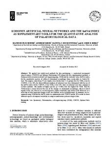
MLP is usually trained using an error back propagation algorithm. This popular algorithm works by iteratively changing a network’s interconnecting weights such that the overall error (i.e., between observed values and modeled network outputs) is minimized (Govindaraju and Rao 2000; Sudheer et al. 2002). Study Site and Relevant Data Khosrow Shirin watershed (approximately 610 km2 in area) from Fars Province in Iran between East longitudes (51°49´23" and 52°12´16") and North latitudes (30°37´02" and 30°59´34") was used as a case study catchment. The time series of precipitation data from four stations (Khosrow Shirin, Sedeh, Dehkade Sefid and Dozd Kord) was implemented for this study. The average daily precipitation on the watershed was calculated using Thissen polygon and used as input to the network. The time series of streamflow of Dehkade Sefid station (longitude 52°07´00", latitude 30°39´00") was used (see Figure 1). A 5-yr record (2002-2007) was selected. The 2002-2006 water years data (1460 daily values) were used for the training of MLPs and calibration of HMS SMA model. The 2006-2007 water year data was used for testing (365 daily values) of MLPs and validation of the calibrated HMS SMA model for this watershed. For comparison of the results of HMS SMA and MLPs the same calibration and validation periods for two methods were selected.

Figure2. Study site

Results and Discussion Most of the 12 parameters needed for the SMA algorithm (canopy interception storage, surface depression storage, maximum infiltration rate, maximum soil storage, tension zone storage, soil zone infiltration rate, and groundwater 1 percolation rate) were estimated through model calibration due to data scarcity of Khosrow Shirin watershed. This proved to be a very time-consuming process. A sensitivity analysis showed that groundwater percolation rate and Clark storage coefficient had the most effects on peak flows, and groundwater 2 percolation rate, surface depression storage capacity and impervious area had effects on annual flood volume. The calibration parameter constraints of HMS SMA model are shown below in Table 1. Four of the parameters (groundwater 1 and 2 storage depths and storage coefficients) were estimated by streamflow recession analysis of historic streamflow measurements (Linsley et al. (1958), Burnash et al. (1973), and Leavesley et al. (1983)). The groundwater 2 percolation rate was the other parameter estimated by model calibration. The recession curve is described by Table1. Calibration parameter constraints of HMS SMA Parameters Canopy Capacity (mm) Canopy Initial Storage Percentage (%) Clark Storage Coefficient (hr) Clark Time of Concentration (hr) Groundwater 1 Capacity (mm) Groundwater 1 Initial Storage Percentage (%) Groundwater 1 Percolation Rate (mm/hr) Groundwater 1 Storage Coefficient (hr) Groundwater 2 Capacity (mm) Groundwater 2 Initial Storage Percentage (%) Groundwater 2 Percolation Rate (mm/hr) Groundwater 2 Storage Coefficient (hr) Linear Reservoir GW 1 Coefficient (hr) Linear Reservoir GW 1 Steps () Linear Reservoir GW 2 Coefficient (hr) Linear Reservoir GW 2 Steps () Soil Capacity (mm) Soil Infiltration Rate (mm/hr) Soil Initial Storage Percentage (%) Soil Percolation Rate (mm/hr) Surface Capacity (mm) Surface Initial Storage Percentage (%) Tension Zone Capacity (mm)

Minimum 0.01 0.001 0.01 0 0.01 0.001 0.01 0.01 0.01 0.001 0.01 0.01 0 1 0 1 0.01 0.01 0.001 0.01 0.01 0.001 0.01

Maximum 1500 100 1000 1000 1500 100 500 10000 1500 100 500 10000 10000 100 10000 100 1500 500 100 500 1500 100 1500

Eq. (3), where qt = average daily flow at a future time with respect to the initial flow, qo; and Kr = recession constant. The time unit, t, is in days: qt = q o * K t r

(3)

Daily Outflow, (m3/sec)

To show the variation of recession constants, daily flows from 2/20/2005 to 8/20/2005 were observed (see Figure 3). From this graphic, the recession constants for the first (left) and second (right) parts of hydrograph and the mean value were calculated to be equal to 0.983, 0.993 and 0.988, respectively.

Time (day)

Figure3. Daily outflow hydrograph from 2/20/2005 to 8/20/2005 Based on field information summarized in Table 2 below, the slope of the watershed is equal to 13.8% (classified as moderate to gentle slopes), the value of 6.4 was selected as the initial value of the surface storage parameter. The final calibrated value of this parameter was equal to 10.0. Table2. Surface depression storage [Surface Storage Values from Bennett (1998)] Description Slope (%) Surface Storage (mm) Paved impervious areas NA 3.2-6.4 Steep, smooth slopes >30 1.0 Moderate to gentle slopes 5-30 6.4-12.7 Flat, furrowed land 0-5 50.8

In this study, the following combination of input data for precipitation and discharge was implemented for MLP training (see Table 3). For all of MLPs, three layer (5, 9 and 1) ANN models were trained using the Levenberg-Marquardt (LM) training algorithm. Also, the training of MLPs was performed by tangent sigmoid transfer functions. Table3. Combinations of MLPs

Model no.

Input combinations

1 2 3 4 5 6 7 8 9 10 11 12

P(t) P(t),P(t-1) P(t),Q(t-1) P(t),Q(t-1),Q(t-2) P(t),P(t-1),P(t-2),Q(t-1) P(t),P(t-1),P(t-2), P(t-3),Q(t-2) P(t),P(t-1),Q(t-1) P(t),P(t-1),Q(t-1),Q(t-2) P(t),P(t-1),Q(t-2) P(t),P(t-1),P(t-2),Q(t-1), Q(t-2) P(t),P(t-2),P(t-3),Q(t-1) P(t),P(t-2),P(t-3),P(t-4),Q(t-1) P = precipitation, Q= river flow, t = time

From the other study, it was concluded that MLP11 had the best prediction among the 12 input models. In this study, the number of neuron in the hidden layer changed and it led to higher prediction efficiency. Hence, in this study the prediction of HMS SMA model were compared just with MLP11 in the other study. The performance metrics of HMS SMA and MLP11 in terms of the root mean square error (RMSE) and coefficient of determination (R2) is shown in Figure 4. It can be seen that the values of RMSE at MLP11 are lower than for the HMS SMA model. The correlation between the observed flow and simulated flow via MLP11 was higher than for HMS SMA. The correlation values for MLP11 and HMS SMA models were equal to 0.90 and 0.84, respectively. The values of RMSE for MLP11 and HMS SMA models were 1.6 and 2.1 cubic meters per second (CMS), respectively. Clearly MLP11 performed better than HMS SMA and had a higher prediction efficiency. Plots of HMS SMA and MLP11 for flow forecasting for the validation period of 2006-2007 water years are also shown below (see Figures 5 and 6). Comparison of figures 5 and 6 attests this conclusion.

HMS SMA

MLP11

Figure4. Scatter plots of HMS SMA and MLP11 for the validation period

The observed and HMS SMA simulated monthly flood volumes for the validation period are shown in Figure 7. The same is shown in Figure 8 for MLP11. Comparison of these two figures shows that MLP11 can predict monthly and annual flood volumes better than can the HMS SMA model. The values of R2 for HMS SMA and MLP11 for annual flood volume prediction were equal to 0.86 and 0.93. The RMSE values for HMS SMA model and MLP11 for annual flood volume prediction were equal to 4.1 and 3.0 CMS. It should be noted that overestimation of HMS SMA was less than MLP11. This overestimation may be due to uncertainties about predictions by MLPs. Overall comparison of predictions from these two models indicates that MLP11 is a better method for continuous hydrologic modeling.

HMS SMA

Figure5. Plot of HMS SMA flow forecasting for the validation period

2006-7 Water Year, Validation Period

Figure5. Plot of RBF11 flow forecasting for the validation period Simulated

Figure6. Plot of MLP11 flow forecasting for the validation period

It should be noted that predictions by the HMS SMA model are also reliable. One of the weaknesses of HMS SMA is the additional efforts required for sensitivity analysis of results leading to longer time to perform the work.

HMS SMA

Figure7. Observed and HMS SMA Simulated monthly flood volume for the validation period

MLP11

Figure8. Observed and MLP11 Simulated monthly flood volume for the validation period

Conclusions HMS SMA and Multi Layer Perceptron network (MLP) are evaluated for predicting daily outflows at the outlet of Khosrow Shirin watershed, located in the north-west part of Fars Province in Iran. The results indicate that MLP can predict daily flow

with higher prediction efficiency than can HMS SMA. Comparison of annual flood volumes predicted by the two models also verifies the superiority of MLP. Application of MLP should be considered when there is not enough time and resources for sensitivity analysis and other procedures that are needed to be performed for HMS SMA applications. Also, MLP is much simpler to apply than HMS SMA and has fewer parameters. Therefore, it is concluded that MLP can be extended to continuous hydrologic modeling for watersheds with limited gages.

References ASCE Task Committee on Application of Artificial Neural Networks in Hydrology. (2000a). “Artificial neural networks in hydrology. I: Preliminary concepts.” J. Hydrol. Eng., 5(2), 115–123. Bennett, T. (1998). “Development and application of a continuous soil moisture accounting algorithm for the Hydrologic Engineering Center Hydrologic Modeling System (HEC-HMS).” MS thesis, Dept. of Civil and Environmental Engineering, Univ. of California, Davis, Beven, K. J. (2001). “Rainfall-Runoff Modelling.” The Primer. Wiley,Chichester, UK. Burnash, R. J. C., Ferral R. L., and McGuire, R. A. (1973). “A generalized streamflow simulation system: Conceptual modeling for digital computers.” United States Dept. of Commerce, National Weather Service, and State of California, Dept. of Water Resources, Sacramento, Calif. Dawson CW, Wilby R. (1998). “An artificial neural network approach to rainfallrunoff modeling.” Hydrological Sciences Journal 43(1): 47–66. Fleming, M., Neary, M. 2004. “Continuous Hydrologic Modeling Study with the Hydrologic Modeling System.” ASCE Journal of Hydrologic Engineering ,Volume 9, Issue 3, pp. 175-183. Govindaraju RS, Rao AR. (2000). “Artificial Neural Networks in Hydrology.” Kluwer Academic Publisher: Netherlands. Hydrologic Engineering Center (HEC). (2000). “Hydrologic modeling system HEC–HMS: Technical reference manual.” U.S. Army Corps of Engineers, Hydrologic Engineering Center, Davis, Calif. Kumar APS, Sudheer KP, Jain SK, Agarwal PK. (2005). “Rainfall-runoff modeling using artificial neural networks: comparison of network types.” Hydrological Processes 19: 1277–1291. Leavesley, G. H., Lichty, R. W., Troutman, B. M., and Saindon, L. G. (1983). “Precipitation-runoff modeling system: User’s manual.” United States Dept. of the Interior, Geological Survey, Denver.

Linsley, R. K., Kohler, M. A., and Paulhus, J. L. H. (1958). “Hydrology for engineers.” McGraw-Hill, New York. Maier HR, Dandy GC. (2000). “Neural networks for the prediction and forecasting of water resources variables: a review of modeling issues and applications.” Environmental Modeling and Software 15: 101–23. Mutlu. E, Chaubey. I, Hexmoor. H, Bajwa. S. G. (2008). “Comparison of artificial neural network models for hydrologic predictions at multiple gauging stations in an agricultural watershed.” Hydrological Processes Volume 22, Issue 26, Pages: 5097-

5106 Ponce, V. M. (1989). “Engineering hydrology.” Prentice-Hall, Englewood Cliffs, N.J. Sudheer, K. P., Gosain, A. K., and Ramasastri, K. S. (2002). “A data driven algorithm for constructing artificial neural network rainfall-runoff models.” Hydrology. Processes., 16(6), 1325–1330. Tokar AS, Johnson A. (1999). “Rainfall-runoff modeling using artificial neural networks.” Journal of Hydrologic Engineering, ASCE 4(3): 232–239. Tokar AS, Markus M. (2000). “Precipitation-runoff modeling using artificial neural networks and conceptual models.” Journal of Hydrologic Engineering, ASCE 5(2): 156–161.