Homing and navigation using one transponder P. Baccou, B. Jouvencel, V. Creuze
[email protected],
[email protected],
[email protected] LIRMM 161, rue Ada 34392 Montpellier cedex 5 France Abstract Homing and navigation capabilities are essential in many Autonomous Underwater Vehicle (AUV) applications. This paper presents the both problems with respect to a single beacon. The difficulties of this approach are due to the fact that a single range measurement does not completely constrain the beacon’s position in the vehicle frame. In order to triangulate his position, the AUV need to maneuver while measuring its displacements between ranges. In addition, range measurements are noisy and sometimes spurious, speed bias and underwater currents affect dead-reckoning measurements. Homing and navigation procedures are the same beginning. In a first time, we have an initialization phase which is necessary to obtain an initial estimate of the vehicle’s absolute position (the beacon absolute position is known onboard) and of the disturbances affecting the quality of the dead reckoned displacements (underwater components and speed bias). These initials estimates are refined during the actual displacement towards the beacon by means of a Kalman filter. Two kinds of navigation are used so as to maximize the information matrix and to maintain an accurate absolute position.
1. INTRODUCTION Many AUVs are currently operated in the world, either as prototypes or more recently with commercial purposes. The task consisting of locating the vehicle on the surface after completion of its mission is sometimes made difficult by sea state and lighting conditions. The vehicle is then generally fitted with one or several surface relocation systems (strobelight, radio beacon, radio transmission of the GPS position). In some cases, more sophisticated capabilities such as homing and docking are required. During under-ice operations, for instance, the AUV has to be able to return to the launch hole for recovery. APL with UARS [1] and Seashuttle [2], ISER with Theseus [3], and MIT with Odyssey [4] made under-ice experiments where the vehicle was fitted with an acoustic system providing the bearing angle of a beacon located near the launch hole. This measurement combined with the vehicle’s heading was used to steer the AUV towards the beacon. For the long term deployment of AUVs (Autonomous Ocean Sampling Network concept), the vehicles must be capable of returning to their moorings for recharging battery, data downloading and mission programming. Many different approaches have then been implemented and tested based on acoustic (Ultra Short Base Line, Short Base Line and Long Base Line
system), electromagnetic or optical sensors [4][5][6]. Long baseline navigation systems have also been used recently for the navigation of AUV [7][8][9][10]. Although, these systems can offer a good positioning accuracy, provided the array is correctly calibrated, they also have several drawbacks. The deployment and the recovery of the transponders as well as the calibration of the array are shiptime consuming and therefore expensive. Furthermore, the whole process has to be repeated each time the array move to a different place. The overall cost of the system is also substantial because of each beacon’s cost. Therefore, a different approach consisting of using a single beacon is being studied [11][12][13]. The advantage of such a solution is that the calibration reduces to the determination of the beacon’s location. Whereas the vehicle track is distorted by errors on the baseline calibration in the classical long baseline approach, any beacon position calibration error results in a shift of the AUV position equal to the calibration error in the single beacon approach. This approach could appear very attractive at first sight. It has, however, an important disadvantage associated with the fact that it is not possible to determine the vehicle’s position from a single ping. In classical long baseline navigation, the replies to a single ping can be used to triangulate the AUV’s position (provided the number of returns is sufficient and the measured ranges are valid). With a single beacon, the AUV has to ping the beacon from different places in order to triangulate its position. The baselines between ranges are then created by the displacements of the AUV, which have to be measured which maximal accuracy. As opposed to the solution presented in [13], which relies on an accurate dead reckoning system to measure the displacements, our concern is to provide a solution for vehicles equipped with low-cost sensors. The availability of a Doppler velocity log is then not an option due to the sensor’s cost, and we rather consider that the vehicle’s speed is approximately known by a priori calibration of the vehicle’s water speed as a function of propeller’s rpm. At this point, however, we consider that the vehicle has a reliable heading reference. The vehicle’s speed, used in the computation of the displacements, is then affected by a bias due to speed vs. rpm calibration errors and by the unknown underwater current components. These error sources will be estimated together with the vehicle’s position. Most of the time, the AUV know approximately its own initial absolute position even if it knows beacon’s absolute position. This is the case if the AUV has to dive deep after a surface GPS fix, or if it has traveled for a long time
underwater before getting within range of the beacon. For this reason, we will assume that the AUV has no knowledge of its initial absolute position. We separate our positioning algorithm in two steps, the first consisting to compute an initial estimate of the AUV’s absolute location and perturbations like underwater currents components and speed bias. The second step use a Kalman filter who permits to home the beacon or navigate in it area using information matrix. The paper is organized as follows: section II defines important reference frame. Section III describes the initialization procedure allowing to obtain the initial state estimate and its error covariance matrix used to initialize the Kalman filter. Section IV describes the Kalman filter in details and particularly how the vehicle’s motion between ping and reply is taken into account. Section V describes different heading command for homing or navigation thanks to improve the information matrix. Section VI presents simulation results.
2.
between ranges i and n can then be written: k =n k =n k =n i, n =∑Cθ k Cψ k uk ∆t −du∑Cθ k Cψ k ∆t +vcn∑∆t ∆ x k =i k =i k =i (2) k =n k =n k =n ∆yi,n =∑Cθ k Sψ k uk ∆t −du∑Cθ k Sψ k ∆t +vce∑∆t k =i k =i k =i
x0
dn Rm
d1
x
d2
dn-1
DEFINITIONS
R0
The location of the beacon in the local absolute reference frame R0 is (xb, yb, zb). This location can be known or not by the AUV, it depends on the mission, if we work in local reference, we use (0,0,zb) location. The axes x0 and y0 respectively point north and east, and z0 points down. The mobile frame Rm is located at the center of gravity of the vehicle with its axes xm, ym, zm parallel to x0, y0, z0. The knowledge of the beacon’s depth allows to convert the 3D problem into a 2D problem. The terminology ‘range’ in the remaining of the paper should then be understood as x-y range (slant range corrected for the depth difference between the vehicle and the beacon). The acoustic travel times are measured like in a Long Base Line system: the vehicle pings, the beacon replies upon reception after a given timeout and the vehicle detects the time of arrival of the reply. Slant ranges are calculated based on the known average speed of sound.
beacon
xb
yb
y
y0
Fig.1: Geometry of the initialization procedure Let Rm be the mobile frame at the time corresponding to the end of the rotation with the measure dn and (x,y) be the vehicle’s absolute position at that time. The ith range can be expressed as a function of the vehicle’s position at the end of the rotation and of the displacement between ranges i and n by:
[
di = (x b -x +∆x i,n ) +(yb -y+∆yi,n )
]
2 1/ 2
2
(3)
4 equations
3 holes
3. INITIALIZATION Criterion evolution
3.1. Principle
6 equations
The initialization of the beacon’s location consists of commanding a 360° rotation to the AUV while ranging to the beacon and measuring the displacements between pings (Fig.1). The vehicle would thus describe a circular path in the absence of underwater current or a distorted circle otherwise. In the presence of a speed bias (du) and of an underwater current (vcn,vce) all assumed to be constant, the north and east components of the vehicle’s displacement over a sampling period ∆t can be modeled by:
∆x=CθCψ(u −du)∆t +vcn∆t ∆y =CθSψ(u −du)∆t +vce∆t
Convergence hole
(1)
Where u is the vehicle’s calibrated water referenced speed,
θ is the pitch and ψ is the heading. The displacements
1 hole
Criterion evolution
Convergence hole
Fig.2 : Least square evolution of criterion The system of equations (3) can be solved for (x,y,du,vcn,vce) by non-linear least squares using the Levenberg-Marquardt algorithm. However, because the problem can have local minima, we could not initialize the search with (0,0,0,0,0) without risking convergence to an erroneous solution.
A study of least square criterion shows the instability of the solution. Figure 2 represents the minimal value of the least square criterion with respect to the location, the underwater current variation is comprised between +/- 2 m/s and the speed bias is not consider here. We can see that: • •
The number of equations increases the solution accuracy and a good convergence, The number of local minima decreases with respect to the number of equations.
Therefore, in order to initialize the algorithm closer to the correct solution, the system without current and speed bias is first solved starting at (x,y)=(0,0). The approximate vehicle position obtained in that case is then used to initiate the search in the presence of current (the current components and the bias being still initialized at 0).
3.2. Range pre-processing In our simulations, we chose to use a selection of 14 ranges for the estimation of (x,y,du,vcn,vce). Since ranges can sometimes be spurious because of noise or multi path, the 14 ranges have to be selected carefully. The set of ranges is first pre-filtered as follows: the difference between successive ranges is computed and a threshold is applied. If the difference is greater than the threshold, further testing is performed by looking at the ranges before and after the considered pair. Depending on the results of these additional tests, either both ranges are discarded or only one. A median method is then applied to the remaining ranges: • Select 14 ranges randomly (depends on the noise and on the number of ranges), • Compute the solution to equation (3), • Characterize the solution with the median of the range residuals. Repeat these steps N times and keep the set of 14 ranges providing the smallest median residual. N has to be chosen even larger that the range measurements are noisy. This is of course at the expense of a longer computation time. For the simulations, we used N=70 (it’s because of the greatest of the ranges noises: 20% are spurious and 20% are affected by a Gaussian noise). We can use N=30 for 10% of spurious ranges and 15% with a Gaussian noise but we increase the probability of erroneous solution.
(4)
Where d is the vector of the selected ranges, X=(x,y,vcn,vce,du)t, and ξ is a Gaussian noise on the measured ranges with variance matrix R. The non-linear least squares optimization provides the covariance matrix of X (Cramer-Rao lower bound):
(5)
the optimization is used to initialize the state vector of the Kalman filter described below, and the covariance matrix P is used to initialize the estimation error covariance matrix of the filter.
4. EXTENDED KALMAN FILTER 4.1. State equation The state vector is made up of the vehicle’s position (x,y) in R0, the vehicle’s depth (z), the components of the underwater current (vcn,vce) and the speed bias (du). The inputs are the vehicle’s heading ψ, its pitch θ and its waterreferenced speed u. The covariance matrix of the inputs is the diagonal matrix Cin =diag(σψ2,σθ2,σ u2 ) . The current and the speed bias are modeled as constant. The state noise vector is vk and its covariance matrix Qk. The state equation is then expressed by:
x x CθCψ (u −du )+vcn y y CθSψ (u −du )+vce z = z + −Sθ(u −du) ∆t +vk 0 vvcn vvcn ce ce 0 du du 0 k +1 k k
(6)
4.2. Observation equation The observation equation expresses the acoustic round-trip time of flight (T) as a function of the vehicle’s state at the time of the ping and at the time the vehicle receives the reply from the beacon. The vehicle’s motion between the ping and the reception is then taken into account, and observations are expressed in terms of all the state variables. The measurement noise on the travel times is represented by wk. It variance is Rk. The speed of sound is noted c and the beacon turn around time ∆tr.
{[
T = 1 (xb − xping ) +( yb − y ping ) +(zb − z ping ) c b
The system of equations (3) can be expressed by:
−1
Where H is the Jacobian of the ranges with respect to ψ, θ, u and Pe is the covariance matrix of ψ, θ, u. The result of
[(x −x
3.3. Uncertainty on the initial estimation
d = f(X,ψ,θ,u,∆t)+ξ
∂f(X) t −1 ∂f(X) ( P = HPe H t + R ) ∂X ∂X
recept
2
) +(yb− yrecept ) +(zb−zrecept ) ] 2
2
]+
2 1/ 2
2
2
1/ 2
}+∆t +w r
(7)
k
In general, a time of flight is buffered by the acoustic ranging system and made available for processing after a preset timeout following the ping time. The vehicle’s estimated state at that time is Xˆ k / k . The prediction step being applied first, the vehicle predicted state is Xˆ k +1/ k . Since the state prediction does not modify the current components and the speed bias estimates, these estimates are constant from the ping time to the time of flight processing
time. The vehicle’s position is then back propagated in time using the current state and the inputs, which were memorized since the ping. Since the ping time (tping) is known and the reception time (trecept) can be calculated by adding the time of flight to the ping time, the position of the vehicle at the ping and at the reception of the reply can then be calculated by:
[Cθi Cψi(ui −duk+1/k)+vcnk+1/k ]∆t xping=xk+1/k−i=∑ t ping t k +1/k yping=yk+1/k− ∑[Cθi Sψi(ui −duk+1/k)+vcek +1/k ]∆t i =t ping t k +1/k z ping=zk +1/k + ∑Sθi(ui −duk +1/k)∆∆ i =t ping t k +1/k xrecept=xk+1/k− ∑[Cθi Cψi(ui −duk+1/k)+vcnk +1/k ]∆t i =t recept yrecept=yk+1/k− t k +1/k[Cθi Sψi(ui −duk+1/k)+vcek +1/k ]∆t ∑ i =t recept t k +1/k zrecept=zk+1/k+ ∑Sθi(ui −duk+1/k)∆∆ i =t recept
(H
H kt +1 +D k +1C in D kt +1 +R +H k +1Sk +1 +S kt +1 H kt +1 (13)
When a time of flight is available, its validity is first checked by means of the Mahalanobis distance. The innovation and its variance are calculated by:
The filter equations are different from the classical equations in that inputs Uk=(ψ,θ,u)t can be found both in the state and the observation equations. Equations (6) and (7) can be rewritten: (9)
The filter proceeds in two steps. The first step is a prediction of the state based on the inputs in Uk. It basically corresponds to dead reckoning using the last estimates of the underwater current. The state is predicted together with its prediction error covariance Pk+1/k: (10)
The second step takes place when a time of flight is available. The predicted state is corrected based on the information carried by the new measurement. The prediction error covariance matrix Pk+1/k+1 is also computed:
The following Jacobian matrices have to be calculated:
P
k +1 k +1/k
)
4.4. Time of flight validation
4.3. Equations of the filter
X k +1/ k +1= X k +1/ k + Kk +1(Z k +1−h(X k +1/ k ,U k )) Pk +1/ k +1= Pk +1/ k − Kk +1(H k +1Pk +1/ k + S t ) k +1
(
K k +1 = Pk +1/k H kt +1 +S k +1
(8)
Xk +1/k =f(Xk/k,Uk) Pk +1/k =Fk Pk/k Ft +J kCin J t +Qk k k
(12)
Sk+1 = Jk+1CinDtk+1 is a correlation term accounting for the fact that inputs are both in the state and the observation equations. Because of this correlation, the expression of the Kalman gain is a little more complicated than usual:
t k +1/k
X k +1=f(Xk,Uk)+ vk Zk =h(Xk,U k)+ w k
∂f(X,U) ∂f(X,U) Jk = ∂X XU=XUk/k , ∂U XU= XUk/k , ∂h(X,U) ∂h(X,U) Hk +1= Dk +1= ∂U XU =XUk +1/k ∂X XU=XUk +1/k 1 , 1 , Fk =
(11)
ν k +1=Tk +1−h(Xk +1/k,Uk +1)
(14)
Pν k +1 = H k +1 Pk +1/k H kt +1 + D k +1C in D kt +1 + R
(15) + H k +1S k +1 + S kt +1 H kt +1 The time of flight Tk+1 is validated and used to correct the predicted state if it passes the following test: ν kt +1 Pυ−k1+1 ν k +1 < γ 2
with γ2 typically equal to 3.
(16)
5. VEHICLE NAVIGATION A study of the information matrix similar to that described in [14] has showed that the trajectory that maximizes the information (or conversely minimize the estimation error covariance) consists of leaving the beacon on either side of the vehicle so that the vehicle’s heading deviates by 90° from the line joining the vehicle and the beacon (the vehicle describes a circle centered at the beacon). In order to increase the information, we use the following procedure. At the end of the 360° rotation, the vehicle is commanded to move at 90° with respect to the beacon. When this condition is achieved, the volume of the prediction error covariance ellipsoid is calculated by: C 0 = det(P)
(17)
When a new time of flight is made available and used by the filter, the volume is calculated for the new covariance matrix: C k = det(Pk/k )
(18)
The homing is not satisfying since the vehicle never
)
−1
reaches the beacon. Going straight to the beacon is, however, neither a desired configuration because the range measurements cannot correct efficiently lateral errors along the vehicle track, so that the vehicle could actually miss the beacon. In the case of speed bias is considered, the heading command law described in [12] do not satisfied the speed convergence even if we change the speed of the vehicle during homing. We notice that the deviation arrived quickly to 56°. We introduced the distance to the beacon (“range”) in the deviation angle: C k π (19) ψ k = ψ b k + 1 − exp k * range * 2 C k − C 0 Where k is a speed homing coefficient. It’s very difficult for the filter to converge to the real speed bias when heading is changing all the time (the speed bias is considered on the longitudinal vehicle axis). For this reason, we keep the same direction during some measurements before compute the new heading. The case of navigation is simplest, the vehicle keeps circling around the beacon until the ration of Ck over C0 is smaller that a preset threshold (function of N). The AUV then reaches its first waypoint and starts doing its survey. At this point the vehicle still uses the filter to estimate its position during the survey.
6. SIMULATION RESULTS The algorithm described above has been tested in simulation using the simulator of the torpedo-shaped AUV Taipan developed at LIRMM [15]. In the homing simulation, the current was set so as to have a 0.2 m/s magnitude and a 60° direction. The speed bias was set at 0.2 m/s. In order to simplify the visualization of the tracks, the absolute position of the beacon is subtracted from all the absolute positions. The beacon then appears to be located at (0,0) on the plots. During the initialization phase, the vehicle dead-reckons its displacements between ranges without any knowledge of its absolute initial position. For the plots, however, the deadreckoned position was initialized by the vehicle’s actual initial position. After the initialization, the filter provides the estimated position of the vehicle in R0, which is used to steer the AUV so as to leave the beacon at 90°. We present results for homing and two different vehicle tracks. The first track consists of homing (Fig.3). The second track consists of parallel legs (Fig.4) with a current of 0.14m/s magnitude and 197° direction, the speed bias is 0.19m/s . The third track consists of radial legs (Fig.5) with a current of 0.11m/s magnitude and 72° direction, the speed bias is 0.15m/s.
Fig.3 : homing trajectory (dark: estimated, light: actual) and perturbations results Throughout the simulation, the ranges (or times of flight) were simulated so that 20% of them would be spurious, 20% would be affected by a Gaussian noise with a 10m standard deviation, and the remaining would be affected by a Gaussian noise with an 0.5m standard deviation. When you realize homing, the difficulty is to reduce the distance without deteriorate filter solutions. In figure 3, we can see the difficult speed bias convergence. This convergence is more precise when you bring nearer to the beacon. We think that this is the fact to dead-reckoned and distance are in the same order. The AUV starts its 360° rotation at the square mark located at about (-200,-200) with an initial heading of about 135°. The dead-reckoned path is a circle (dark line) since the vehicle is not aware of the current. The actual vehicle trajectory is show by the distorted circle (light line).
Fig.4 : Parallel trajectory (dark: estimated, light: actual) and perturbations results
Fig.5 : Radial trajectory (dark: estimated, light: actual) and perturbations results The estimated position of the vehicle at the end of the initialization is shown by a cross at about (-200,-150) in figure 4. It can be seen that this estimated position is very close to the actual position of the vehicle after the distorted circle. The estimated position then jumps from the end of the
circle to these coordinates. From there, the actual and estimated trajectories are very close to each other and remain so until the end. The estimates of the underwater current and speed bias components along the runs are shown in figure 4 and 5 (the straight lines show the actual current and speed bias components). It can be seen that the estimates converge to the correct values during the 90° navigation phase. The radial track gives better results principally because of the vehicle travels at varying headings and during different straight line.
7. CONCLUSION In addition to its interest as an alternate solution to classical long baseline, we believe that the range-only solution is worth studying in the more general framework of multiple vehicle operations. Navigation with respect to a beacon by range measurements supposes that the vehicle is able to estimate its position relative to the beacon. If the beacon becomes mobile (carried by another AUV), then the AUV could be able to determine its relative position exactly in the same way, provided that the beacon can transmit its depth and displacements to the AUV by acoustic communications. Assuming clock synchronization between multiple AUVs, it is then possible to consider having a master vehicle that would ping and transmit its displacements and have the other AUVs determine their position relative to the master AUV. The simulation results presented in this paper were obtained using the simulator of the Taipan AUV developed at LIRMM (Fig.6). An acoustic modem incorporating a range measurement capability to a beacon has recently been integrated in Taipan, with the objective of experimenting the algorithm. In addition to the modem, the vehicle is fitted with a pressure sensor, pitch rate and yaw rate gyrometers, a DGPS, a magnetic compass, a pitch and roll inclinometer. The vehicle speed is based on a priori propeller rpm / speed calibration, so that estimation of the underwater current is critical. Other future works concerns movement generation and docking.
Fig.6 : Taipan with the acoustic modem transducer (length: 1.8m, diameter: 15 cm, weight: 30 kg)
REFERENCES [1] R.E. Francois et al, “Unmanned Arctic research submersible (UARS) system development and test report,” Technical Report, n° APL-UW 7219, Applied Physics Laboratory, University of Washington, 1972. [2] J. Osse et Russell Ligh, “Line deployment by a miniature AUV under Arctic ice,” [3] B. Butler, “Field trials of the Theseus AUV,” 9th
Unmanned Untethered Submersible Technology, Durham NH, 25-27 septembre 1995. [4] J.G. Bellingham et al, “AUV operations in the Arctic,” Sea Ice Mechanics and Arctic Modeling Workshop proceedings, Anchorage, Alaska, USA, April 25-28, 1995. [5] D.R . Yoerger et al , “ System testing of the Autonomous Benthic Explorer,” IARP’94 workshop, Monterey, 1994. [6] S. Cowen et al, “Underwater docking of autonomous undersea vehicles using optical terminal guidance,” MTS/IEEE Oceans’97, Halifax, 6-9 Octobre 1997. [7] J.G. Bellingham, T.R. Consi, U. Tedrow and D. Di Massa, “Hyperbolic acoustic navigation for underwater vehicles: implementation and demonstration”, Proceedings of the 1992 symposium on Autonomous Underwater Vehicle Technology, June 2-3, Washington, DC, USA. [8] D.K. Atwood, J.J. Leonard, J.G. Bellingham, and B. A. Moran, “An acoustic navigation system for multiple vehicles”, 9th Int. Symp. on Unmanned Untethered Submersible Technology, pp.202-208, New Hampshire, September 25-27, 1995. [9] J. Vaganay, J.G. Bellingham and J.J. Leonard, “Comparison of fix computation and filtering for autonomous acoustic navigation”, International Journal of Systems Science, vol.29, n°10, pp. 1111-1122, 1998. [10] A. Matos, N. Cruz, A. Martins and F.L. Pereira, “Development and implementation of low-cost LBL navigation system for an AUV”, OCEANS ‘99 MTS/IEEE. Riding the Crest into the 21st Century, volume 2, pages 774-779. [11] A.P. Scherbatyuk, “The AUV positioning using ranges from one transponder LBL”, OCEANS ’95 MTS/IEEE. Challenges of Our changing Global Environment. Conference Proceedings., Volume 3, pages 1620-1623 [12] J.Vaganay, P. Baccou, B. Jouvencel, “Homing by acoustic ranging to a single beacon”, OCEANS ’00 MTS/IEEE, Conference and Exhibition, Proceedings Volume 2, pages 1457-1462, September 11-14, Providence, RI, 2000. [13] M.B. Larsen, “Synthetic long baseline navigation of underwater vehicles”, OCEANS ‘00 MTS/IEEE, Conference and Exhibition, Proceedings Volume 3, pages 2043-2050, September 11-14, Providence, RI, 2000. [14] J. S. Feder, J. J. Leonard, C. M. Smith, “Adaptive mobile robot navigation and mapping,” Int. Journal of Robotics Research, Special Issue on Field and Service Robotics, July 1999. [15] J.Vaganay, B. Jouvencel, P. Lepinay, R. Zapata, “An AUV for very shallow water applications”, World Automation Congress, Anchorage, Alaska, USA, May 10-14, 1998.