Using Many Cameras as One Robert Pless Department of Computer Science and Engineering Washington University in St. Louis, Box 1045, One Brookings Ave, St. Louis, MO, 63130
[email protected]
Abstract We illustrate how to consider a network of cameras as a single generalized camera in a framework proposed by Nayar [13]. We derive the discrete structure from motion equations for generalized cameras, and illustrate the corollaries to the epi-polar geometry. This formal mechanism allows one to use a network of cameras as if they were a single imaging device, even when they do not share a common center of projection. Furthermore, an analysis of structure from motion algorithms for this imaging model gives constraints on the optimal design of panoramic imaging systems constructed from multiple cameras.
1
Figure 1. A schematic of a multi-camera system for an
Introduction
autonomous vehicle, including a forward facing stereo pair, two cameras facing towards the rear, and a panoramic multicamera cluster in the middle. The lines represent the rays of light sampled by these cameras. This paper presents tools for motion analysis in which this entire system is viewed as a single camera in the generalized imaging framework [13].
Using a set of images to solve for the structure of the scene and the motion of the camera has been a classical problem in Computer Vision for many years. For standard pinhole cameras this is fundamentally a difficult problem. There are strictly ambiguous scenes — for which it is impossible to determine all parameters of the motion or the scene structure [1]. There are also effectively ambiguous scenes, for which the structure from motion solution is illconditioned and small errors in image measurements can lead to potentially large errors in estimating the motion parameters [8, 21]. These limitations have led to the development of new imaging geometries. Panoramic and omni-directional sensors with a single center of projection (e.g. [15]) have many direct corollaries to the pinhole camera model, including an epi-polar geometry [24], a variant of the Fundamental Matrix [10] and ego-motion constraints [12, 6]. The larger field of view gives advantages for ego-motion estimation [5, 16]. Non-central projection cameras allow for greater freedom in system design because they eliminate the technically challenging task of constructing a system of cameras which share a nodal point. One example of a multi-camera
network where the cameras do not share a nodal point is illustrated in 1. Specific multi-camera and catadioptic camera designs have been introduced with an analysis of their imaging geometry, calibration [11, 20, 14, 4], and the constraints relating the 3D scene structure and the relative camera positions or motions [9, 7, 23]. Many natural camera systems, including catadioptric systems made with conical mirrors and incorrectly aligned lenses in standard cameras, have a set of viewpoints well characterized by a caustic [25]. A further generalization of the allowable camera geometry is the oblique camera model [17] that applies to imaging geometries where each point in the environment is imaged at most once. A similar formulation gives design constraints on what camera geometries result in stereo systems with horizontal epi-polar 1
A raxel defines how a pixel samples the scene. This sampling is assumed to be centered around a ray starting at a point X,Y,Z, with a direction parameterized by (φ, θ). This pixel captures light from a cone around that ray, whose aspect ratio and orientation is given by (fa , fb , Υ). The light intensity captured may also be attenuated, these radiometric quantities may differ for every pixel. For the geometric analysis of multiple images, we simplify this calibration so that it only includes the definition of the ray that the pixel samples. This gives a simpler calibration problem which requires determining, for each pixel, the Pl¨ucker vectors of the sampled line. Since Pl¨ucker vectors are required for the mathematical analysis presented later, the following section gives a brief introduction.
Figure 2. (Top) The generalized imaging model [13] expresses how each pixel samples the light-field. This sampling is assumed to be centered around a ray starting at a point X,Y,Z, with a direction parameterized by (φ, θ), relative to a coordinate system attached to the camera. The simplified model captures only the direction of the ray, parameterized by its Pl¨ucker vectors q, q 0 .
2.2
In order to describe the line in space that each pixel samples in this more general camera setting, we need a mechanism to describe arbitrary lines in space. There are many parameterizations of lines, but Pl¨ucker vectors [18] give a convenient mechanism for the types of transformations that are required. The Pl¨ucker vectors of a line are a pair of 3vectors: q, q 0 , named the direction vector and moment vector. q is a vector of any length in the direction of the line. Then, q 0 = q × P , for any point P on the line. There are two constraints that this pair of vectors must satisfy. First, q · q 0 = 0, and second, the remaining five parameters are homogeneous, their overall scale does not affect which line they describe. It is often convenient to force the direction vector to be a unit vector, which defines a scale for the homogeneous parameters. The set of all points that lie on a line with these Pl¨ucker vectors is given by:
lines [19]. The “generalized camera model” [13] is briefly introduced in Section 2.1, and encompasses the imaging geometry of all the camera designs discussed above. The main contribution of this paper is to express a multi-camera system in this framework and then to derive the structure from motion constraint equations for this model. The differential structure from motion constraints give an error function which defines a minimization problem for motion estimation (summarized in Section 3). Considering the Fisher Information Matrix of this error function makes it possible to give quantitative comparisons of different camera designs in terms of their ability to estimate ego-motion (Section 4).
2 2.1
¨ Plucker Vectors
(q × q 0 ) + αq, ∀α ∈ R.
(1)
If q is a unit vector, the point (q × q 0 ) is the point on the line closest to the origin and α is the (signed) distance from that point.
Background Generalized Camera Model
2.3 The generalized camera model was introduced as a tool to unify the analysis and description of the widely diverging sets of new camera designs. This model abstracts away from exactly what path light takes as it passes through the lenses and mirrors of an arbitrary imaging system. Instead, it identifies each pixel with the region of space that affects that sensor. A reasonable model of this region of space is a cone emanating from some point. A complete definition of the imaging model has been defined in terms of “raxels” [13], (see Figure 2). An image taken by a generalized camera is defined as the set of raxel measurements captured by the system.
¨ Plucker Vectors of a Multi-Camera System
A pinhole camera whose nodal point is at the origin samples a pencil of rays incident on the origin. If the calibration matrix K maps image coordinates to coordinates on the normalized image plane, a pixel (x, y) samples along a ray with Pl¨ucker vector hKhx, y, 1i> , 0i. The moment vector of the Plucker ray is zero because the point (0, 0, 0) is on the ray. A camera not at the origin has an internal calibration matrix K, and a rotation R, and a translation T which transform points from the camera coordinate system to the fiducial coordinate system. In this case, the ray sampled by a particular pixel on the camera a direction vector q = 2
RKhx, y, 1i> , and a moment vector q × T . The imaging geometry of the entire multi-camera system is represented simply by the collective list of the rays sampled by the individual cameras. For a single camera, a differential motion on the image plane defines a differential change in the direction of the sampled ray. For a camera not centered at the origin, the differential change in the direction vector is: ∂q(x,y) = RKhdx, 0, 0i> , and ∂q(x,y) = RKh0, dy, 0i> . dx dy The differential change in the moment vector is: 0
∂q 0 (x,y) dx >
q2 · (Rq10 + R(T × q1 )) + q20 Rq1 = 0. This completely defines how two views of a point constrain the discrete motion of a generalized camera. Using the convention that [T ]x is the skew symmetric matrix such that [T ]x v = T × v for any vector v, we can write: Generalized Epi-polar Constraint T
q2 T Rq10 + q2T R[T ]x q1 + q20 Rq1 = 0.
=
(x,y) RKhdx, 0, 0i> × T , and ∂q dy = RKh0, dy, 0i × T . In Section 3.2, this will be used to define the relationship between optic flow measurements in each camera and the motion of the entire system. We proceed first, however, with the constraints relating discrete motions of the camera system to the image captured by each camera.
3
For standard perspective projection cameras, q10 = q20 = 0, and what remains: q2T R[T ]x q1 = 0, is the classical epipolar constraint defined by the Essential matrix. Strictly speaking, this is not exactly analogous to the epi-polar constraint for standard cameras. For a given point in one image, the above equation may have none, one, several, or an infinite number of solutions depending on what the exact camera geometry is. The name generalized epi-polar constraint, however, is fitting because it describes how two corresponding points constrain the relative camera motions. Given the camera transformation R, T and corresponding points, it is possible to determine the 3D coordinates of the world point in view. Using Equation 1, and transforming the first line into the second coordinate system, solving for the position of the point in space amounts to finding the intersection of the corresponding rays. This requires solving for the parameters α1 , α2 , which is the corollary of the depth in typical cameras:
Motion Estimation
This section presents the structure from motion constraint equations for generalized cameras. We present first the discrete motion equations — how a pair of corresponding points constrain the rotation and translation between camera viewpoints. Then we present the differential motion constraints relating continuous camera motions to optic flow.
3.1
Discrete Motion
R((q1 × q10 ) + α1 q1 ) + T = (q2 × q20 ) + α2 q2
Suppose, in two generalized images, we have a correspondence between pixel (x1 , y1 ) in the first image and pixel (x2 , y2 ) in a second image. This correspondence implies that the rays sampled by these pixels (hq1 , q1 0 i, and hq2 , q2 0 i) must intersect in space. When the camera system undergoes a discrete motion, the fiducial coordinate systems are related by an arbitrary rigid transformation. There is a rotation R and a translation T which takes points in the first coordinate system and transforms them into the new coordinate system. After this rigid transformation, the Pl¨ucker vectors of the first line in the second coordinate system become: hRq1 , Rq10 + R(T × q1 )i .
Collecting terms leads to the following vector equation whose solution allows the reconstruction of the 3D scene point P in the fiducial coordinate system: Generalized Point Reconstruction α1 Rq1 − α2 q2 = (q2 × q20 ) − R(q1 × q10 ) − T, solve above equation for α1 , and use below P = q1 × q10 + α1 q1
3.2
Continuous Motion
In the differential case, we will consider the image of a point P in space which is moving (relative to origin of the camera coordinate system) with a translation velocity ~t, and an angular velocity ω ~ . The instantaneous velocity of the 3D point is: P˙ = ω ~ × P + ~t.
(2)
A pair of lines with Pl¨ucker vectors hqa , qa 0 i, and hqb , qb 0 i intersect if and only if: qb · qa0 + qb0 · qa = 0.
(4)
(3)
For a point in space to lie on a line with Pl¨ucker vectors hq, q 0 i, the following must hold true:
This allows us to write down the constraint given by the correspondence of a point between two images, combining Equations 2 and 3
P × q − q 0 = ~0; 3
As the point moves, the Pl¨ucker vectors of the lines incident upon that point change. Together, the motion of the point and the change in the Pl¨ucker vectors of the line incident on that point must obey:
Generalized Optic Flow Equation q˙ = ω ~ ×q+
∂ (P × q − q 0 ) = ~0, or, dt P˙ × q + P × q˙ − q˙0 = 0
−(~t × q) × q + q˙0 × q − (~ ω · q)q 0 α
(9)
For standard perspective projection cameras, q 0 = 0, and q˙ = 0, and this simplifies to the standard optic flow equation (for spherical cameras): 0
In terms of the parameters of motion, this gives: (~ ω × P + ~t) × q + P × q˙ − q˙0 = ~0. (~ ω × P + ~t) × q = q˙0 − P × q. ˙
q˙ = −(~ ω × q) − (5)
One approach to finding the camera motion starts by finding an expression relating the optic flow to the motion parameters that is independent of the depth of the point. This differential form of the epi-polar constraint is:
which are constraints relating the camera motion and the line coordinates incident on a point in 3D for a particular rigid motion. On the image plane, the image of this point is undergoing a motion characterized by its optic flow (u, v). In Section 2.3, we related how moving across an image changes the rays that are sampled. This allows us to write how the coordinates of the Pl¨ucker vectors incident on a point in 3D must be changing: ∂q ∂q u+ v, ∂x ∂y ∂q 0 ∂q 0 q˙0 = u+ v, ∂x ∂y
(~t × q) × q α
q˙ × ((~t × q) × q) = −(~ ω × q) × ((~t × q) × q). This same process can be applied to generalized cameras, giving:
q˙ =
Generalized Differential Epi-polar Constraint (6)
(q˙ + ω ~ × q) × ((~t × q) × q − q˙0 × q + (~ ω · q)q 0 ) = 0, (10)
so that we can consider q˙ and q˙0 to be image measurements. Then we can substitute Equation 1 into Equation 5 to get:
which, like the formulation for planar and spherical cameras, is bilinear in the translation and the rotation and independent of the depth of the point. The next section introduces a tool to calculate the sensitivity to noise of this constraint for any specific camera model.
(~ ω × ((q × q 0 ) + αq) + ~t) × q = q˙0 − ((q × q 0 ) + αq) × q. ˙ or, (~ ω ×(q×q 0 ))×q+α(~ ω ×q)×q+~t×q = q˙0 −(q×q 0 )×q−αq× ˙ q. ˙ (7) The following identities hold when |q| = 1, 0
3.3
Fisher Information Matrix
Let p~ be a vector of unknowns, (in our problem, h~t, ω ~ , α1 , . . . αn i), and Z be the set of all measurements (in our case the u, v that are used to calculate q, ˙ q˙0 using equation 6). The Fisher Information Matrix, F , is defined to be [22]1 :
0
(~ ω × (q × q )) × q = (~ ω · q)(q × q ), and, (~ ω × q) × q) = (~ ω · q)q − ω ~, 0 0 (q × q ) × q˙ = −(q · q)q, ˙ Simplifying Equation 7 and collecting terms gives: 0
0
>
F = E[
0
α((~ ω ·q)q −~ ω +q × q)+ ˙ ~t×q = q˙ +(q · q)q ˙ −(~ ω ·q)(q ×q ) (8) This vector equation can be simplified by taking the cross product of each side with the vector q, which gives:
∂ ln p(Z|p) ∂ ln p(Z|p) ]. ∂p ∂p
For any unbiased estimator of the parameter p, the Cramer-Rao inequality guarantees that the covariance maˆ )(p − p ˆ )> ]), is at least as trix of the estimator, (E[(p − p great as the inverse of the Fisher information matrix:
−α(~ ω × q) + (~t × q) × q = q˙0 × q − (~ ω · q)q 0 − αq. ˙ Collecting the terms that relate to the distance of the point along the sampled ray, then dividing by α gives:
ˆ )(p − p ˆ )> ] ≥ F −1 . E[(p − p
−(~t × q) × q + q˙0 × q − (~ ω · q)q 0 α which can be written more cleanly to define the optic flow for a generalized camera under differential motion:
If we model the probability density function of errors in the motion field measurements as Gaussian distributed,
(−~ ω × q + q) ˙ =
1 This presentation follows [8] and [21], which use the Fisher Information Matrix to study ambiguities and uncertainties for motion estimation with standard cameras.
4
zero mean, and covariance σ 2 I, then the Fisher Information matrix can be written: F(~t,~ω,α1 ,...αn )
4 Analysis Different visual system designs are appropriate for different environments. Within the context of estimating egomotion, the relevant parameters are the system motion and the distances to points in the scene. The environment is defined as the distribution of these parameters that the system will experience. This is a distribution over the set of parameters (~t, ω ~ , α1 , . . . αn ). In our simulation, we choose this distribution D as follows:
1 X ∂hi > ∂hi = 2 , σ i=1...n ∂p ∂p
where hi is the function that defines the exact optic flow at pixel i for a particular set of motion parameters and scene depths (these subscripts are to remind the reader that F is dependent on the these particular parameters). To determine the form of hi , we start with the generalized optic flow equation:
• ~t chosen uniformly such that |~t| < 1. • ω ~ chosen uniformly such that |~ ω | < 0.01.
−(~t × q) × q + q˙0 × q − (~ ω · q)q 0 q˙ = ω ~ ×q+ α
•
1 αi
chosen uniformly such that 0 ≤
1 αi
≤ 1.
Each point in this distribution has an associated Fisher Information Matrix, the (randomized, numerical) integration of this matrix over many samples from this distribution is a measure of the fitness of this camera system in this environment: X FD = F(~t,~ω,α1 ,...αn )
and multiply through by the α and re-arrange terms to get: q˙0 × q − αq˙ = −α~ ω × q + (~t × q) × q + (~ ω · q)q 0 Equation 6 defines how moving on the image plane changes the Pl¨ucker coordinates of the ray being sampled. Define A and B to be the pair of 2 × 3 Jacobians relating motion on the image to changes in the direction of sampled ray such that:
(~ t,~ ω ,α1 ,...αn )∈D
Figure 3 displays FD for a number of different camera designs. Each of these situations merits a brief discussion: 1. A standard video camera with a 50◦ field of view. The covariances reflect the well known ambiguities between some translations and rotations.
q˙ = ~uA, q˙0 = ~uB, where ~u =< u, v > is the optic flow measured on the image. Then we can rewrite the generalized optic flow equation as: ~uB[q] − α~uA = −α~ ω × q + (~t × q) × q + (~ ω · q)q 0 , or ~u(B[q] − αA) = −α~ ω × q + (~t × q) × q + (~ ω · q)q 0 (11)
2. The flow fields from a stereo pair have the same ambiguities as a single camera. The covariance matrix has a larger magnitude because two cameras capture twice the amount of data. This matrix (and these ambiguities) do not apply to algorithms which use correspondence between the stereo imagery as part of the motion estimation process. 3. A “stereo” camera pair in which one camera looks backwards does not have the standard rotationtranslation ambiguity, but has a new confusion between rotation around the axis connecting the cameras and rotation around the common viewing axis of the cameras.
Defining C = (B[q] − αA)> ((B[q] − αA)(B[q] − αA)> )−1 , we can then isolate the optic flow and get the terms we need to define the Fisher Information Matrix2 : hi = ~u = (α~ ω × q + (~t × q) × q − (~ ω · q)q 0 )C.
4. A camera system with cameras facing in opposite directions but aligned along their optic axis is perhaps the best design for two standard cameras. The “line” ambiguity (discussed under camera design 1) is still present
It is thus possible to create an analytic form giving the Fisher Information Matrix for a particular environment (camera motion and scene structure). In the following section we use this to measure of how well a particular vision system can measure its ego-motion in a variety of environments.
5. Three cameras aligned along three coordinate axes show a small covariance between translation and rotation. This may be an artifact of the strong covariances between each camera pair.
2 Recall that the matrices A, B, C, and the Plucker vectors q, q 0 are different at each pixel, we have dropped the subscripts to facilitate the derivations
5
6. Six cameras placed to view in opposite directions along coordinate axes show no ambiguities. 7. Six cameras placed to view in every direction, but not as matched pairs along each viewing axis. This situation models the “Argus Eye” system [3], which reported very accurate estimates of system rotation, again arguing that the covariance shown here may be (1) an artifact of the strong covariance (in rotation) between each camera pair. These results fit published empirical data which finds that system rotation and translation is much better constrained for a multi-camera system (the Argus Eye), than (2) for single cameras [3, 2] (see Figure 4). In this work we have carried out an analytic comparision of different types of cameras (as opposed to different algorithms) for the ego-motion estimation problem. As technology and computational power increase, the effectiveness (3) of visual algorithms will be limited only by inherent statistical uncertainties in the problems they are solving. The Fisher Information Matrix is a powerful analysis technique that can apply to any problem which involves searching for a parameter set that minimizes an error function. Design- (4) ing camera systems optimized for particular environments is necessary to make computer vision algorithms successful in real world applications.
References
(5)
[1] G. Adiv. Inherent ambiguities in recovering 3-D motion and structure from a noisy flow field. IEEE Transactions on Pattern Analysis and Machine Intelligence, 11:477–489, 1989. [2] Patrick Baker, Cornelia Fermuller, Yiannis Aloimonos, and Robert Pless. A spherical eye from multiple camera (makes better models of the world). In Proc. IEEE Conference on Computer Vision and Pattern Recognition, 2001. [3] Patrick Baker, Robert Pless, Cornelia Fermuller, and Yiannis Aloimonos. New eyes for shape and motion estimation. In Biologically Motivated Computer Vision (BMCV2000), 2000.
(6)
(7) Figure 3. The FD matrix for a variety of different camera forms. Shown is the 6 × 6 sub-matrix indicating covariance between the translation and rotational parameters. This matrix is symmetric, and the rows correspond, in order, to: ωx , ωy , ωz , tx , ty , tz . Outlined are covariances indicating a potential uncertainty or ambiguity between different motion parameters. See discussion in the text.
[4] Simon Baker and Shree K. Nayar. A theory of singleviewpoint catadioptric image formation. International Journal of Computer Vision, 1999. [5] T Brodsk´y, C Ferm¨uller, and Y Aloimonos. Directions of motion fields are hardly ever ambiguous. International Journal of Computer Vision, 26:5–24, 1998. [6] Atsushi Chaen, Kazumasa Yamamzawa, Naokazu Yokoya, and Haruo Takemura. Acquisition of three-dimensional information using omnidirectional stereo vision. In Asian Conference on Computer Vision, volume I, pages 288–295, 1998. [7] P. Chang and M. Hebert. Omni-directional structure from motion. In Proc. IEEE Workshop on Omnidirectional Vision, pages 127–133, Hilton Head Island, SC, June 2000. IEEE Computer Society.
6
[17] Tomas Pajdla. Stereo with oblique cameras. International Journal of Computer Vision, 47(1):161–170, 2002. [18] J. Pl¨ucker. On a new geometry of space. Philisophical Transactions of the Royal Society of London, 155:725–791, 1865. [19] Steven M Seitz. The space of all stereo images. In Proc. International Conference on Computer Vision, volume I, pages 26–33, 2001.
Figure 4. (Middle) The Argus eye system [3] was con-
[20] H Y Shum, A Kalai, and S M Seitz. Omnivergent stereo. In Proc. International Conference on Computer Vision, pages 22–29, 1999.
structed as a system of cameras, but can also be modelled as a single non-central projection imaging system. Empirical studies demonstrate that ego-motion estimation is better constrained for the Argus system than a single camera [2]. (Left) A sphere represents the set of all possible translation directions. Each point is colored by the error in fitting image measurements to that translation direction (darker is higher error). For a single camera, this error surface has an extended minimum region, indicative of the difficulty in determining the exact translation. (Right) Using all cameras simultaneously, the best translation direction is very well constrained.
[21] S. Soatto and R. Brockett. Optimal structure from motion: Local ambiguities and global estimates. In CVPR, 1998. [22] H W Sorenson. Paramerer Estimation, Principles and Problems. Marcel Dekker, New York and Basel, 1980. [23] Peter Sturm. Mixing catadioptric and perspective cameras. In Proc. of the IEEE Workshop on Omnidirectional Vision, 2002. [24] T Svoboda, T Pajdla, and V Hlavac. Epipolar geometry for panoramic cameras. In Proc. European Conference on Computer Vision, 1998. [25] Rahul Swaminathan, Michael Grossberg, and Shree Nayar. Caustics of catadioptric cameras. In Proc. International Conference on Computer Vision, 2001.
[8] K. Daniilidis and M. E. Spetsakis. Understanding noise sensitivity in structure from motion. In Y. Aloimonos, editor, Visual Navigation: From Biological Systems to Unmanned Ground Vehicles, chapter 4. Lawrence Erlbaum Associates, Mahwah, NJ, 1997. [9] Christopher Geyer and Kostas Daniilidis. Structure and motion from uncalibrated catadioptric views. In Proc. IEEE Conference on Computer Vision and Pattern Recognition, 2001. [10] Christopher Geyer and Kostas Daniilidis. Properties of the catadioptric fundamental matrix. In Proc. European Conference on Computer Vision, 2002. [11] Joshua Gluckman and Shree Nayar. Planar catadioptic stereo: Geometry and calibration. In Proc. IEEE Conference on Computer Vision and Pattern Recognition, volume 1, 1999. [12] Joshua Gluckman and Shree K. Nayar. Ego-motion and omnidirectional cameras. In ICCV, pages 999–1005, 1998. [13] Micheal D Grossberg and Shree Nayar. A general imaging model and a method for finding its parameters. In Proc. International Conference on Computer Vision, volume II, pages 108–115, 2001. [14] Rajiv Gupta and Richard Hartley. Linear pushbroom cameras. IEEE Transactions on Pattern Analysis and Machine Intelligence, 19(9):963–975, 1997. [15] R Andrew Hicks and Ruzena Bajcsy. Catadioptric sensors that approximate wide-angle perspective projections. In Proc. IEEE Conference on Computer Vision and Pattern Recognition, pages 545–551, 2000. [16] Randall Nelson and John Aloimonos. Finding motion parameters from spherical flow fields (or the advantage of having eyes in the back of your head). Biological Cybernetics, 58:261–273, 1988.
7