Honeycomb Architecture for Energy Conservation in Wireless Sensor Networks. Ren Ping Liu, Glynn Rogers, and Sihui (Sue) Zhou. ICT Centre CeNTIE*.
Honeycomb Architecture for Energy Conservation in Wireless Sensor Networks Ren Ping Liu, Glynn Rogers, and Sihui (Sue) Zhou ICT Centre CeNTIE* CSIRO Australia {ren.liu, glynn.rogers, sue.zhou}@csiro.au Abstract— Reducing energy consumption has been a recent focus of wireless sensor network research. Topology control explores the potential that a dense network has for energy savings. One such approach is Geographic Adaptive Fidelity (GAF) [1]. GAF is proved to be able to extend the lifetime of self-configuring systems by exploiting redundancy to conserve energy while maintaining application fidelity. However the properties of the grid topology in GAF have not been fully studied. In this paper it is shown that there exists an unreachable corner in the GAF grid architecture. Using an analytical model, we are able to calculate the unreachable probability and analyse its impacts on data delivery. After investigating a couple of lossless topologies, we propose to use the Honeycomb virtual mesh (GAF-h) to replace the square grid. GAF-h is proved to be able to achieve zero loss with little extra cost compared to the original GAF scheme. An efficient honeycomb cell placement and node association algorithm is also proposed. It integrates nicely with the original GAF protocol with little computing overhead.
I.
INTRODUCTION
The availability of micro-sensors and low-power wireless communications will enable the deployment of densely distributed sensor/actuator networks for a wide range of applications. Application domains are diverse and can encompass a variety of data types including acoustic, image, and various chemical and physical properties. These sensor nodes will perform significant signal processing, computation, and network self-configuration to achieve scalable, robust and long-lived networks [2]. Wireless sensor networks are designed to operate for a long time. However, nodes are in an idle state for most of the time when no sensing event happens. It would be a significant waste of energy if all nodes always keep their radios on, since the radio is a major energy consumer. It is important that nodes are able to operate in low duty cycles. Current research on adaptive duty cycling can be broadly divided into three categories: general schemes for sleeping and waking, low duty cycle combined with MAC protocols, and duty-cycle control through topology management [3]. Topology control uses information above the MAC layer to control radio power, since application and routing layers provide better information about when the radio is not needed [4]. It exploits the potential a dense network provides for .
* CeNTIE is supported by the Australian Government through the Advanced Networks Program (ANP) of the Department of Communications, Information Technology and the Arts .
energy savings. The basic idea is to only power on the small number of nodes that are sufficient to maintain network connectivity. One of the well-known topology control architectures is Geographic Adaptive Fidelity (GAF) [1]. GAF utilizes geographic location information, and self-configures redundant nodes into small groups based on their locations and uses localised, distributed algorithms to control node duty cycle to extend network operational lifetime. However the properties of the grid topology in GAF have not been fully studied. In this paper it is shown that there exists an unreachable corner in the GAF grid architecture. Using an analytical model, we are able to calculate the unreachable probability and analyse its impacts on data delivery. After investigating a couple of lossless topologies, we propose to use the Honeycomb virtual mesh topology (GAF-h) to replace the GAF grid. GAF-h is proved to be able to achieve zero loss with little extra cost compared to the original GAF scheme. An efficient honeycomb cell placement and node association algorithm is proposed. It integrates nicely with the original GAF protocol with little computing overhead. In the following section, we present theoretical analyses to calculate the unreachable probability of the original GAF grid architecture and investigate its impacts on data delivery. Section III tries to eliminate the data loss by reducing the GAF grid size. In Section IV, GAF-h, the Honeycomb virtual mesh architecture is proposed. It is proved to be not only lossless but also as energy efficient as the original GAF. GAF-h cell placement and node association algorithm is described in Section V. Related works are reviewed in section VI. Finally our contributions and future research are concluded in section VII. II.
UNREACHABLE PROBABILITY IN GAF
GAF [1] divides the sensor field into fixed square cells. Within each cell, nodes are equivalent from a routing point of view, so only one node needs to be active at any given time. Equivalent nodes take turns to be active, thereby extending the overall lifetime of a sensor network. Definition: A virtual grid in GAF is defined such that, for two adjacent virtual grid cells O and D, all nodes in O can communicate with all nodes in D and vice versa. Thus, in each grid cell all nodes are equivalent for routing. GAF sizes its virtual grid cells based on the nominal radio range R. Assume a virtual grid cell is a square with edge size r.
In order to meet the definition of a virtual grid, the distance between two nodes in any two adjacent grid cells must not be larger than R. From Figure 1, the maximally spaced points in adjacent grid cells O and B are nodes o and b. Therefore, we have R l(o, b ) = r 2 + (2r ) 2 ≤ R or r ≤ 5 GAF takes advantage of redundant nodes in a grid cell to extend the lifetime of a sensor network. In order to evaluate the upper bound of the lifetime achieved by GAF, r is set the maximum: R rG = rmax = (1) 5 Note GAF only considers reaching horizontally and vertically adjacent cells in equation (1). With this definition, all nodes in cell O can communicate with all nodes in horizontally and vertically neighbouring cells B and D. However the diagonal cell C is not taken into consideration in the calculation of cell size in equation (1). As a result, some of the nodes in diagonal cell C are not reachable from some nodes in cell O. For example, in Figure 1 an active node at (0, 0) would not be able to reach any node in the shaded area in cell C. Y (x2,y2) B
c
R
R
rG rG X2
X
Figure 1 Unreachable area
Lemma 1: A pair of nodes ( x1 , y1 ) and ( x2 , y2 ) in diagonal grid cells O and C respectively are unable to reach each other with the following probability
P{unreach} = P{ ( x2 − x1 ) 2 + ( y2 − y1 ) 2 > 5rG } = 0.023 = 2.3%
(2)
Proof: Let x = x2 − x1 and y = y2 − y1 . Note the probability density function (pdf) for the sum of random variables is given by the convolution of the pdf’s for the individual random variables. The joint pdf for (x, y) is ∞
f XY ( x, y ) =
∞
∫ ∫f
−∞ −∞
r 1 1 r 1 1 1 × dy1 = 4 xy = × dx1 r r − xr r r − yr r , for 0 ≤ x < r , 0 ≤ y < r
∫
∫
∫
∫
Y1
X1
[r ,2r ) , i.e. for r ≤ x1 + x < 2r or r − x ≤ x1 < 2r − x r ≤ y1 + y < 2r or r − y ≤ y1 < 2r − y Consequently the pdf of (x, y) is evaluated in four regions: f XY ( x, y ) =
2r − x 1 1 r 1 1 1 = × dx1 × dy1 = 4 (2r − x) y r 0 r r r − yr r , for r ≤ x < 2r , 0 ≤ y < r
D
o (0,0)
∫
Note the pdfs f X 2 (⋅) and fY2 (⋅) are nonzero only in
∫
Y2
(x1,y1)
∫
1 r 1 1 2 r − y 1 1 = × dx1 × dy1 = 4 x( 2r − y ) r r − xr r 0 r r , for 0 ≤ x < r , r ≤ y < 2r
C
O
Assume nodes are evenly distributed within a grid cell. The coordinates x1 , y1 , x2 , y2 of active nodes in cells O and C are independent random variables with pdfs (let r ← rG ): 1 f X 1 ( x1 ) = f Y1 ( y1 ) = f X 2 ( x2 ) = fY2 ( y2 ) = , r for 0 ≤ x1 < r , 0 ≤ y1 < r and r ≤ x2 < 2r , r ≤ y2 < 2r and zero otherwise. Therefore, r r f XY ( x, y ) = f X 1 ( x1 ) f X 2 ( x1 + x)dx1 fY1 ( y1 ) fY2 ( y1 + y )dy1 0 0
X1Y1 ( x1 , y1 ) f X 2Y2 ( x1
+ x, y1 + y )dx1dy1
∫
(3a)
(3b)
(3c)
1 2r − x 1 1 2r − y 1 1 = × dx1 × dy1 = 4 (2r − x)( 2r − y ) (3d) r 0 r r 0 r r , for r ≤ x < 2r , r ≤ y < 2r In order for the two active nodes ( x1 , y1 ) of cell O and ( x2 , y2 ) of cell C to be out of reach, it is necessary to have both x > r and y > r . Then from equation (3d),
∫
∫
P( x 2 + y 2 > 5 r ) =
∫∫ f
XY ( x, y ) dxdy
x 2 + y 2 > 5r
1 = 4 r
2r
2r
r
5r 2 − y 2
(4)
■
∫ ∫ (2r − x)(2r − y)dxdy = 0.0234
This means that for 2.3% of the time diagonal cells O and C would be unable to reach each other. Consider a data source residing in grid cell O in Figure 1. When a node in a diagonal cell such as cell C is chosen as the next hop it could be unreachable from cell O according to equation (2). In practice, the unreachable events could be realised as data packet drops, routing packet drops and/or longer paths. The impact on data delivery can be understood in terms of three
scenarios depending on the position of the active node in a grid cell, its timing, and interactions with routing protocols. Scenario 1. In proactive routing protocols such as DSDV [5] and GPSR [6], the active nodes are reachable during route set up, but are changed to unreachable locations when data packets are forwarded. This will result in packet drops during this unreachable period. Scenario 2. The active nodes are unreachable during route set up. The data source is forced to choose horizontally or vertically adjacent grid cell as next hop, and to reach the diagonal grid cell from there. This leads to a longer path. In proactive routing protocols, a mixture of packet loss and longer paths may occur. Scenario 3. For reactive routing protocols such as DSR [7] and AODV [8], when the node active period is long enough (much longer than the round trip time, i.e. Ta >> RTT ), data forwarding will closely follow route set up. In this case, the unreachable probability can be interpreted as the probability of taking longer paths.
III.
iG − iR = 0.375 = 37.5% iG This means that, following the virtual grid definition, to make all next hop grid cells reachable the network lifetime of GAF-r will have to be reduced by 37.5%. This doesn’t seem to be a worthwhile sacrifice to eliminate the unreachable probability of 2.3%. IV.
GAF-H: HONEYCOMB ARCHITECTURE
Hexagonal tessellations have been used in the literature for various applications. Examples are cellular phone station placement, the representation of benzenoid hydrocarbons, computer graphics, image processing and parallel computing [9]. We propose that the sensor field be overlaid with a honeycomb virtual mesh based on a tessellation. The virtual grid in GAF is replaced with a honeycomb virtual mesh as shown in Figure 2. Cell O now has six neighbours covering destinations from all directions. Following the GAF naming convention this Honeycomb architecture is named: GAF-h.
GAF-R: REACHABLE GRID ARCHITECTURE
To eliminate the unreachable corner, diagonal grid cells have to be made fully reachable. Assuming fixed radio range R, the grid cell size has to be reduced such that all nodes in diagonal grid cells can reach each other: GAF-r for Reachable grid.
1 nR 2 × 8 A
1 nR 2 × 8 A Recall that in the original GAF, the maximum grid cell size is given by equation (1). Therefore the average number of nodes in GAF grid cell is iR =
■
1 nR 2 (8) × 5 A Under the idealised level of energy conservation assumption in GAF, the number of nodes, i, in each grid cell will extend the network lifetime by i times. By making the diagonal grid cell reachable, the grid cell size has been reduced in GAF-r. Comparing to the original GAF, the number of nodes in each GAF-r grid cell has been reduced by iG =
r
B
b
r
o o
Figure 2 Honeycomb mesh
(7)
Proof: From Figure 1, in order to make diagonal grid cells O and C fully reachable, we must have R l( o,c ) = 2 2 r ≤ R or r ≤ 2 2 Therefore the maximum grid cell size in GAF-r is: R rR = rmax = 2 2 The average number of nodes in each grid cell in GAF-r is
r
O
Lemma 2: In GAF-r, n sensor nodes with nominal radio range of R are evenly distributed in an area of size A. In order for any node in all possible next hop grid cells to be fully reachable, the maximum number of nodes in a grid cell is
iR =
r A
Definition: a honeycomb virtual cell in GAF-h is defined such that, for two adjacent cells O and B, all nodes in cell O can communication with all nodes in cell B, and vice versa. ■
The honeycomb mesh has the nice property that for a cell O, all of its six next hop cells are also adjacent cells. They have the same maximum distance to cell O. Recall in the grid architecture a cell has eight possible next hop grid cells, but only four of the horizontally and vertically neighbouring cells are fully reachable by the GAF definition. The diagonal grid cells are further away from the central grid cell which results in unreachable corners. The honeycomb cell definition covers all six possible next hop cells with a single maximum distance due to its symmetry property. Therefore all of the next hop cells for cell O are equally reachable by definition. Theorem: In GAF-h, n sensor nodes with nominal radio range of R are evenly distributed in an area of size A. The sensor field is overlaid with the honeycomb virtual mesh defined above. The maximum number of nodes in a cell is: 3 3 nR 2 (9) iH = × 26 A
Proof: In Figure 2, the longest distance between two adjacent cells, e.g. cells O and B, is represented by line (o, b),
l( o,b ) = 13r where r is the edge length of the hexagon. Following the honeycomb virtual cell definition, in order for all nodes in adjacent cells to be able to reach each other, the longest length must satisfy
l(o , b ) = 13r ≤ R
cells are at diagonally opposite corners of a rectangular cell. Each rectangular cell covers two honeycomb cells. For a node (x, y), let x y i = and j = d h If i+j is even, node (x, y) is either in cell [i, j] or in cell [i+1, j+1]; if i+j is odd, node (x, y) is either in cell [i, j+1] or in cell [i+1, j] depending on which centre is closer.
Now to evaluate the upper bound of the lifetime achieved by GAF-h, again r is set the maximum: R rH = rmax = 13 Therefore the area of one cell is
3 3 2 3 3 2 rH = R 2 26 In a sensor field of size A with n nodes, the number of nodes in one honeycomb cell is
S=
2
3 3 nR × 26 A Comparing GAF-h with the original GAF, from equations (8) and (9), the number of nodes in each cell is reduced by
iH =
That is, the network lifetime is reduced by a negligible amount of 0.074%. Now with the honeycomb mesh, all next hop cells become reachable all of the time. This has removed the unreachable corner suffered by the original GAF. As discussed in section II, this improvement can be interpreted in terms of either reduced packet loss or shorter pathlength – either way, energy is saved. Note that the lossless property is derived with an idealised nominal radio range R, and the energy conservation property is obtained under a simple analytical model ignoring the detailed protocol interactions. Recent work [10] evaluating radio connectivity using low-power radios suggests that these radio channels present asymmetrical links, non-isotropic connectivity, and non-monotonic distance decay of power with distance. It will be important to understand the effects that these conditions impose on GAF-h. GAF-H CELL PLACEMENT AND NODE ASSOCIATION
Now that the square grid is replaced with the hexagonal grid, a node in GAF-h can no longer simply rely on 2-D coordinates to associate itself to a virtual cell as in GAF. A honeycomb cell placement and node association scheme needs to be established. In GAF-h, honeycomb virtual cell central points are positioned according to Figure 3. Clearly
3 3 rH and h = rH 2 2 The honeycomb virtual cell centres are located at (id, jh) where i and j are integers. Let a honeycomb cell centred at (id, jh) be named cell [i, j]. In Figure 3, a rectangular grid, shown in dotted lines, is laid over the hexagonal grid so that the centres of the honycomb
d=
B [i+1,j+1]
rH h
rH O
(x,y)
[i,j] h
■
iG − iH 0.2 − 0.199852 = 0.00074 = 0.074% = iG 0.2
V.
Y
X d
d
Figure 3 GAF-h node association
GAF-h Node Association Algorithm: In a sensor field overlaid with a honeycomb virtual mesh of edge size rH , node (x, y)’s association with a cell is determined by: d=3*r_H/2; h=sqrt(3)*r_H/2; i=int(x/d); j=int(y/h); a=x-i*d; b=y-j*h; if ((i+j)%2==0) //(i+j) is even if (a^2+b^2 ≤ (d-a)^2+(h-b)^2) //(x,y) ∈ cell[i, j] else //(x,y) ∈ cell[i+1, j+1] else //(i+j) is odd if (a^2+(h-b)^2) ≤ (d-a)^2+b^2) //(x,y) ∈ cell[i, j+1] else //(x,y) ∈ cell[i+1, j] ■
This algorithm is quite lightweight in computing: It has a total of 12 lines of code. A typical node would need to go through only 8 lines of code to find its cell. Similar to GAF, GAF-h uses two integers [i, j] to name a cell (although unlike GAF’s vertex based naming, GAF-h naming is centre based). Therefore there is no extra communication overhead for GAFh. With this algorithm, each GAF-h node uses its location information to associate itself with a honeycomb virtual cell. Within each cell a single active node is elected. The active node will stay awake all the time and perform multihop routing, while the rest of the nodes remain asleep and wait for their turn to become active as specified in [1].
The modular design of the GAF protocol ensures that its node association scheme can be replaced with the GAF-h cell placement and node association algorithm without any modification to other parts of the GAF protocol. VI.
RELATED WORK
Reducing energy consumption has been a recent focus in wireless ad hoc network research. One approach has been to adaptively control the transmit power of the radio [11]. However, based on the energy use study presented in [12], it is argued that most energy savings will come from turning off unused radios rather than by dynamically adjusting power. Topology control uses information above the MAC layer to achieve more energy efficient duty cycling. Other examples of low duty cycles through topology control include SPAN [13] and ASCENT [14]. In SPAN1, each node decides whether to sleep or join the backbone based on connectivity information supplied by a routing protocol. In ASCENT, each node makes the decision based only on locally measured packet loss and connectivity information. In terms of protocol structure, topology control resides on top of the MAC and below the Routing layers [13]. Any ad hoc routing protocols such as DSDV [5], GPSR [6], DSR [7], and AODV [8] can run over GAF-h. GAF-h only uses application level information to decide each node’s duty cycle. Its protocol interactions are localised within a Honeycomb cell and its direct neighbours. Ongoing research in localization schemes have made it likely that cheap and precise location information can be obtained with or without GPS [15]. Moreover most monitoring /tracking systems have location detection built-in for application purpose. It is natural to take advantage of this freely available location information for further energy savings. VII. CONCLUSIONS AND FUTURE WORK In this paper, an unreachable corner in the GAF grid architecture is identified and is proved to result in an unreachable probability of 0.023. Its impacts on data delivery are discussed under several scenarios. To eliminate this unreachable probability, the scheme of reduced grid cell size, GAF-r, is analysed and proved to be infeasible. We propose GAF-h: the Honeycomb virtual mesh architecture. GAF-h is proved to be not only lossless but also comparable to the original GAF in energy conservation. An efficient honeycomb cell placement and node association algorithm is proposed. It integrates nicely with the original GAF protocol with little computing overhead. While it may be argued that the unreachable probability is insignificant it is nevertheless a design flaw (albeit small) in the grid architecture. Because most wireless sensor network protocols are evaluated via simulation or field trial due to the uncertain properties of the radio link, such a small amount could easily be overwhelmed by radio losses. It could therefore never be discovered by simulation or field trial but only
exposed through rigorous theoretical analysis as demonstrated in this paper. Consequently, another significant contribution of the paper is that the performance evaluation is derived theoretically by calculating the joint probability of two nodes being able to communicate as a function of their spatial locations. While this assumes that successful communication depends only on range, the joint probability function could easily be augmented by a more comprehensive probabilistic propagation model that takes account of multipath effects etc. Another way to evaluate the Honeycomb architecture is to size the cell such that it results in the same loss probability as the original GAF. Under the same condition one can estimate the aditional energy savings achieved by GAF-h over the original GAF. REFERENCES [1] [2]
[3]
[4]
[5]
[6] [7]
[8]
[9]
[10]
[11]
[12]
[13]
[14] 1
SPAN also uses hexagonal grid layout for ideal coordinator placement where coordinators are placed at each vertex of a hexagon. While in GAF-h the hexagonal grid is used to partition the sensor field into cells. Within each hexagonal cell a single active node is selected for data delivery.
[15]
Y. Xu, J. Heidemann, and D. Estrin, “Geography-informed Energy Conservation for Ad Hoc Routing,” ACM Mobicom, Rome, Italy, 2001. D. Estrin, R. Govindan, J. Heidemann, and S. Kumar, “Next century challenges: Scalable coordination in sensor networks,” In Proceedings of the fifth annual ACM/IEEE international conference on Mobile computing and networking, 1999. D. Ganesan, A. Cerpa, W. Ye, Y. Yu, J. Zhao, D. Estrin, “Networking Issues in Wireless Sensor Networks,” Journal of Parallel and Distributed Computing: Special Issues on Frontiers in Distributed Sensor Networks, Elsevier Publishers, July 2004. Y. Xu, S. Bien, Y. Mori, J. Heidemann, and D. Estrin, “Topology Control Protocols to Conserve Energy in Wireless Ad Hoc Networks,” Technical Report 6, University of California, Los Angeles, Center for Embedded Networked Computing, January, 2003. C. E. Perkins and P. Bhagwat, “Highly dynamic destination-sequenced distance-vector routing (DSDV) for mobile computers,” In Procedings of the ACM SIGCOMM, August 1994. B. Karp and H.T. Kung, “GPSR: Greedy Perimeter Stateless Routing for Wireless Networks,” In Proc. ACM Mobicom, Boston, MA, 2000. D. B. Johnson and D.A. Maltz, “Dynamic Source Routing in Ad Hoc Wireless Networks,” In Mobile Computing, T. Imielinski and H. Korth, Eds. ch.5. Kluwer Academic Publishers, 1996 C.E Perkins and E. Royer, “Ad Hoc on Demand Distance Vector (AODV) Routing,” Proc. Second IEEE Workshop Mobile Comuting Systems and Applications, February 1999. I. Stojmenovic, “Honeycomb Networks: Topological Properties and Communication Algorithms,” IEEE Transactions on Parallel and Distributed System, Vol.8, No.10, October 1997. Y.J. Zhao and R. Govindan, “Understanding Packet Delivery Performance in Dense Wireless Sensor Networks,” Proc. First ACM Sensys Conf., Nov. 2003. R. Ramanathan and R. Rosales-Hain, “Topology control of multihop wireless networks using transmit power adjustment,” In IEEE Infocom, March 2000. M. Stemm and R. H. Katz, “Measuring and reducing energy consumption of network interfaces in hend-held devices,” IEICE Transactions on Communications, E80-B:1125-1131, August 1997. B. Chen, Kyle Jamieson, H. Balakrishnan, and R. Morris, “Span: An energy-efficient coordination algorithm for topology maintenance in ad hoc wireless networks,” In Proceedings of the ACM/IEEE International Conference on Mobile Computing and Networking (Mobicom), Rome, Italy, July 2001. ACM. A. Cerpa and D. Estrin, “Ascent: Adaptive self-configuring sEnsor networks topologies,” In Proceedings of the IEEE Infocom, New York, NY, June 2002. N. Bulusu, J. Heidemann, and D. Estrin, “GPSless low cost outdoor localization for very small devices,” IEEE Personal Communications Magazine, 7(5):28–34, Oct. 2000.