HOSLIM: Higher-Order Sparse LInear Method for ... - users.cs.umn.edu

HOSLIM: Higher-Order Sparse LInear Method for Top-N Recommender Systems Evangelia Christakopoulou and George Karypis Email: {evangel,[email protected]} Computer Science & Engineering University of Minnesota, Minneapolis, MN

Abstract. Current top-N recommendation methods compute the recommendations by taking into account only relations between pairs of items, thus leading to potential unused information when higher-order relations between the items exist. Past attempts to incorporate the higherorder information were done in the context of neighborhood-based methods. However, in many datasets, they did not lead to significant improvements in the recommendation quality. We developed a top-N recommendation method that revisits the issue of higher-order relations, in the context of the model-based Sparse LInear Method (SLIM). The approach followed (Higher-Order Sparse LInear Method, or HOSLIM) learns two sparse aggregation coefficient matrices S and S 0 that capture the item-item and itemset-item similarities, respectively. Matrix S 0 allows HOSLIM to capture higher-order relations, whose complexity is determined by the length of the itemset. Following the spirit of SLIM, matrices S and S 0 are estimated using an elastic net formulation, which promotes model sparsity. We conducted extensive experiments which show that higher-order interactions exist in real datasets and when incorporated in the HOSLIM framework, the recommendations made are improved. The experimental results show that the greater the presence of higher-order relations, the more substantial the improvement in recommendation quality is, over the best existing methods. In addition, our experiments show that the performance of HOSLIM remains good when we select S 0 such that its number of nonzeros is comparable to S, which reduces the time required to compute the recommendations.

1

Introduction

In many widely-used recommender systems [1], users are provided with a ranked list of items in which they will likely be interested in. In these systems, which are referred to as top-N recommendation systems, the main goal is to identify the most suitable items for a user, so as to encourage possible purchases. In the last decade, several algorithms for top-N recommendation tasks have been developed [12], the most popular of which are the neighborhood-based (which focus either on users or items) and the matrix-factorization ones. The neighborhoodbased algorithms [6] focus on identifying similar users/items based on a useritem purchase/rating matrix. The matrix-factorization algorithms [5] factorize

the user-item matrix into lower rank user factor and item factor matrices, which represent both the users and the items in a common latent space. Though matrix factorization methods have been shown to be superior for solving the problem of rating prediction, item-based neighborhood methods are shown to be superior for the top-N recommendation problem [3, 6, 9, 10]. In fact the winning method in the recent million song dataset challenge [3] was a rather straightforward item-based neighborhood top-N recommendation approach. The traditional approaches for developing item-based top-N recommendation methods (k-Nearest Neighbors, or k-NN) [6] use various vector-space similarity measures (e.g., cosine, extended Jaccard, Pearson correlation coefficient, etc.) to identify for each item the k most similar other items based on the sets of users that co-purchased these items. Then, given a set of items that have already been purchased by a user, they derive their recommendations by combining the most similar unpurchased items to those already purchased. In recent years, the performance of these item-based neighborhood schemes has been significantly improved by using supervised learning methods to learn a model that both captures the similarities (or aggregation coefficients) and also identifies the sets of neighbors that lead to the best overall performance [9,10]. One of these methods is SLIM [10], which learns a sparse aggregation coefficient matrix from the userpurchase matrix, by solving an optimization problem. It was shown that SLIM outperforms other top-N recommender methods [10]. However, there is an inherent limitation to both the old and the new top-N recommendation methods as they capture only pairwise relations between items and they are not capable of capturing higher-order relations. For example, in a grocery store, users tend to often buy items that form the ingredients in recipes. Similarly, the purchase of a phone is often combined with the purchase of a screen protector and a case. In both of these examples, purchasing a subset of items in the set significantly increases the likelihood of purchasing the rest. Ignoring this type of relations, when present, can lead to suboptimal recommendations. The potential of improving the performance of top-N recommendation methods was recognized by Mukund et al. [6], which incorporated combinations of items (i.e., itemsets) in their method. In that work, the most similar items were identified not only for each individual item, but also for all sufficiently frequent itemsets that are present in the active user’s basket. This method referred to as HOKNN (Higher-Order k-NN) computes the recommendations by combining itemsets of different size. However, in most datasets this method did not lead to significant improvements. We believe that the reason for this is that the recommendation score of an item is computed simply by an item-item or itemset-item similarity measure, which does not take into account the subtle relations that exist when these individual predictors are combined. In this paper, we revisit the issue of utilizing higher-order information, in the context of model-based methods. The research question answered is whether the incorporation of higher-order information in the recently developed model-based top-N recommendation methods will improve the recommendation quality further. The contribution of this paper is two-fold: First, we verify the existence

of higher-order information in real-world datasets, which suggests that higherorder relations do exist and thus if properly taken into account, they can lead to performance improvements. Second, we develop an approach referred to as Higher-Order Sparse Linear Method, (HOSLIM) in which the itemsets capturing the higher-order information are treated as additional items and their contribution to the overall recommendation score is estimated using the model-based framework introduced by SLIM. We conduct a comprehensive set of experiments on different datasets from various applications. The results show that this combination improves the recommendation quality beyond the current best results of top-N recommendation. In addition, we show the effect of the support threshold chosen on the quality of the method. Finally, we present the requirements that need to be satisfied, in order to ensure that HOSLIM computes the predictions in an efficient way. The rest of the paper is organized as follows. Section 2 introduces the notations used in this paper. Section 3 presents the related work. Section 4 explains the method proposed. Section 5 provides the evaluation methodology and the dataset characteristics. In Section 6, we provide the results of the experimental evaluation. Finally, Section 7 contains some concluding remarks.

2

Notations

In this paper, all vectors are represented by bold lower case letters and they are column vectors (e.g., p, q). Row vectors are represented by having the transpose superscript T , (e.g., pT ). All matrices are represented by upper case letters (e.g., R, W ). The ith row of a matrix A is represented by aTi . A predicted value is denoted by having a ∼ over it (e.g., r˜). The number of users will be denoted by n and the number of items will be denoted by m. Matrix R will be used to represent the user-item implicit feedback matrix of size n×m, containing the items that the users have purchased/viewed. Symbols u and i will be used to denote individual users and items, respectively. An entry (u, i) in R, rui , will be used to represent the feedback information for user u on item i. R is a binary matrix. If the user has provided feedback for a particular item, then the corresponding entry in R is 1, otherwise it is 0. We will refer to the items that the user has bought/viewed as purchased items and to the rest as unpurchased items. Let I be the set of sets of items that are co-purchased by at least σ users in R, where σ denotes the minimum support threshold. We will refer to these sets as itemsets and we will use p to denote the cardinality of I (i.e., p = |I|). Let R0 be a matrix whose columns correspond to the different itemsets in I (the size 0 of this matrix is n × p). In this matrix ruj will be one, if user u has purchased all the items corresponding to the itemset of the jth column of R0 and zero otherwise. We refer to R0 as the user-itemset implicit feedback matrix. We will use Ij to denote the set of items that constitute the itemset of the jth column of R0 . In the rest of the paper, every itemset will be of size two (unless stated otherwise) and considered to be frequent, even if it is not explicitly said so.

3

Related Work

In this paper, we combine the idea of higher-order models introduced by HOKNN with SLIM. The overview of these two methods is presented in the following subsections. 3.1

Higher-Order k-Nearest Neighbors Top-N Recommendation Algorithm (HOKNN)

Mukund et al. [6] had pointed out that the recommendations could potentially be improved, by taking into account higher-order relations, beyond relations between pairs of items. They did that by incorporating combinations of items (itemsets) in the following way: The most similar items are found not for each individual item, as it is typically done in the neighborhood-based models, but for all possible itemsets up to a particular size l. 3.2

Sparse LInear Method for top-N Recommendation (SLIM)

SLIM computes the recommendation score on an unpurchased item i of a user u as a sparse aggregation of all the user’s purchased items: r˜ui = rTu si ,

(1)

where rTu is the row-vector of R corresponding to user u and si is a sparse size-m column vector which is learned by solving the following optimization problem: minimize si

1 2 ||ri

− Rsi ||22 + β2 ||si ||22 + λ||si ||1 ,

subject to si ≥ 0 sii = 0,

(2)

where ||si ||22 is the l2 norm of si and ||si ||1 is the entry-wise l1 norm of si . The l1 regularization gets used so that sparse solutions are found [13]. The l2 regularization prevents overfitting. The constants β and λ are regularization parameters. The non-negativity constraint is applied so that the matrix learned will be a positive aggregation of coefficients. The sii = 0 constraint makes sure that when computing the weights of an item, that item itself is not used as this would lead to trivial solutions. All the si vectors can be put together into a matrix S, which can be thought of as an item-item similarity matrix that is learned from the data. So, the model introduced by SLIM can be presented as ˜ = RS. R

4

HOSLIM: Higher-Order Sparse LInear Method for Top-N Recommendation

The ideas of the higher-order models can be combined with the SLIM learning framework in order to estimate the various item-item and itemset-item similarities. In this approach, the likelihood that a user will purchase a particular item is

computed as a sparse aggregation of both the items purchased and the itemsets that it supports. The predicted score for user u on item i is given by T

r˜ui = rTu si + r0 u s0 i ,

(3)

where si is a sparse vector of size m of aggregation coefficients for items and s0 i is sparse vector of size p of aggregation coefficients for itemsets. Thus, the model can be presented as: ˜ = RS + R0 S 0 , R

(4)

where R is the user-item implicit feedback matrix, R0 is the user-itemset implicit feedback matrix, S is the sparse coefficient matrix learned corresponding to items (size m × m) and S 0 is the sparse coefficient matrix learned corresponding to itemsets (size p × m). The ith columns of S and S 0 are the si and s0 i of Equation 3. Top-N recommendation gets done for the uth user by computing the scores for all the unpurchased items, sorting them and then taking the top-N values. The sparse matrices S and S 0 encode the similarities (or aggregation coefficients) between the items/itemsets and the items. The ith columns of S and S 0 can be estimated by solving the following optimization problem: minimize 0 si ,si

1 2 ||ri

− Rsi − R0 s0 i ||22

subject to si ≥ 0 s0 i ≥ 0 sii = 0, and s0ji = 0, where {i ∈ Ij }.

+ β2 ||si ||22 + β2 ||s0 i ||22 +λ||si ||1 + λ||s0 i ||1 (5)

The constraint sii = 0 makes sure that when computing rui , the element rui is not used. If this constraint was not enforced, then an item would recommend itself. Following the same logic, the constraint s0ji = 0 ensures that the itemsets j for which i ∈ Ij will not contribute to the computation of rui . The optimization problem of Equation 5 can be solved using coordinate descent and soft thresholding [7].

5 5.1

Experimental Evaluation Datasets

We evaluated the performance of HOSLIM on a wide variety of datasets, both synthetic and real. The datasets we used include point-of-sales, transactions, movie ratings and social bookmarking. Their characteristics are shown in Table 1. The groceries dataset corresponds to transactions of a local grocery store. Each user corresponds to a customer and the items correspond to the distinct products purchased over a period of one year. The synthetic dataset was generated by using the IBM synthetic dataset generator [2], which simulates the

Table 1: Dataset Characteristics Name

#Users #Items #Transactions Density

groceries 63,035 synthetic 5000 delicious 2,989 ml 943 retail 85146 bms-pos 435,319 bms1 26,667 ctlg3 56,593

15,846 1000 2,000 1,681 16470 1,657 496 39,079

1,997,686 0.2% 68,597 1.37% 243,441 4.07% 99,057 6.24% 820,414 0.06% 2,851,423 0.39% 90,037 0.68% 394,654 0.017%

Average Basket Size 31.69 13.72 81.44 105.04 9.64 6.55 3.37 6.97

Columns corresponding to #users, #items and #transactions show the number of users, number of items and number of transactions, respectively, in each dataset. The column corresponding to density shows the density of each dataset (i.e., density=#transactions/(#users×#items)). The average basket size is the average number of transactions for each user.

behavior of customers in a retail environment. The parameters we used for generating the dataset were: average size of itemset= 4 and total number of itemsets existent= 1, 200. The delicious dataset [11] was obtained from the eponymous social bookmarking site. The items on this dataset correspond to tags. A nonzero entry indicates that the corresponding user wrote a post using the corresponding tag. The ml dataset corresponds to MovieLens 100K dataset, [8] which represents movie ratings. All the ratings were converted to one, showing whether a user rated a movie or not. The retail dataset [4] contains the retail market basket data from a Belgian retail store. The bms-pos dataset [14] contains several years worth of point-of-sales data from a large electronics retailer. The bms1 dataset [14] contains several months worth of clickstream data from an e-commerce website. The ctlg3 dataset corresponds to the catalog purchasing transactions of a major mail-order catalog retailer. 5.2

Evaluation Methodology

We employed a 10-fold leave-one-out cross-validation to evaluate the performance of the proposed model. For each fold, one item was selected randomly for each user and this was placed in the test set. The rest of the data comprised the training set. We used only the data in the training set for both the itemset discovery and model learning. We measured the quality of the recommendations by comparing the size-N recommendation list of each user and the item of that user in the test set. The quality measure used was the hit-rate (HR). HR is defined as follows, HR =

#hits , #users

(6)

where “#users” is the total number of users (n) and “#hits” is the number of users whose item in the test set is present in the size-N recommendation list. 5.3

Model Selection

We performed an extensive search over the parameter space of the various methods, in order to find the set of parameters that gives us the best performance for all the methods. We only report the performance corresponding to the parameters that lead to the best results. The l1 regularization λ was chosen from the set of values: {0.0001, 0.001, 0.01, 0.1, 1, 2, 5}. The lF regularization parameter β ranged in the set: {0.01, 0.1, 1, 3, 5, 7, 10}. The larger β and λ were, the stronger the regularizations were. The number of neighbors examined lied in the interval [1 − 50, 60, 70, 80, 90, 100, 200, 300, 400, 500, 600, 700, 800, 900, 1000]. The support threshold σ took on values {10, 15, 20, 25, 30, 35, 40, 45, 50, 55, 60, 65, 70, 75, 80, 85, 90, 95, 100, 150, 200, 250, 300, 350, 400, 450, 500, 550, 600, 650, 700, 750, 800, 850, 900, 950, 1000, 1500, 2000, 2500, 3000}.

6

Experimental Results

The experimental evaluation consists of two parts. First, we analyze the various datasets in order to assess the extent to which higher-order relations exist in them. Second, we present the performance of HOSLIM and compare it to SLIM as well as HOKNN. 6.1

Verifying the existence of Higher-Order Relations

We verified the existence of higher-order relations in the datasets, by measuring how prevalent are the itemsets with strong association between the items that comprise it (beyond pairwise associations). In order to identify such itemsets, (which will be referred to as “good”), we conducted the following experiment. We found all frequent itemsets of size 3 with σ equal to 10. For each of these itemsets we computed two quality metrics. The first is dependency max =

P (ABC) , max(P (AB), P (AC), P (BC))

(7)

which measures how much greater the probability of a purchase of all the items of an itemset is than the maximum probability of the purchase of an induced pair. The second is dependency min =

P (ABC) , min(P (AB), P (AC), P (BC))

(8)

which measures how much greater the probability of the purchase of all the items of an itemset is than the minimum probability of the purchase of an induced pair. These metrics are suited for identifying the “good” itemsets, as

Table 2: Coverage by Affected Users/Non-zeros Name

groceries synthetic delicious ml retail bms-pos bms1 ctlg3

max≥ 2 users non-zeros 95.17 68.30 98.04 76.50 81.33 59.02 99.47 69.77 23.54 13.69 59.66 81.51 31.52 63.18 34.95 24.85

Percentage (%) with at least one “good” itemset of dependency: max≥ 5 min≥ 2 users non-zeros users non-zeros 88.11 47.91 97.53 84.69 98.00 75.83 98.06 76.80 55.34 22.88 81.80 59.97 28.42 3.75 99.89 77.94 8.85 4.10 49.70 40.66 32.61 44.77 66.71 91.92 29.47 60.82 31.55 63.22 34.94 24.81 34.95 24.85

min≥ 5 users non-zeros 96.36 73.09 98.06 76.79 72.57 44.14 63.63 37.62 38.48 25.63 51.53 80.09 31.54 63.21 34.95 24.85

The percentage of users/non-zeros with at least one “good” itemset. The itemsets considered have a support threshold of 10, except in the case of delicious and ml, where the support threshold is 50, (as delicious and ml are dense datasets and thus a large number of itemsets is induced).

they discard the itemsets that are frequent just because their induced pairs are frequent. Instead, the above-mentioned metrics discover the frequent itemsets that have all or some infrequent induced pairs, meaning that these itemsets contain higher-order information. Given these metrics, we then selected the itemsets of size three that have quality metrics greater than 2 and 5. The higher the quality cut-off, the more certain we are that a specific itemset is “good”. For these sets of high quality itemsets, we analyzed how well they cover the original datasets. We used two metrics of coverage. The first is the percentage of users that have at least one “good” itemset, while the second is the percentage of the non-zeros in the user-item matrix R covered by at least one “good” itemset (shown in Table 2). A non-zero in R is considered to be covered, when the corresponding item of the non-zero value participates in at least one “good” itemset supported by the associated user. We can see from Table 2 that not all datasets have uniform coverage with respect to high quality itemsets. The groceries and synthetic datasets contain a large number of “good” itemsets that cover a large fraction of non-zeros in R and nearly all the users. On the other hand, the ml, retail and ctlg3 datasets contain “good” itemsets that have significantly lower coverage with respect to both coverage metrics. The coverage characteristics of the good itemsets that exist in the remaining datasets is somewhere in between these two extremes. These results suggest that the potential gains that HOSLIM can achieve will vary across the different datasets and should perform better for groceries and synthetic datasets.

Table 3: Comparison of 1st order with 2nd order models

Dataset groceries synthetic delicious ml retail bms-pos bms1 ctlg3

β 5 0.1 10 1 10 7 15 5

SLIM λ 0.001 0.1 0.01 5 0.0001 2 0.01 0.1

HR 0.259 0.733 0.148 0.338 0.310 0.502 0.588 0.581

SLIM models HOSLIM σ β λ 10 10 0.0001 10 3 1 50 10 0.01 180 5 0.0001 10 10 0.1 20 10 5 10 10 0.001 15 5 0.1

HR 0.338 0.860 0.156 0.349 0.317 0.509 0.594 0.582

k-NN models Improved Improved k-NN HOKNN % HR nnbrs σ HR % nnbrs 32.03 1000 0.174 800 10 0.240 37.93 17.33 41 0.697 47 10 0.769 10.33 5.41 0 80 0.134 80 10 0.134 3.25 0 15 0.267 15 10 0.267 2.26 1000 0.281 1,000 10 0.282 0.36 1.39 0.42 700 0.478 600 10 0.480 1.02 0 200 0.571 200 10 0.571 0.17 0 700 0.559 700 11 0.559

For each method, columns corresponding to the best HR and the set of parameters with which it is achieved are shown. For SLIM (1st order), the set of parameters consists of the l2 regularization parameter β and the l1 regularization parameter λ. For HOSLIM (2nd order), the parameters are β, λ and the support threshold σ. For k-NN (1st order), the parameter used is the number of nearest neighbors (nnbrs). For HOKNN (2nd order), the parameters are the number of nearest neighbors (nnbrs) and the support threshold σ. The columns “Improved” show the percentage of improvement of the 2nd order models above the 1st order models. More specifically, the 1st column “Improved” shows the percentage of improvement of HOSLIM beyond SLIM. The 2nd column “Improved” shows the percentage of improvement of HOKNN beyond k-NN.

6.2

Performance Comparison

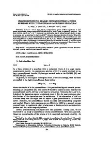
Table 3 shows the performance achieved by HOSLIM, SLIM, k-NN and HOKNN. The results show that HOSLIM produces recommendations that are better than the other methods in nearly all the datasets. We can also see that the incorporation of higher-order information improves the recommendation quality, especially in the HOSLIM framework. Moreover, we can observe that the greater the existence of higher-order relations in the dataset, the more significant the improvement in recommendation quality is. For example, the most significant improvement happens in the groceries and the synthetic datasets, in which the higher-order relations are the greatest (as seen from Table 2). On the other hand, the ctlg3 dataset does not benefit from higher-order models, since there are not enough higher-order relations. These results are to a large extent in agreement with our expectations based on the analysis presented in the previous section. The datasets for which HOSLIM achieves the highest improvement are those that contain the largest number of users and non-zeros that are covered by high-quality itemsets. Figure 1 demonstrates the performance of the methods for different values of N (i.e., 5, 10, 15 and 20). HOSLIM outperforms the other methods for all different values of N as well. We choose N to be quite small, as a user will not see an item that exists in the bottom of a top-100 or top-200 list.

k-NN HOKNN

SLIM HOSLIM

k-NN HOKNN

0.4

SLIM HOSLIM

k-NN HOKNN

1

SLIM HOSLIM

0.4

0.2

HR

HR

HR

0.8

0.2

0.6 0.4 0.2

0 5

10

15

0 20

5

10

N

15

0 20

5

N

(a) Groceries Dataset

10

15

20

N

(b) Retail Dataset

(c) Synthetic Dataset

Fig. 1: HR for different values of N.

0.35

0.32

HOSLIM SLIM

0.85

HOSLIM SLIM

HOSLIM SLIM

0.3

HR

HR

HR

0.8 0.31

0.75

0.25 10

100

1000

(a) Groceries Dataset

0.3 10

100

1000

10000

(b) Retail Dataset

0.7 10

100

(c) Synthetic Dataset

Fig. 2: Effect of the support threshold on HR.

6.3

Performance only on the users covered by “good” itemsets

In order to better understand how the existence of “good” itemsets affects the performance of HOSLIM, we computed the correlation coefficient of the percentage improvement of HOSLIM beyond SLIM (presented in Table 3) with the product of the affected users coverage and the number of non-zeros coverage (presented in Table 2). The correlation coefficient is 0.712, indicating a strong positive correlation between the coverage (in terms of users and non-zeros) of higher-order itemsets in the dataset and the performance gains achieved by HOSLIM. 6.4

Sensitivity on the support of the itemsets

As there are lots of possible choices for support threshold, we analyzed the performance of HOSLIM, with varying support threshold σ. The reason behind this is that we wanted to see the trend of the performance of HOSLIM with respect to σ. Ideally, we would like HOSLIM to perform better than SLIM, for as many values of σ, as possible; not for just a few of them. Figure 2 shows the sensitivity of HOSLIM to the support threshold σ. We can see that there is a wide range of support thresholds for which HOSLIM outperforms SLIM. Also, a low support threshold means that HOSLIM benefits more from the itemsets, leading to a better HR.

Table 4: Comparison of unconstrained HOSLIM with constrained HOSLIM and SLIM Dataset groceries synthetic delicious ml retail bms-pos bms1 ctlg3

constrained unconstrained HOSLIM HR HOSLIM HR 0.327 0.338 0.860 0.860 0.154 0.156 0.340 0.349 0.317 0.317 0.509 0.509 0.594 0.594 0.582 0.582

SLIM HR 0.259 0.733 0.148 0.338 0.310 0.502 0.588 0.581

The performance of HOSLIM under the constraint nnz(S 0 )+nnz(SHOSLIM ) ≤ 2nnz(SSLIM ) is compared to that of HOSLIM without any constraints and SLIM.

6.5

Efficient recommendation by controlling the complexity

Until this point, the model selected was the one producing the best recommendations, with no further constraints. However, in order for HOSLIM to be used in real-life scenarios, it also needs to be applied fast. In other words, the model should compute the recommendations fast and this means that it should have non-prohibitive complexity. The question that normally arises is the following: If we find a way to control the complexity, how much will the performance of HOSLIM be affected? In order to answer this question, we did the following experiment: As the cost of computing the top-N recommendation list depends on the number of non-zeros in the model, we selected from all learned models the ones that satisfied the constraint: nnz(S 0 ) + nnz(SHOSLIM ) ≤ 2nnz(SSLIM ). (9) With this constraint, we increased the complexity of HOSLIM a little beyond the original SLIM (since the original number of non-zeros is now at most doubled). Table 4 shows the HRs of SLIM and constrained and unconstrained HOSLIM. It can be observed that the HR of the constrained HOSLIM model is close to the optimal one. This shows that a simple model can incorporate the itemset information and improve the recommendation quality in an efficient way, making the approach proposed in this paper usable, in real-world scenarios.

7

Conclusion

In this paper, we revisited the research question of the existence of higher-order information in real-world datasets and whether its incorporation could help the

recommendation quality. This was done in the light of recent advances in the topN recommendation methods. By coupling the incorporation of higher-order associations (beyond pairwise) with state-of-the-art top-N recommendation methods like SLIM, the quality of the recommendations made was improved beyond the current best results.

References 1. Gediminas Adomavicius and Alexander Tuzhilin. Toward the next generation of recommender systems: A survey of the state-of-the-art and possible extensions. Knowledge and Data Engineering, IEEE Transactions on, 17(6):734–749, 2005. 2. Rakesh Agrawal, Ramakrishnan Srikant, et al. Fast algorithms for mining association rules. In Proc. 20th Int. Conf. Very Large Data Bases, VLDB, volume 1215, pages 487–499, 1994. 3. Fabio Aiolli. A preliminary study on a recommender system for the million songs dataset challenge. PREFERENCE LEARNING: PROBLEMS AND APPLICATIONS IN AI, page 1, 2012. 4. Tom Brijs, Gilbert Swinnen, Koen Vanhoof, and Geert Wets. Using association rules for product assortment decisions: A case study. In Proceedings of the fifth ACM SIGKDD international conference on Knowledge discovery and data mining, pages 254–260. ACM, 1999. 5. Paolo Cremonesi, Yehuda Koren, and Roberto Turrin. Performance of recommender algorithms on top-n recommendation tasks. In Proceedings of the fourth ACM conference on Recommender systems, pages 39–46. ACM, 2010. 6. Mukund Deshpande and George Karypis. Item-based top-n recommendation algorithms. ACM Transactions on Information Systems (TOIS), 22(1):143–177, 2004. 7. Jerome Friedman, Trevor Hastie, and Rob Tibshirani. Regularization paths for generalized linear models via coordinate descent. Journal of statistical software, 33(1):1, 2010. 8. Jonathan L Herlocker, Joseph A Konstan, Al Borchers, and John Riedl. An algorithmic framework for performing collaborative filtering. In Proceedings of the 22nd annual international ACM SIGIR conference on Research and development in information retrieval, pages 230–237. ACM, 1999. 9. Santosh Kabbur, Xia Ning, and George Karypis. Fism: Factored item similarity models for top-n recommender systems. 2013. 10. Xia Ning and George Karypis. Slim: Sparse linear methods for top-n recommender systems. In Data Mining (ICDM), 2011 IEEE 11th International Conference on, pages 497–506. IEEE, 2011. 11. Rong Pan, Yunhong Zhou, Bin Cao, Nathan Nan Liu, Rajan Lukose, Martin Scholz, and Qiang Yang. One-class collaborative filtering. In Data Mining, 2008. ICDM’08. Eighth IEEE International Conference on, pages 502–511. IEEE, 2008. 12. Francesco Ricci and Bracha Shapira. Recommender systems handbook. Springer, 2011. 13. Robert Tibshirani. Regression shrinkage and selection via the lasso. Journal of the Royal Statistical Society. Series B (Methodological), pages 267–288, 1996. 14. Zijian Zheng, Ron Kohavi, and Llew Mason. Real world performance of association rule algorithms. In Proceedings of the seventh ACM SIGKDD international conference on Knowledge discovery and data mining, pages 401–406. ACM, 2001.