International Joint Conference on Autonomous Agents and Multiagent Systems (AAMAS), Hakodate, Japan, 2006: 646-653
How Autonomy Oriented Computing (AOC) Tackles a Computationally Hard Optimization Problem Xiao-Feng Xie
Jiming Liu
Department of Computer Science Hong Kong Baptist University Kowloon Tong, Hong Kong
Department of Computer Science Hong Kong Baptist University Kowloon Tong, Hong Kong
[email protected]
[email protected]
ABSTRACT The hard computational problems, such as the traveling salesman problem (TSP), are relevant to many tasks of practical interest, which normally can be well formalized but are difficult to solve. This paper presents an extended multiagent optimization system, called MAOSE, for supporting cooperative problem solving on a virtual landscape and achieving high-quality solution(s) by the self-organization of autonomous entities. The realization of an optimization algorithm then can be described in three parts: a) encode the representation of the problem, which provides the virtual landscape and possible auxiliary knowledge; b) construct the memory elements at the initialization stage; and c) design the generate-and-test behavior guided by the law of socially-biased individual learning, through tailoring to the domain structure. The implementation is demonstrated on the TSP in details. The extensive experimental results on real-world instances in TSPLIB show its efficiency as comparing to other algorithms.
Categories and Subject Descriptors I.2.8 [Problem Solving, Control Methods, and Search]: heuristic methods; I.2.11 [Distributed Artificial Intelligence]: multiagent systems
General Terms Algorithms, Experimentation, Theory
Keywords Multiagent system, Autonomy Oriented Computing (AOC), Traveling Salesman Problem (TSP), global optimization, search, cooperative problem solving, emergent and collective behavior.
1. INTRODUCTION The hard computational problems are ubiquitous in scientific and engineering fields [26], which often are conceptually simple and can be cast as a search through a space of alternatives [24][37].
Permission to make digital or hard copies of all or part of this work for personal or classroom use is granted without fee provided that copies are not made or distributed for profit or commercial advantage and that copies bear this notice and the full citation on the first page. To copy otherwise, or republish, to post on servers or to redistribute to lists, requires prior specific permission and/or a fee. AAMAS’06, May 8–12, 2006, Hakodate, Hokkaido, Japan. Copyright 2006 ACM 1-59593-303-4/06/0005...$5.00.
The landscape paradigm originated in theoretical biology is used for search in general [25]. Suppose the representation space (SR) G contains all the potential solutions, where each is called a state s , and the solution space (SO) is a set of states with reasonable quality. Normally, the SO/SR is quite small since that the size of SR expands exponentially with the size of problems [24]. For the G optimization task to find s ∈ SO with high probability, typical challenges include: a) little a priori knowledge is available; and b) total computational resource and time are bounded. The traveling salesman problem (TSP) [40] is a classic NP-hard problem. Although the TSP is easily formulated, it exhibits various aspects of hard computational problems and has often served as a touchstone for new problem solving methods [29][54]. The researches [10][17][53] have indicated the phase transitions under certain order parameter(s), however, it seems most realworld instances are still located at the hard computational region. Autonomy oriented computing (AOC)[31] addresses the modeling of autonomy in the entities of a complex system and the selforganization of them in achieving a specific goal. The complex behaviors can emerge from the interactions of autonomous entities following simple rules. Recently, the AOC based methods have been applied to solve various problems [30][47][51]. In this paper, the compact multiagent optimization system (MAOSC) [51], which is originally proposed for handling with the numerical optimization problem (NOP) only, is extended for supporting the cooperative search on a virtual landscape by a society of compact agents with limited memory capacity and simple behavioral rules under ecological rationality [18]. Each agent only has moderate problem solving capability by comparing with two extremes: a) the reflex agent, such as ant [12], which has no declarative memory and can only produce reflex behaviors in the environment; b) the cognitive architecture, such as ACT-R [1], which is rather sophisticated under unbounded rationality. Besides, the cooperation [13] is necessary because no single agent has sufficient knowledge on the virtual landscape. Here the agents collaborate with the others by indirect interactions, which are implemented through the communication medium role of the environment [31], instead of by sophisticated negotiation [27]. The paper is organized as follows. In Section 2, the extended multiagent optimization system (MAOSE) in two levels is introduced in details. In Section 3, the implementation is demonstrated on the TSP, which addresses exploiting the problem features in search. In Section 4, the extensive experimental results by MAOSE, using real-world instances from the TSPLIB, are
compared with those of some existing algorithms [45][54]. In the last section, this paper is concluded.
2. THE MULTIAGENT SYSTEM The extended multiagent optimization system is built in two levels: a) the symbolic level for supporting basic problem solving; and b) the multiagent framework for specifying the organization structure and operation mechanism based on the symbolic level.
2.1 The symbolic level The general problem solving capability arises from the consequence of the interaction of declarative and procedural knowledge [1]. As in the information process system [37], the declarative knowledge is represented in symbol structures, called T_INFO elements, and the procedural knowledge is represented in elementary information processes, called behavioral rules. Each T_INFO element is described by a tuple , where I_RC is the retrieve cue, I_TYPE indicates a certain search space, and I_CON is its state. The memory [19][37] is used for storing T_INFO elements. Each element can be retrieved from a memory according to its I_RC. The memory must be updated if it is to be useful [19]. But updating is not encoding a new T_INFO element. Instead, only the I_CON is subjected to change. Then a T_INFO element can be referred as a trajectory that comprise of many instances. For (t ) specified time t, a T_INFO instance is expressed as I_TYPE I_RC .
Each behavioral rule is described by a tuple , where I_KEY indicates a virtual interface for handling specific T_INFO elements, and I_NAME indicates the real operations, which can be controlled by specifying setting parameters within a I_NAME
rule-parameter space. A behavioral rule is expressed as RI_KEY
.
2.2 The multiagent framework As an AOC-based model [31], the framework consists of a society of N agents where they cooperate in a sharing environment (E) to realize a common intention of finding high-quality solution for an optimization task. Since the optimization task can be well-defined, the sophisticated negotiation [27] among agents is not necessarily. Instead, an agent is communicated with the others by indirect interactions, which are implicit implemented through the communication medium role of the environment (E). Agent
Central Executive
MA
(private)
RCO
Generate-and-test behavior
(socially biased individual learning)
MS
(social sharing)
FR
Environment (E)
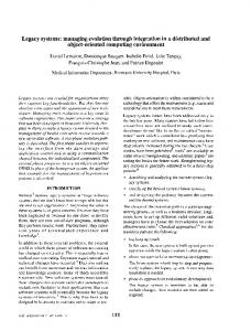
Figure 1. An agent and the environment (E) it roams
Without loss of generality, the agents are homogenous in the sense that they have the same organized structure. Figure 1 shows one of the agents and the environment it roams. All other agents are interacted with the environment in same way.
2.2.1 Environment The environment serves as the domain in which agents roam [31]. Firstly, it contains an internal representation (FR) [36][41] of the optimization task, which encapsulates accessible rudimental knowledge, includes a virtual landscape [25] and some auxiliary information associated with problem structure. For the landscape, a quality evaluation rule (RM) is used for measuring which one has better quality between any two states G ( s ) in the representation space (SR). The quality evaluation implies the intention to attain the state that is better than another. G For normal problems, there is a cost function f( s ) for each state G G G s ∈ SR. Then the evaluation is realized by a RMO ( sa , sb ) rule: G G G G G for ∀ sa , sb ∈ SR, if f( sa ) ≤ f( sb ), then the sa is better than the G sb , and RMO returns TRUE, else it returns FLASE. Secondly, the environment holds a socially-shared memory (MS), called collective memory [38], which serves as the blackboard for all agents by creating a shared past. The information flow from the agents to the MS is supported by the coordinating behavior (RCO) as in Fig. 1. In this sense, the environment also serves as an accumulation pool for the emergent collective behavior instead of a pure information provider as in cognitive architectures [1]. Thirdly, the environment keeps a central clock that helps synchronizing the behaviors of the total system, if necessary [31]. In fact, the environment can be seen as a pseudo autonomous entity for supporting the indirect cooperation of agents.
2.2.2 Agent Each agent is a socially situated autonomous entity. Autonomy [31] is an attribute of a self-governed, self-directed entity with respect to its own status, free from the explicit control of another entity. The essence is that each entity is able to make decisions for itself, subject to the limitations of the available information. The central executive (CE), the most important component of working memory model [3][43] in term of its general impact on cognition, is responsible for manipulating the local behavior and behavioral rules of an agent, which govern how it should act or react to the available information on the representation of problem while determine the next status to which the entity will transit. The agent has two belief sources. Firstly, it possesses a private memory, called MA, which has limited capacity and can only be modified by agent itself. The MA is a fundamental mental component for supporting individual learning. Secondly, it can access to the MS, which is socially available from the environment. The law of behavior is socially biased individual learning (SBIL) as adopted by many species in real world [16], which is a mix of reinforced practice of own experience and socially available information. The SBIL is suggested to be a heuristic in ecological rationality [8][18], which a) gains most of the advantages of both individual and social learning; and b) facilitates the emergent and
collective properties by allowing learned knowledge to be accumulated from one generation to the next.
TSP landscape and a candidate set for accelerating the local search (LS), the basis of many good heuristic methods.
Due to lack of enough knowledge on the landscape to be searched, the essential behavioral rule is generate-and-test rule (RGT). The essential components of an RGT rule include a generating part (RG), a solution-extracting part (RS) and a testing part (RT) [51]. The RS part has no influence on the problem-solving process. It just exports potential solution(s) during a run. Without loss of generality, it can be supposed that only the RG part can create new information that contains new potential solution(s), and the RT part only produces simple reflex behavior, which may determine nontrivial properties for some T_INFO elements in memory.
3.1.1 The TSP landscape
2.2.3 Working process The framework runs in two phases. The first phase is memory initialization phase, which initializes the T_INFO elements in MS and in the MA of all agents according to the FR. The second phase is generate-and-test phase. For a run, the number of cycles is T. The behavior of system in the tth ( t ∈ [1, T ]] ) cycle only relies on the status of system in the (t-1)th cycle. By running as a Markov chain process, the system can be analyzed in each cycle. Each cycle contains two clock steps: the C_PRE and the C_RUN. At the C_PRE step, the coordinating behavior (RCO) at the environmental level, which summarize the information submitted by all the agents into the MS, is executed, i.e. {M A((t i))
| i ∈ [1, N ]] },
M S(t )
→ M S(t +1) RCO
(1)
For simplicity, here only the observational information is taken into account, i.e. the T_INFO elements in all agents with same I_RC are collected into a T_INFO element in MS. It is significant since observational learning [5] can lead to cumulative evolution of knowledge that no single agent could invent on its own. At the C_RUN step, if an agent is activated, where its generateand-test rule is executed for generating new information by estimating the distribution of promising space according to available information in MA and MS and updating its MA, i.e., G (2) {s (t ) } RGT → M A(t ) , M S(t ) (t +1) M A Naturally, there are two run modes: a) full-run mode, where all agents are activated; b) partial-run mode, where only NACT agents (NACT ∈ [1, N ]] ), which are selected at random, are activated. Under same agent activated times, the system in partial-run mode often converges fast since it allows fast information diffusion.
3. IMPLEMENTATION FOR THE TSP For solving the TSP, the implementation is realized in three steps: a) define the representation of the TSP (FR); b) initialize the memory; and c) design suitable generate-and-test behavior. According to no free lunch theorem [50], the domain knowledge of the problem must be embedded at the implementation stage.
3.1 Representation of the TSP (FR)
The representation (FR) provides a basic interface for accessing the essential domain information of the TSP, which includes a
The TSP landscape is quite straightforward. It is a weighted complete graph with V nodes (or called cities) and a cost matrix D=(dij), where dij represents the length of an edge that connects between cities i an j (i, j ∈ [1, V] ] ). Here we only concern with the symmetric TSP, which have dij = dji for every pair of nodes. The TSP then is to find a minimal-cost Hamiltonian tour that G passes through each node once. Each state s is a complete tour, which can be represented as a permutation (i1, i2, …, iV) of the integer values from 1 through V, where the cost function is G f ( s ) = d i1 i2 + d i2 i3 + ... + d iV i1
(3)
The distance of two states is defined as the number of edges in which they differ [15][29][34]. In this paper, the original TSP landscape is used in order to allow a fair evaluation of the performance of algorithms. However, it should be mentioned that the transformation of the cost matrix always be an approach for improving the solving performance. One kind of methods does not change the relative order of the states. As in Lagrangean relaxation [23][40], the length of every tour is increased by 2 ⋅ ∑ π i as we associate with each node i a penalty value π i and use the transformed cost matrix D’=( d ij' ), where d ij' = dij+ π i + π j . Of course, the order for the same segments of a tour may be changed under different cost matrix. The other kind of methods indeed changes the global landscape. As in search space smoothing [21], the original landscape is transformed into a series of gradually smoother landscapes, which the smoothest one is solved at first and the solutions are used for guiding the following landscapes until the original one.
3.1.2 Candidate set (EC) for local search
Local search (LS), also known as neighborhood search, has been shown very effective for hard computational problems, including the TSP. A basic LS algorithm, under a predefined candidate set of neighborhood description, starts from an arbitrary complete tour and repeatedly improves the current tour till it is trapped into a local minimum. 2-Opt, 3-Opt and Lin-Kernighan (LK) algorithm [29] are representative LS methods. The complete graph for a symmetric TSP has (V2-V)/2 edges. However, it is intuitively that most of the possible edges will not occur in good tours because they are simply too long [40]. It is therefore reasonable to restrict major attention to promising edges, or called the candidate set, for accelerating local search (LS) methods. The examples of candidate sets include the k (k≥1) nearest neighbor subgraph, and the Delaunay graph, etc [40]. Of course, it is often expected the candidate set to be smaller so as not to result in a substantial increase in running time. Helsgaun [23] estimates the chances of a given edge being a member of a good tour by using minimum 1-trees [40]. A 1-tree is a spanning tree with an additional edge combined two nodes with degree 1. The minimum 1-tree is often used for estimating the lower bound on the optimum since it is a relaxation of the TSP. The estimation, or called Held-Karp bound [22], can be improved
substantially on the 1-tree with Lagrangean relaxation [40] by applying subgradient optimization [22] for determining a certain transformation of the cost matrix with the suitable set of penalties, which each π i is associated with each node i. In α-nearness measure [23], each edge has a corresponding αvalue, which is the minimum length when a 1-tree is required to contain the specified edge based on a transformed cost matrix. Intuitively, the more accurately Held-Karp bound achieved by the transformed cost matrix, the better estimation of α-values for the edges. Then the candidate edges of each node are sorted in ascending order of their α-values. Usually the minimum 1-tree shares many edges with an optimal tour. It is intuitive that the smaller α is for an edge, the more promising is this edge.
3.1.3 The features of the TSP landscape The landscape is often studied in various ways. The first way is to understand the landscape in terms of simple parameters [44], in particular, to depict the phase transitions according to certain order parameters [10][17][24][53]. For the TSP, most researches are focused on the matrix D. Chessman et al. [10] investigated the standard deviation of the D as an order parameter by using a backtrack algorithm. Zhang [53] went deep into the precision of the elements in the D by using a branch-and-bound algorithm. The phase transitions in many hard computational problems have revealed interesting regularities across different problems and algorithms [24]. However, most real-world TSP instances are still classified as hard at the existing phase diagrams. The second way is to understand the landscape based on the hints accumulated from the solving experience of existing algorithms. Most modern LS variants [2][23][32][45] are essentially under the umbrella of iterated LS (ILS) [32], or called chained LS (CLS) [2], where the basic idea is to modify the current tour by applying a kick-move on a previous found tour instead of independently generated one. The intuition behind using chained starting tours is that the strong positive correlation between solution cost and the distance from the closest optimal tour, i.e., better local minima tend to have smaller distance to the closest global optimum by sharing many common partial structures [7][32][54]. The observations have led to the “big valley” hypothesis [7], which argues that the high-quality tours tend to concentrate on a very small subspace around the optimal tour(s) [46]. Moreover, the inherent features of a set of high-quality tours have been exploited in several ways. The first is reduction [29], which locks the edges in the intersection of the edge sets (EI) of the tours for speeding up the subsequent search. However, this method is brittle [54], especially as a locked edge is not part of good tour. The second is tour merging [11], which is to look for a highquality tour in a restrict graph (GR) consisting of the union of the edge sets (EU) of the tours through a “branch-width” algorithm. In fact, the number of edges in a GR can be quite few due to the large number of shared edges among high-quality solutions. However, optimizing over a GR can be hard as the original TSP instance. Besides, although a GR may contain most of edges of an optimal tour, it may not ensure containing at least one optimal tour, then the tour merging may be failed to achieve optimum. The third is backbone guided search [54], which makes using of global information embedded in the pseudo-backbone frequencies for changing the landscape. However, the local search may be trapped into a local minimum unaffected by the changed landscape.
In this paper, the TSP landscape is exploited in the following ways: a) the LS method is applied at the initialization (or early) stage in order to reach the “big valley” as soon as possible [7]; b) The new tour(s) are generated based on the kick-move on a previous found tour as in the iterative LS [32]; c) an edge set (EU), which is represented in a set of high-quality tours, are used as the guiding information for the kick-move. The basic idea is that, for the edges to be introduced, most of them come from the EU and a few of promising edges are safely introduced by greedy search. Moreover, to use a EU with repeated edges instead of a restrict graph may utilize the pseudo-backbone frequencies implicitly; and d) the diversity among tours is maintained carefully: firstly, each starting tour is conserved in the private memory of each agent; secondly, the partial instead of the full information in EU, normally be a single tour, are used for guiding the kick-moves; and thirdly, the diffusion distance for each starting tour is restricted by an additional testing criterion on multiple trails.
3.2 Memory initialization For simplicity, We use one T_INFO element in MA, i.e. a tour G (t ) G G called sP(t ) . Hence the element in MS is $sP( t ) ={ sP (i ) | i ∈ [1, N] ] }. Following a random initialization, each tour is improved by a LS method, indicated as LSMI. The default choice for LSMI is a 3-Opt with kNNI=20 neighborhood nodes in the candidate set.
3.3 The generate-and-test behavior For solving the TSP, the generate-and-test behavior can be seen as G a kick-move on sa , the starting tour to be improved, as in ILS [32]. To improve the chances for escaping from the local optimal tours, the double-bridge (DB) [29][32], a non-sequential kick-move, is normally used [2]. Helsgaun [23] has extended it into a 2-stage kick-move, i.e., any infeasible 2- or 3-Opt move (producing an intermediate solution consisting sub-tours) followed by any 2- or 3-Opt move, which produces a valid tour (by merging the subtours). The infeasible intermediate solution is significant so as to alter the global shape of a tour [2]. However, the blind mutation should be avoided since it may be ineffective and inefficient. The kick-move guided by a high-quality edge set (EU) has been exploited extensively. Many of them [15][28][34][42] can be classified as the tour-guided 2-stage kick-move (TG2KM): guided G G by a tour sb in EU, the tour sa is first modified into an infeasible intermediate solution, normally consist disjoint segments or subtours, which are then repaired by ingenious greedy mechanisms while considering available information, such as the EC. Many edge-based recombination operators, such as Voronoi Quantized Crossover (VQX) [42], Natural Crossover (NX) [28], Distance Preserving Crossover (DPX) [15], Edge Assembly Crossover (EAX) [34][35], etc., can be taken as the examples. Guiding by a tour instead of mutating blindly brings an implicit G G advantage by utilizing the distance between sa and sb . Normally, G the larger distance, the large perturbation on sa is then allowed. It brings an adaptive control of the balance between exploration and exploitation along with the execution cycles. Using a single tour instead of the whole information available is simply because the former has inherent mechanism for preventing premature convergence by locally diffusion of information in a
self-organized agent network while the latter needs sophisticated mechanism although it provides more complete information. Normally, new promising edges can only be safely introduced when repairing the intermediate solution in greedy way. Hence the unexpected edges that are introduced into the intermediate G solution, which are not existed in the sb and the set EC, should be as less as possible. The following RGT rule, called RGTEA , is extended from the EAX [34], because it meets the requirement.
3.3.1 The generating behavior The generating part (RG) is applied for generating new tour(s). The preliminary operation is to build the mappings between the G external and internal information sources, i.e., from the sP(t ) and G G the $sP( t ) to the starting tour sa and the guiding edge set EU. Here G (t ) G sa = sP so as to preserve information naturally by using the
G
private memory; and EU= $sP( t ) so as to make use of the cumulative G G pool. Moreover, the sb is a tour selected from the $sP( t ) at random so as to utilize the pseudo-backbone frequencies implicitly. G G By defining the GAB as a graph constructed by merging sa and sb , the edges on GAB are then divided into AB-Cycles [35], where an AB-cycle is defined as an even-length sub-cycle on GAB generated G G by tracing different edges of sa and sb alternately. As an ABCycle is identified, then the edges making up the AB-Cycle are removed from GAB and the AB-Cycle is stored into the AB-Lib if G G it contains not only common edges of sa and sb . The procedure is repeated till no AB-Cycle could be extracted. Each AB-cycle in AB-Lib can be used as the guiding information G for applying a kick-move on sa in two steps [35][49]. The first step is to generate an intermediate solution, i.e., by G G removing edges of sa in the AB-cycle from sa and adding edges G G of sb in the AB-cycle to sa . The result is a set of disjoint subG tours. It is obviously that all the changed edges of sa are selected G G from sb . Besides, the edges in sa will be unchanged in the G intermediate solution if the edges that connected to a node in sb G belong to the edges that connected to the same node in sa . The second step is to modify the intermediate solution into a valid tour by merging its sub-tours. Of course, it is a choice to apply the 2-Opt for merging sub-tours [9]. For reducing the computational cost, a LS version, which can be seen as the first round of 2-Opt, is used [34]: two sub-tours are greedy merged, by deleting one edge from each sub-tour and adding two edges, where one of them is a node selected at random in the candidate set EC, to connect the nodes in both sub-tours with degree 1. Of course, to find a good tour by simple one trail is not always easy. Fortunately, there already are many AB-cycles in the ABLib, which allows us to perform a multi-trail mechanism (MTM), or called iterative child generation (ICG) [35][49], i.e. to generate NMTM candidate tours, where each is based on an AB-Cycle selected in AB-Lib at random. The idea was also exploited by the Fitness-Distance-Based Diversification (FDD) [45] and the brood selection mechanism [48]. The default value for NMTM is set as 30.
3.3.2 The testing behavior The testing part (RT) is used for maintaining the MA, which is similar as updating the starting solution in iterated LS, based on the competition among the generated candidate tours. The smaller difference between two information sources for the RG part, the higher probability for falling into one of the local minima associated with the guiding information [7][15]. Hence, it is critically to maintain the diversity of information intentionally since the high-quality solutions are already rather close. For the competition of generated tours, it may easily get trapped in specific regions of the TSP landscape if we only consider the essential high-quality criterion [49]. The FDD mechanism [45] hence utilizes an additional criterion, i.e., high quality as well as rather distant from the starting tour. G G If sa is located at a local valley, then a tour better than sa is located at another valley of the TSP landscape. Here if only such tours are allowing for competition, then it is no long necessarily to keep large distance from the current solution intentionally. It is expected that the private information in MA has strong influence on the generated states, so as to keep a local diffusion effect. Hence large adjustments are possible, but are much less G probable than small adjustments [4]. For a generated tour sc with
G
better quality than sa , the cost function is transformed as follows:
G G G G G f '( sc) = ( f ( sc ) − f ( s a )) /( DIS ( s a , s c )) C D
(4)
G G
where DIS ( sa , sc ) is a function to reflect the increasing of
G
G
distance between sa and sc , and CD is called diffusion coefficient. G G As in [34], the DIS ( sa , sc ) function is defined as half of the number of edges in the corresponding AB-cycle to reduce computational cost for calculating the exact distance.
G
If CD=0, f '( sc) represents the high-quality criterion, as in EAX1AB [34][35] or in brood selection mechanism [48]. If CD=1, G f '( sc) represents the criterion as in EAX-Dis [35]. If CD is very
G
large, the sc will be selected from the tours with smallest DIS value. In fact, the CD determines the diffusion velocity of information. The default setting is CD=1.5. G G The selected sc is then used for replacing the sP(t ) in MA. Hence
G xP is a steady-state solution satisfying the above testing criterion.
4. EXPERIMENTAL RESULTS The experiments are carried out on a set of real-world instances with 1000≤V