PHYSICAL REVIEW E 76, 031919 共2007兲
How disease models in static networks can fail to approximate disease in dynamic networks N. H. Fefferman1,2 and K. L. Ng3,2,*
1
InForMID, Tufts University School of Medicine, 136 Harrison Avenue, Boston, Massachusetts 02111, USA 2 DIMACS, Rutgers University, 96 Frelinghuysen Road, Piscataway, New Jersey 08854, USA 3 Department of Mathematics, 2 Science Drive 2, National University of Singapore, Singapore, 117543 共Received 19 February 2007; revised manuscript received 22 July 2007; published 19 September 2007兲
In the modeling of infectious disease spread within explicit social contact networks, previous studies have predominantly assumed that the effects of shifting social associations within groups are small. These models have utilized static approximations of contact networks. We examine this assumption by modeling disease spread within dynamic networks where associations shift according to individual preference based on three different measures of network centrality. The results of our investigations clearly show that this assumption may not hold in many cases. We demonstrate that these differences in association dynamics do yield significantly different disease outcomes both from each other and also from models using graph-theoretically accurate static network approximations. Further work is therefore needed to explore under which circumstances static models accurately reflect constantly shifting natural populations. DOI: 10.1103/PhysRevE.76.031919
PACS number共s兲: 87.23.⫺n, 89.75.Fb, 87.10.⫹e, 89.75.Hc
I. INTRODUCTION
Traditional compartmental susceptible-infected-recovered 共SIR兲 models of disease spread assumed homogeneous mixing rates within an infected population 关1–3兴. However, more recently, models have been developed to examine the effects of heterogeneities in the mixing rates among individuals on patterns in the spread of infectious diseases 关3,4兴. Among the techniques employed, network models are the most explicit in their incorporation of social contacts, defining each interaction between pairs of individuals 共or groups of individuals兲 and considering these as potential routes of pathogen transmission 关3,5–14兴 共see Ref. 关14兴 for a review of network epidemiology and a list of references therein兲. The results of these studies have shown that the network structure of the population can greatly affect the duration and overall severity of an outbreak 关3,6,8,10,11,13兴. However, the underlying assumption for most of these works is that the network is essentially static: once an association is formed between two individuals this association will remain unaltered. Unfortunately, associations between individuals in a social network usually change with new relations being formed and old ones removed continuously 关15,16兴. A few studies have examined the resulting spread of disease in networks with shifting contacts 关14,17–19兴. Further, there have been several studies on the spread of disease on scale free 关13,20,21兴, small world 关22,23兴, and random 关24兴 networks. Some investigations have examined patterns of disease spread on growing networks, determining how the formation of new contacts can affect the transmission of infectious diseases 关17兴. These studies have all assumed generalized dynamic processes to determine the changes over time, maintaining the global properties of the network 共e.g., small world properties, average degree, etc.兲. However, by focusing on a local level, rather than considering the global properties of the network in its entirety, dy-
*
[email protected] 1539-3755/2007/76共3兲/031919共11兲
namic networks can be used to examine the role of individual behaviors. Nonrandom individual behavior 共in which individuals within the graph make preferential association choices based on some network structure measure; one wellknown example of such association behavior is called “preferential attachment” 关25兴兲, has already been shown to greatly affect the global structure of a network, with different association preferences potentially yielding very different emergent network structures 关26兴. These kinds of shifting networks 共i.e., those that change with time based on individual action兲 have been the focus of various studies in social network theory 关27,28兴. In particular, social network models where individuals modify their associations based on optimizing some utility function determined by the cost and benefits involved in maintaining an association were studied in Refs. 关27–29兴. However, to the best of our knowledge, no studies to date have examined the impact such individually driven network dynamics can have on the structures of networks 共regardless of whether a converging structure emerges兲, and the associated susceptibility of the population to disease threats. In order to investigate the potential role of individually driven network dynamics in infectious disease epidemiology, we adopt three simplified measures of network “centrality” 关30兴: “degree,” “betweenness,” and “closeness.” The degree centrality of an individual v is defined to be the proportion of individuals in the network to which v is affiliated. The betweenness centrality describes v’s belonging to the shortest contact paths between pairs of other individuals in the network, while the closeness centrality of v is a quantification of how many contacts away v is from all other individuals in the network. 共Details of the use of these measures in the modeling of network dynamics, in addition to the use of associated metrics for describing the centrality of the network as a whole, are discussed in Appendixes A and B, but also see Ref. 关26兴.兲 Incorporating the use of centrality measures in the study of network disease epidemiology is not novel, as observed in Refs. 关31–33兴. However, we do not here propose to characterize the explicit nature of disease spread by the use of these measures, instead we use central-
031919-1
©2007 The American Physical Society
PHYSICAL REVIEW E 76, 031919 共2007兲
N. H. FEFFERMAN AND K. L. NG
ity only as a proxy system for network dynamics based on individual preference. There are examples of populations in the natural world in which individuals are seen to form associations based on characteristics consistent with both the degree and the closeness measures of centrality 共see Ref. 关26兴, and references therein兲. Of course, these measures most certainly do not capture the full complexity of social systems and are only three of the many centrality measures employed by social network theorists. These measures are used here only as a reasonably diverse set of measures, yielding substantially different outcomes for the same individuals within the same network. They are merely employed because, together, they represent a sufficient diversity in the complexity of individual evaluative capability so as to provide an initial point of investigation into how constantly shifting dynamics could have an effect on the resulting network structure which could then, consequently, affect disease dynamics on the network. Additionally, in traditional and static network models, higher probabilities of transmission of infection from an infected to a susceptible individual have been shown to increase the severity of an outbreak up until a saturation threshold past which the disease reach density dependent feedback based on the remaining number of susceptible individuals 关3,13兴. In a dynamically shifting network, however, the possibility arises that the relative rates of shifting social contacts and transmission of infection could together produce different patterns of disease spread, causing disease load 共the cumulative number of secondary infections occurring in a population over a period of time兲 to no longer vary directly in proportion to the probability of transmission. This could then lead to different relative susceptibilities of different dynamic populations under different probabilities of transmission. The existence of such relative differences would reveal yet another important effect of dynamic social contact networks. Although it may prove to be impossible to characterize social networks and their dynamics in human populations, how such dynamics can affect the accuracy of disease models employing static approximations would provide crucial insight into any true understanding of the behavior of infectious disease. Any increase in understanding how the continual shifting of contact patterns within populations can affect network structures may lead to a greater understanding of how these structures affect disease incidence and may ultimately improve potential intervention strategies. If dynamic networks do not uniformly converge to structures 共e.g., exhibiting scale free properties, having power law degree distributions兲, then any difference in disease incidence between dynamic and static models would suggest that network dynamics can have a profound effect. Additionally, many of the diseases of modern concern emerge from wildlife populations in which population size is relatively small and social behavior is well studied 共and, for some species, even well represented by these sorts of simple centrality measures; e.g., degree centrality as in Ref. 关34兴; cf. Ref. 关26兴兲 and could easily be characterized for purposes of modeling. In using mathematical models to understand the complicated processes of disease in wildlife and human populations no one facet is likely to be solely responsible for
driving the dynamics but social dynamics may prove to play a significant and substantial role. As with our choice of centrality measures, the characteristics we have chosen to ascribe to our social networks are not meant to accurately represent specific characteristics of any particular real-world networks. We have examined relatively small networks, using individual social preferences based on local information 共centrality of neighbors兲 derived from global standing within a closed community to investigate whether or not a set of dynamic behaviors exist which cause disease spread to behave in ways unpredicted by studies on static networks. Here we provide an investigation into the spread of disease in these individually driven dynamic social networks. II. METHODS
To model an association network of N individuals 共see Table I for a summary of parameters and variables used in this study兲, we use a directed graph 共or digraph; a graph in which the direction of edges, then called “arcs,” from one individual to another is specified兲 in which each individual was assigned five out neighbors 共arcs originating from the individual兲 as described in the methods of Ref. 关26兴, details of which are provided in Appendix A. A digraph was utilized to reflect the fact that not all social relationships are reciprocal 共e.g., hierarchical grooming, see Refs. 关12,36兴兲. The association preference 共betweenness, closeness, or degree; see Refs. 关26,30兴兲 for all individuals within a population was defined prior to the beginning of the computation. The network then shifted as each individual kept three and discarded two of its out-neighbors according to their relative rank under the appropriate measure in each computational time step before replacing the two discarded neighbors with two others in the network chosen at random. Thus the number of arcs in each network is kept constant during each time step 共again see Appendix A兲. 共Note: in order to agree with the notation of social network theory, the measure of “popularity” from Ref. 关26兴 will here be referred to as “degree.”兲 We refer to a population where all the individuals having betweenness 共closeness and degree兲 as an association preference, as a B population 共C and D populations兲. In order to compare the stochastic process of disease spread consistently over these divergently shifting networks it is necessary to ensure that contact 共an arc兲 between a specific susceptible and infected pair of individuals, resulting in the successful transmission of disease in one network, will also result in transmission in any other network in which the disease status and contact within the pair is identical within the same computational time step. To accomplish this, we define G to be the complete digraph 共containing all possible arcs兲 with N individuals. In each time step, our networks can thus be considered to be separate subdigraphs of G 共Gt,B, Gt,C, and Gt,D for the B, C, and D populations at time t, respectively兲 where all individuals in G exist in each of the three subdigraphs even though many of the arcs do not. To ensure that only the association preferences affected the network structures over time, a single subdigraph was generated at random and all three networks were initially defined to be equal to that single subdigraph. Therefore G0,B = G0,C
031919-2
PHYSICAL REVIEW E 76, 031919 共2007兲
HOW DISEASE MODELS IN STATIC NETWORKS CAN…
TABLE I. A summary of parameters and variables used in this study. Variable/parameter
Description
Value共s兲 taken
N t
Number of vertices in network Discrete time step
t*
Time step when primary source of infection is introduced into model
Inf.-dur.
Number of time steps a vertex in state I stays infectious before returning to state S Additive factor if reciprocal arc exists between a vertex in state I and another in state S Probability of successful transmission of infection from vertex in state I to a neighboring vertex in state S
50a 0 , 1 , . . . , 200 共for dynamic model兲 0 , 1 , . . . , 250 共for static model兲 50 共for dynamic model兲 100 共for static model兲a 2
Add.-fact. Ptrans
0.2 0.05, 0.1, 0.15, 0.2a
a
Indicates that these values were altered to examine the effects of different network sizes on the results; scaled outcomes are reviewed briefly in Appendix D.
= G0,D 債 G, although subsequent shifting within each of the networks would result in divergent network structures among the three populations already after the first computational time step. In order to model the spread of infectious disease in each of these three dynamic networks, we classify each individual as either susceptible 共S兲, exposed 共E兲, or infected 共I兲. 共Our models can thus be considered a network-based representation of the standard SEIS model; see Ref. 关35兴.兲 All individuals are initially susceptible. A single individual vk 苸 G was chosen at random at t = t* through which infection was introduced into each of the three networks G50,B, G50,C, and G50,D, even though by then these three networks would have very different network structures 关26兴. This single point source was the only instance of primary disease introduction into the population. All subsequent infections were the result of secondary transmission, described as follows. In each t ⱖ t*, we generated a single N ⫻ N matrix M t 关with the 共i , j兲 entry of M t denoted by M ti,j and taking values between 0 and 1 chosen from a uniform distribution兴. For ease of notation, within each network type X, we define at,X共i , j兲 to be equal to 1 if vi is adjacent to v j in Gt,X and zero otherwise. At each t, if an individual vi is in state I, another individual v j is in state S, then transmission of infection occurs if either 共a兲 at,X共i, j兲 = 1,
at,X共j,i兲 = 0,
M ti,j ⱕ Ptrans
or
共b兲 at,X共i, j兲 = 0,
at,X共j,i兲 = 1,
M tj,i ⱕ Ptrans
or
共c兲 at,X共i, j兲 = 1, at,X共j,i兲 = 1, M ti,j + 共Add.-fact.兲M tj,i ⱕ Ptrans , where Ptrans is the constant probability of transmission given contact between a susceptible and an infected individual. This successful transmission of disease caused the susceptible individual to be considered exposed for one time step and subsequently to become infectious at the beginning of
the next time step 共this was done for ease of implementation and not due to any disease specific properties of investigation兲. The individual then remained infected for Inf.-dur. time steps and then returned to being susceptible. Note. For the purpose of disease transmission, there was no difference between an arc from vi to v j and one from v j to vi. If either one of the two arcs 共but not both兲 existed between vi 共in state I兲 and v j 共in state S兲, then it was equally likely for vi to infect v j regardless of the direction of the arc. However, if both arcs existed, the probability of a successful disease transmission was adjusted by a factor of Add.-fact. as described above. Thus while individual associations were altered based on a digraph structure, the processes of disease spread occurred on an undirected network. As a result, the disease propagation model employed allowed for transmission in either directions of the association between two individuals so long as any association between them exists. While the social association network structure was a digraph, the disease propagation network structure was an undirected graph. We believe that this allows us to reasonably approximate both the asymmetric social and bidirectional disease dynamics. Defined as above, M ti,j can be thought of as representing an independently generated random value governing whether or not disease would be transmitted from vi to v j in the complete digraph G. Therefore, though each arc in G may not exist within all of the three subdigraphs at a given t, if an arc existed between two individuals vi and v j in more than one of the subdigraphs during the same computational time step, it carried the same associated M ti,j. As a result, the transmission of infection between two individuals at any particular computational time step was consistent across all three dynamic networks so long as the arc between the pair existed in the corresponding subdigraphs. In this way, we controlled for the stochastic effects of the disease propagation model, allowing us to compare disease spread among the divergent network structures over time 共see Fig. 1兲.
031919-3
PHYSICAL REVIEW E 76, 031919 共2007兲
N. H. FEFFERMAN AND K. L. NG
The complete digraph with all possible arcs G ⊇ {G0, B = G0,C = G0, D } The sub-digraphs with only the arcs among individuals among all 50 individuals dictated by their specific affiliation dynamic Affiliations shift depending on individual preference
(A)
G ⊇ {G49, B
≠
G49,C
≠
G49, D }
G ⊇ {G50, B
≠
G50,C
≠
G50, D }
≠
G51,C
≠
G51, D }
(B)
Introduces disease via the same individual in all networks Generates the matrix M 50 , Disease propagates, affiliations shift
(C)
Generates the matrix M 51 Disease propagates, affiliations shift
G ⊇ {G51, B
End of computation Cumulative number of infections over all time steps recorded
G ⊇ {G200, B
(D)
(E)
≠
G200,C
≠
G200, D }
FIG. 1. Schematic diagram portraying how social networks with different association preferences are exposed to disease outbreak: Dynamics of a constantly shifting social network with different association preferences subjected to disease propagation. 共A兲 Three initially identical networks 共but with different association preferences兲 are created; subsequent association shifts causes them to diverge into networks with different structures over time. 共B兲 At t = t* = 50, a source of infection vi is chosen at random; vi changes to state I and the spreading process begins. The matrix M 50 is generated. Individuals v j with arcs connecting them to vi in any of the networks become exposed, or not, 50 in all of the networks with the appropriate arcs depending on M i,j and/or M 50 j,i . Networks continue to shift according to individual preference. 共C兲 At t = 51, the matrix M 51 is generated. Individuals in state E changes to state I and the spreading process continues. All of the networks continue to shift. 共D兲 Disease propagation and association shifts continue; infection numbers recorded at each time t. 共E兲 Cumulative numbers of infection are recorded for each network.
In order to determine whether or not continued shifting in associations among individuals affected the disease propagation in the network beyond the determination of stable network characteristics, we modeled a complementary set of “static” scenarios in which individuals ceased to reevaluate their associations after a period of time. These static models, similar to the dynamic models described above, began with three identical subdigraphs of G. These models were defined identically to the dynamic models above with two crucial exceptions: 共1兲 t* = 100, rather than 50 as in the dynamic model and 共2兲 for all t ⱖ 100 共and therefore after the networks had converged to stable configurations 关26兴, and after the introduction of disease兲, individuals were no longer permitted to shift their associations. 共When scaling this process on the larger networks, disease was introduced, and/or the network frozen, only once the network had converged within at least 10% of the degree centrality measure at stability; see Appendix D.兲 To determine the network characteristics of the stable subdigraph structures 共G200,X兲, we extracted an undirected graph 共G200,X兲 in the following way. For each pair of vertices vi and v j in G200,X, as long as there is an arc between vi and v j, regardless of direction, then there is a single edge between vi and v j in G200,X. 共These properties were extracted at t = 200;
previous work has demonstrated that these dynamic networks had converged to a stable structure by t ⬇ 100 关26兴, therefore these properties can be understood to represent the static subgraphs as well.兲 This allowed an understanding of the associated degree distributions and network centralities of all the subgraphs to provide an understanding of the relative global structures of these stable or static networks. Additionally, because the density of arcs was constant over time and across the different networks, regardless of the preference of association, the 共relatively low兲 sparseness of the connections with the network were held constant, controlling for any potential effects within the scope of our study. 关It should be noted that examples of populations with extremely high densities of connectedness, and therefore low sparseness, are common in natural populations 共e.g., family herds or colonies; Refs. 关37,38兴, and references contained therein兲. Even so, the larger network models did involve the examination of increasingly sparse networks.兴 Together, the dynamic and static models allow us to explore whether or not continued shifting within a network itself impacts the processes of disease spread. Total disease incidence was recorded in both the dynamic and static scenarios for 150 time steps after the initial introduction of disease 共however, to compensate for the relative decrease in disease incidence in the sparser, larger networks, disease was
031919-4
PHYSICAL REVIEW E 76, 031919 共2007兲
HOW DISEASE MODELS IN STATIC NETWORKS CAN…
TABLE II. The pairwise comparison of the cumulative number of infections in the different populations: The numbers reported were observed 共for both the dynamic and static models兲 after 150 time steps subsequent to the introduction of infection. These result from the nonparametric statistical comparisons of 300 independent Monte Carlo computations for both the static and dynamic models of each population type, under each transmission probability. The “⬎” 共“⬍”兲 indicates the population corresponding to the row of that cell had a significantly larger 共smaller兲 cumulative number of infections than the population corresponding to the column. Diagonal entries 共within each probability of transmission兲 represent the comparison of the static to dynamic results in populations of the same type. The distinct dynamics of the shifting networks produce significantly different disease incidence from one another at higher levels of disease transmission. However, the relative levels of disease across populations are dependent on the probability of transmission given social contact between infected and susceptible individuals. For example, the C population is seen to have the greatest disease incidence at higher transmission levels, but the smallest incidence as the transmission probability drops. B population Three-way test Ptrans 0.15 B C D
Dynamica
Dynamica
0.05 B C D
Dynamica
Static
Dynamic
Static
B static ⬎B dynamicc
⬍b ⬍b C static ⬎C dynamicc
B static ⬎B dynamicc
⬎ NS C static ⬎C dynamicc
D population Dynamic
Static
⬎ ⬎b b ⬎ ⬎b D static ⬎D dynamicc Overall: Dynamic C ⬎ B ⬎ D; Static C ⬎ B ⬎ D
Statica
B C D
0.1
Dynamic
C population
StaticNS
NS NS
NS Overall: Dynamic B ⬇ D ⬎ C; Static B ⬇ D ⬇ C ⬎
NS
⬎ NS
Statica
NS ⬍b
NS ⬍
NS ⬍b
NS Overall: Dynamic B ⬇ D ⬎ C; Static B ⬇ D ⬎ C
a
Denotes a p value ⬍0.005 with Kruskal-Wallis test. NS denotes no significant difference. Denotes a p value ⬍0.001 with Dunn’s post test 共following Kruskal-Wallis test兲. ⬍, ⬎ denotes a p value ⬍0.05 with Dunn’s post test 共following Kruskal-Wallis test兲. c Denotes a p value ⬍0.05 with Mann-Whitney test. b
allowed to propagate within the larger systems for 300 time steps after introduction; see Appendix D兲. Each scenario 共static and dynamic, at each disease transmission probability and for each association preference type兲 was computed 300 times to examine the behavior of the system given the dynamic shifting of the network structures and the stochastic nature of disease propagation in the model.
III. RESULTS AND DISCUSSION A. Dynamic association network comparisons
From the models presented here, we see that the differences among the three populations did yield different population-level incidence of disease 共Table II兲. 共For a brief explanation of statistical tests used in this study, see Appendix C or Refs. 关39,40兴 for a more detailed description.兲 These differences varied in statistical significance depending both on the association networks compared and also on the probability of disease transmission 共Table II兲. This implies that natural populations of species with different systems of
social organization, even if the species have identical physiological, immunological, and etiological susceptibilities, can be expected to suffer different disease loads. The novelty of this result is a matter of perspective. While network epidemiologists have long concluded that sufficiently distinct network structures will lead to distinct patterns in disease spread, this work begins to ask questions about what properties will cause networks to be “sufficiently distinct.” Depending on our evaluative measure, the properties of the networks after convergence can either agree closely 共e.g., degree distribution for the B and D populations, or the betweenness centrality measure of both the B and C populations; see Fig. 2兲, or differ drastically 共e.g., the degree centrality measure of the C and D populations; see Fig. 2兲. These metrics of network similarity, especially degree distribution, are among those frequently believed to provide good characterizations of network similarity for purposes of disease spread potential. However, clearly from our results, not only do these different network measures not always agree, but even when there is close agreement, they do not necessarily yield similar disease spread patterns 共see Table II兲.
031919-5
PHYSICAL REVIEW E 76, 031919 共2007兲
N. H. FEFFERMAN AND K. L. NG
FIG. 2. Network characteristics, degree distribution and network centrality measures of different network types after convergence: A representative sample of stable network characteristics after convergence in the three network types 共betweenness, closeness, and degree in panels A, B, and C, respectively兲. After converging to stable structures, the three networks showed varying levels of agreement to each other within each of the measures: degree distributions 共top of each panel兲, network centrality measures 共middle of each panel兲 and overall network contact structures 共bottom of each panel兲. The size of the nodes within each network 共bottom of each panel兲 represents their relative individual centrality according to the metric of association for their population. Note that network centrality can only be compared within measure across networks 共i.e., betweenness to betweenness measure of two different networks, betweenness centrality for one network cannot be compared to any of the closeness or degree centrality measures兲.
Not only do we see these differences in disease load over all due solely to the association preferences of the networks, but the direction of the inequality in disease incidence between the closeness population and both the betweenness and degree populations 共respectively兲 were seen to be dependent on the probability of disease transmission 共Table II兲. The increase in the probability of transmission of infection thus affected the disease load of the populations differently depending only on the association preference of the network. 共We here present the results for only three values of Ptrans, however, we did examine higher probabilities and found all of them to result in the same outcomes as those for Ptrans = 0.15.兲 Our models revealed this threshold for the reversal of the system behavior for a network of 50 nodes to occur at a transmission probability of between 0.05 and 0.15. This numerical result, however, is shown only to reveal the existence of such a threshold and not to define an absolute threshold for a general case. It is likely that further research will show any such breakpoint to be determined by the characteristics of the networks involved 共e.g., size, density of contacts, association preferences, etc.兲.
B. Static vs dynamic network comparisons
While these results already show that shifting social contacts based on individual association preference can greatly impact the disease load of a population, the dynamics of the system could have served only to define consistent network properties 共e.g., degree distribution, betweenness centrality, etc.兲 of the convergent stable structure. Disease incidence on networks with these properties would therefore be able to be approximated by an appropriately tailored static model 共such as those already developed, e.g., Refs. 关20–23兴兲. However, the shifting of the networks did continue to affect the processes of disease spread, even after the populations reached a stable network structure. At higher probabilities of disease transmission, the incidence of disease within each population type in the networks which were allowed to converge to a stable structure and then “frozen” was significantly different from incidence in the networks which were allowed to continue shifting, even after converging to a stable structure 共see Table II兲. Though these differences were no longer significant at lower transmission probabilities, it is not unreasonable to suppose that a lack of statistical sensitivity results simply from the decrease
031919-6
PHYSICAL REVIEW E 76, 031919 共2007兲
HOW DISEASE MODELS IN STATIC NETWORKS CAN…
in the total numbers of infections. Therefore, the continued shifting of the networks itself affects disease incidence outcomes. By comparing the disease incidence from a network that is still continually shifting within a stable, convergent structure, to another network that has been frozen while maintaining the same structural characteristics, we showed that two networks with nearly identical network characteristics differ significantly in terms of disease incidence based solely on the continued dynamics of the unfrozen system. From the fact that these continued association shifts do not yield global changes to the network characteristics, do not affect the structure of the graph in any way that is currently presumed by disease-network modelers to affect the outcome of an epidemic, we conclude that the dynamics of the associations themselves do drastically affect the spread of disease. These results were also seen for networks of greater size, though due to the greater sparseness of the network, the results were not seen to be universally statistically significant until a transmission threshold of 0.2; see Appendix D. Therefore, though certain properties of transmission will clearly depend on the size of the networks involved, our results support the hypothesis that the differences in model outcome between static and dynamic network models are not simply an artifact of network size, but may hold true for larger networks as well. In each case of significant difference, disease incidence in the static network was seen to be greater than in the dynamic network. This result implies that the shifting associations are in some way consistently interrupting the spread of disease. Not only is this surprising in its implication that static networks are consistently inaccurate in their estimations of disease spread on these types of dynamic networks, but in fact, even assuming this, it is counterintuitive since the duration of infectiousness is longer than the duration of transitory social contact 共as would be the case in any chronic infectious disease, such as tuberculosis, carriers of typhoid fever, or HIV, among others兲, therefore shifting associations could reasonably be assumed to produce newly naive neighbors to be exposed to the same infectious individuals, which would increase the transmission rates. The opposite was seen to occur. Theoretical investigations into possible reasons for this phenomenon have already begun, however, the fact by itself, already clearly implies that some mechanisms of individually driven social network evolution will cause static network approximations to fail to accurately predict the disease dynamics of the system. While the differences in disease incidence among the different populations that were significant in the static networks were also seen to be significant in the dynamic networks, there were some additional significant differences in the dynamic cases that were not significant under static network conditions 共see Table II兲. Again, this leads us to the conclusion that the different individual social behaviors themselves affect disease spread over time. We therefore conclude that substantial further research is needed to understand how and under what conditions the disease dynamics in real-world, shifting populations can be accurately approximated by static models.
IV. CONCLUSIONS AND SUMMARY
Building on the understanding that different individually based social association behaviors can yield substantially different stable network structures, we have shown that these network dynamics can greatly affect the susceptibility of a population to disease risks. Not only do these shifting behaviors create drastically different graph structures, which would lead to different disease dynamics among static networks having the appropriate characteristics, the ongoing social behaviors themselves cause significantly different disease outcomes. Due to the great diversity of individual-behaviorbased social organization in the natural world, this result has profound implications to the understanding of how diseases with a diversity of available host populations may affect entire ecosystems. Additionally, we have demonstrated a reversal threshold in relative population-level disease incidence based solely on the probability of disease transmission in the different populations at the smaller network size; more work will be needed to isolate thresholds 共if any兲 in larger populations. Together, these results provide insight into how ongoing social network dynamics may impact disease risks within single populations, and eventually even among multiple, interacting populations. These results clearly suggest that further work may be required in order to understand how static network approximations may be used to tease apart the subtleties of these dynamics. ACKNOWLEDGMENTS
We thank DIMACS and the creators of the software package PAJEK. We also thank E. T. Lofgren, members of the DIMACS Mathematical and Computational Epidemiology Seminar, and members of InForMID for helpful comments during the preparation of this manuscript. We also thank our anonymous reviewer for useful comments. APPENDIX A
A digraph G of N vertices v1 , v2 , . . . , vN is used to model an association network in which each vertex has a predetermined association preference. The three different centrality measures used in this study are defined as follows. 共a兲 The degree measure of a vertex vi, D共vi兲 is defined as D共vi兲 =
din共vi兲 , N–1
where din共vi兲 is the in degree of vi in G. 共b兲 The closeness measure of a vertex vi, C共vi兲 is defined as C共vi兲 =
N–1 d共vi, v j兲 兺 j⫽i
,
where d共vi , v j兲 is the length of a shortest directed path from vi to v j in G. If there is no directed path from vi to v j in G, we set d共vi , v j兲 = N. 共c兲 The betweenness measure of a vertex vi, B共vi兲 is defined as
031919-7
PHYSICAL REVIEW E 76, 031919 共2007兲
N. H. FEFFERMAN AND K. L. NG
B共vi兲 =
Disease dynamics process (dynamic model).
2ncount共vi兲 , 共N – 1兲 ⫻ 共N – 2兲
where S = 兵all shortest directed paths between all pairs of vertices vi , v j其 and ncount共vi兲 is the number of shortest paths in S containing vi as an intermediate vertex. At t = 0, a digraph G0 is initialized by letting each vertex vi randomly choose five other vertices v j, j ⫽ i as its set of out-neighbors. Thus, associated with the digraph G0, each vertex vi has its respective degree, closeness, and betweenness measures D0共vi兲, C0共vi兲, and B0共vi兲. At the beginning of t = 1, a vertex vi whose association preference is degree 共closeness and betweenness兲, henceforth referred to as a D 共C and B兲 vertex will rank the degree 共closeness and betweenness兲 measure of its five out-neighbors and remove its associations to the two out-neighbors with the lowest degree 共closeness and betweenness兲 measures. It is assumed that at each t, each vertex has knowledge of the centrality measures of its out-neighbors only and not other vertices in the digraph that it has no associations to. Suppose vi removes its associations to vertices v j and vk during t = 1, it then randomly chooses two other vertices in G0 共different from v j and vk兲 and establishes new associations to them. The digraph G1 results after all vertices in G0 have made changes to their set of out-neighbors according to each of their association preferences and a new set of centrality measures D1共vi兲, C1共vi兲, and B1共vi兲 corresponding to G1 is calculated for each vertex vi. Subsequently, digraphs Gt are derived in similar fashion from Gt−1.
Initialization. t = 0: Generate a random digraph G with N vertices v1 , . . . , vN, each with an outdegree of 5. Set G0,B = G0,C = G0,D = G. Dynamic shifting. For t = 1 to 50: Vertices in each of Gt−1,B, Gt−1,C, and Gt−1,D shifts its associations according to network dynamics process, resulting in Gt,B, Gt,C, and Gt,D. End Disease introduction. t = 50: 共i兲 Same vertex vk chosen as the primary source of infection in each of G50,B, G50,C, and G50,D. 共ii兲 Transmission matrix M 50 generated and used to determine which susceptible vertices adjacent to vk are infected. 共iii兲 Each of G50,B, G50,C, and G50,D continues dynamic shifting. Disease (and network) dynamics. For t = 51 to 200: Transmission matrix M t generated. For each of Gt,B, Gt,C, and Gt,D 共i兲 vertices that became infectious during t − 2 returns to being susceptible. 共ii兲 vertices that were just infected during t − 1 becomes infections. 共iii兲 M t is used to determine which susceptible vertices adjacent to at least one infectious vertex are successfully infected. 共iv兲 Each of Gt,B, Gt,C, and Gt,D continues dynamic shifting. End End
APPENDIX B
Network dynamics process. Initialization. t = 0: Generate a random digraph with N vertices, each with an outdegree of 5. All vertices are assigned collectively to be B, C, or D vertices. Dynamic shifting. For t = 1 to 200: The three different centrality measures 共B, C, and D兲 are computed for all vertices. For each vertex v of type X 共where X is either B, C, or D兲: 共i兲 the X-type centrality measures of the outneighbors of v are ranked in increasing order; 共ii兲 v removes its associations to the two out-neighbors with the lowest X-type centrality measures; v randomly chooses two other vertices different from the two just dropped as its new out-neighbors. End End
Disease dynamics process (static model). Initialization. t = 0: Generate a random digraph G with N vertices v1 , . . . , vN, each with an outdegree of 5. Set G0,B = G0,C = G0,D = G. Dynamic shifting.
031919-8
For t = 1 to 99: Vertices in each of Gt−1,B, Gt−1,C, and Gt−1,D shifts its associations according to network dynamics process, resulting in Gt,B, Gt,C, and Gt,D. End
PHYSICAL REVIEW E 76, 031919 共2007兲
HOW DISEASE MODELS IN STATIC NETWORKS CAN…
Disease introduction. t = 100: 共i兲 Same vertex vk chosen as the primary source of infection in each of G100,B, G100,C, and G100,D. 共ii兲 Transmission matrix M 100 generated and used to determine which susceptible vertices adjacent to vk are successfully infected. Disease dynamics (only). For t = 101 to 250: Transmission matrix M t generated. For each of Gt,B, Gt,C, and Gt,D 共i兲 vertices that became infectious at t − 2 return to being susceptible. 共ii兲 vertices that were just infected at t − 1 become infections. 共iii兲 M t used to determine which susceptible vertices adjacent to at least one infectious vertex are successfully infected. End End APPENDIX C
This appendix provides exact descriptions of the standard statistical tests employed when analyzing our data. While these studies are frequently used in epidemiological studies, we thank an anonymous reviewer for pointing out that they may not be as familiar to the broader academic community.
FIG. 3. Network degree centrality over time in increasingly large networks. As network size increased, so did the time required for the network to reach stability. Disease was introduced into the system 共and, in the static case, the network was frozen兲 only after the network had achieved at least 90% of the centrality measure at stability; indicated for each curve by the barbell. Kruskal-Wallis test
The Kruskal-Wallis test is a nonparametric test that is used as a one-way analysis of variance. Since it is a nonparametric test, the Kruskal-Wallis test determines the equality of population medians 共instead of means兲 among three or more groups. It is an extension of the Mann-Whitney U test 共see above兲. To perform this test, the data is pooled 共ignoring group membership兲 and ranked, with tied values receiving the average of the ranks they would have received if they have not been tied. The test statistic is
Mann-Whitney U test
g
The Mann-Whitney test is a nonparametric test used to determine whether two samples 共or groups兲 come from the same distribution. Under the null hypothesis that the two groups did indeed come from the same distribution, then the probability of an observation from one group being greater than another one from the second group should be 0.5. To perform this test, the data from both groups is pooled and all elements are ranked according to magnitude. The test statistic is U = n 1n 2 +
¯i· − ¯兲 r2 12兺 ni共r K=
N共N + 1兲
,
where g = the number of groups to be compared, g
ni = the number of observations in group i,
n1共n1 + 1兲 − R1 , 2
N = 兺 ni , i=1
where
rij = rank of observation j from group i,
ni = the number of observations in group i, i = 1,2,
ni
R1 = sum of the ranks of observations in group 1.
¯ri =
When sample size is sufficiently large 共as in our studies兲, normal approximation can be used. In this case, n 1n 2 U = , 2
i=1
U =
and Z ⬃ N共0 , 1兲.
冑
n1n2共n1 + n2 + 1兲 , 12
共U − U兲 Z= , U
rij 兺 j=1 ni
g
; ¯r =
ni
兺 rij 兺 i=1 j=1 N
.
The p value is approximated by using a chi-squared distribution with g − 1 degrees of freedom and the null hypothesis of equal population medians is rejected 共meaning there is significant difference between the groups兲 at ␣-level of significance if K ⱖ ␣2 ;g−1.
031919-9
PHYSICAL REVIEW E 76, 031919 共2007兲
N. H. FEFFERMAN AND K. L. NG
TABLE III. The pairwise comparison of the cumulative number of infections in the different populations in networks of increasing size: The numbers reported were observed 共for both the dynamic and static models兲 after 300 time steps subsequent to the introduction of infection. These result from the nonparametric statistical comparisons of 30 independent Monte Carlo computations for both the static and dynamic models of each population type, under a transmission probability of 0.2. The “⬎” 共“⬍”兲 indicates the population corresponding to the row of that cell had a significantly larger 共smaller兲 cumulative number of infections than the population corresponding to the column. Diagonal entries 共within each probability of transmission兲 represent the comparison of the static to dynamic results in populations of the same type. B population Shown only for Ptrans = 0.2
Three-way test
Network 100 B size Nodes C D
Dynamica
250 B Nodes C D
Dynamica
500 B Nodes C D
Dynamica
Statica
Statica
Statica
Dynamic
C population
Static
Dynamic
Static
B static ⬎B dynamicc
⬍b ⬍b C static ⬎C dynamicc
B static ⬎B dynamicc
⬍b ⬍b C static ⬎C dynamicc
B static ⬎B dynamicc
⬍b ⬍b C static ⬎C dynamicc
D population Dynamic
Static
⬎ NS ⬎b ⬎b D static ⬎D dynamicc Overall: Dynamic C ⬎ B ⬎ D; Static C ⬎ B ⬇ D ⬎ ⬎ ⬎b ⬎b D static ⬎D dynamicc Overall: Dynamic C ⬎ B ⬎ D; static C ⬎ B ⬎ D NS ⬎ b ⬎ ⬎b D static ⬎D dynamicc Overall: Dynamic C ⬎ B ⬇ D; static C ⬎ B ⬎ D
a
Denotes a p value ⬍0.0001 with Kruskal-Wallis test. NS denotes no significant difference. Denotes a p value ⬍0.001 with Dunn’s post test 共following Kruskal-Wallis test兲. ⬍, ⬎ denotes a p value ⬍0.05 with Dunn’s post test 共following Kruskal-Wallis test兲. c Denotes a p value ⬍0.0001 with Mann-Whitney test. b
Dunn’s post test
Dunn’s post test compares the difference in the sum of ranks between two groups with the expected average difference 共based on the number of groups and their size兲. This test is used when the p value obtained from Kruskal-Wallis test suggests that there is significant difference among the groups’ medians. Dunn’s post tests are then conducted pairwise to test if there is significant difference between each pair of groups. For more information about the tests discussed here, see Refs. 关39,40兴. APPENDIX D
To examine the potential effects of network size on the relative disease incidence in the static and dynamic networks, we examined increasingly large networks. Ultimately limited by computational power and time, we computed the results for each of these larger graphs only 30 times, but were still able to find statistically significant differences be-
tween the static and dynamic outcomes, and among the different population types within the static and dynamic scenarios. For consistency with the experiments on the 50 node networks, we allowed each of the larger networks to achieve at least 90% of their degree centrality measure at stability before introducing disease into the networks. This required increasing numbers of time steps as the network size increased; see Fig. 3. The resulting differences among the disease outcomes in the larger populations also showed the same results as were seen 共and described in the main body of the text兲 in the 50 node networks, see Table III. In fact, the statistical significance of the difference between the static and dynamic scenarios was stronger 共⬍0.0001 in all cases兲 than that seen for the smaller network 共⬍0.05兲. These significances fell once the transmission probability was decreased 共data not shown兲, most likely due to the decreased relative density of the network.
031919-10
PHYSICAL REVIEW E 76, 031919 共2007兲
HOW DISEASE MODELS IN STATIC NETWORKS CAN… 关1兴 R. M. Anderson and R. M. May, Infectious Diseases of Humans: Dynamics and Control 共Oxford University Press, Oxford, 1992兲. 关2兴 B. T. Grenfell BT, J. R. Stat. Soc. Ser. B 共Methodol.兲 54, 383 共1992兲. 关3兴 P. C. Cross, J. O. Lloyd-Smith, and W. M. Getz, Ecol. Lett. 8, 587 共2005兲. 关4兴 H. W. Hethcote, in Models for Infectious Human Diseases, edited by V. Isham and G. Medley 共Cambridge University Press, Cambridge, 1996兲. 关5兴 L. A. Meyers, M. E. J. Newman, M. Martin, and S. Schrag, Emerg. Infect. Dis. 9, 204 共2003兲. 关6兴 L. A. Meyers, M. E. J. Newman, and B. Pourbohloul, J. Theor. Biol. 240, 400 共2006兲. 关7兴 S. Eubank et al., Nature 共London兲 429, 180 共2004兲. 关8兴 P. Holme, Europhys. Lett. 68, 908 共2004兲. 关9兴 M. E. J. Newman, Phys. Rev. E 66, 016128 共2002兲. 关10兴 R. Pastor-Satorras and A. Vespignani, Phys. Rev. E 65, 036104 共2002兲. 关11兴 J. M. Read and M. J. Keeling, Proc. R. Soc. London, Ser. B 270, 699 共2003兲. 关12兴 P. C. Cross, J. O. Lloyd-Smith, J. Bowers, C. T. Hay, M. Hofmeyr, and W. M. Getz, Ann. Zool. Fennici 41, 879 共2004兲. 关13兴 R. M. May and A. L. Lloyd, Phys. Rev. E 64, 066112 共2001兲. 关14兴 M. J. Keeling and K. T. D. Eames, J. R. Soc., Interface 2, 295 共2005兲. 关15兴 M. O. Jackson and A. Wolinsky, J. Econ. Theory 71, 44 共1996兲. 关16兴 N. P. Hummon, Soc. Networks 22, 221 共2000兲. 关17兴 J. Saramaki and K. Kaski, J. Theor. Biol. 234, 413 共2005兲. 关18兴 M. Altmann, J. Math. Biol. 33, 661 共1995兲. 关19兴 T. Gross, Carlos J. Dommar D’Lima, and B. Blasius, Phys. Rev. Lett. 96, 208701 共2006兲.
关20兴 A. L. Lloyd and R. M. May, Science 292, 1316 共2001兲. 关21兴 R. Pastor-Satorras and A. Vespignani, Phys. Rev. Lett. 86, 3200 共2001兲. 关22兴 M. M. Telo da Gama et al., J. Theor. Biol. 233, 553 共2005兲. 关23兴 C. Moore and M. E. J. Newman, Phys. Rev. E 61, 5678 共2000兲. 关24兴 H. Andersson, Ann. Appl. Probab. 8, 1331 共1998兲. 关25兴 A. L. Barabási and R. Albert, Science 286, 509 共1999兲. 关26兴 N. H. Fefferman and K. L. Ng, Ann. Zool. Fennici 44, 58 共2007兲. 关27兴 P. Doreian, Soc. Networks 28, 137 共2006兲. 关28兴 T. A. B. Snijders, J. Math. Sociol. 21, 149 共1996兲. 关29兴 P. Holme and G. Ghoshal, Phys. Rev. Lett. 96, 098701 共2006兲. 关30兴 L. C. Freeman, Soc. Networks 1, 215 共1979兲. 关31兴 R. B. Rothenberg, J. J. Potterat, D. E. Woodhouse, W. W. Darrow, S. Q. Muth, and A. S. Klovdahl, Soc. Networks 17, 273 共1995兲. 关32兴 D. C. Bell, J. S. Atkinson, and J. W. Carlson, Soc. Networks 21, 1 共1999兲. 关33兴 R. M. Christley et al., Am. J. Epidemiol. 162, 1024 共2005兲. 关34兴 N. Owen-Smith, Behav. Ecol. Sociobiol. 32, 177 共1993兲. 关35兴 W. O. Kermack and A. G. McKendrick, Proc. R. Soc. London, Ser. A 115, 700 共1927兲. 关36兴 A. Benyoussef, N. Boccara, H. Chakib, and H. Ez-Zahraouy, Int. J. Mod. Phys. C 10, 1025 共1999兲. 关37兴 G. Wittemyer, I. Douglas-Hamilton, and W. W. Getz, Anim. Behav. 69, 1357 共2005兲. 关38兴 M. S. de Villiers, P. R. K. Richardson, and A. S. van Jaarsveld, Neth. J. Zool. 260, 377 共2003兲. 关39兴 J. D. Gibbons and S. Chakraborti, Nonparametric Statistical Inference, 4th ed. 共CRC, New York, 2003兲. 关40兴 O. J. Dunn, Technometrics 5, 241 共1964兲.
031919-11