and variable symbols (p, x, y, t). Furthermore, places are usually inscribed by multiset symbols (P, F, Q). We will refer to the Petri net schema in Fig. 1 by PHIL.
How Expressive are Petri Net Schemata? Andreas Glausch and Wolfgang Reisig Humboldt-Universit¨ at zu Berlin Institut f¨ ur Informatik {glausch, reisig}@informatik.hu-berlin.de
Abstract. Petri net schemata are an intuitive and expressive approach to describe high-level Petri nets. A Petri net schema is a Petri net with edges and transitions inscribed by terms and Boolean expressions, respectively. A concrete high-level net is gained by interpreting the symbols in the inscriptions by a structure. Its semantics can then be described in terms of a transition system. Therefore, the semantics of a Petri net schema can be conceived as a family of transition systems indexed by structures. In this paper we characterize the expressive power of a general version of Petri net schemata. For that purpose we examine families of transition systems in general and characterize the families as generated by Petri net schemata. It turns out that these families of transition systems can be characterized by simple and intuitive requirements.
1
Introduction
Petri net schemata are an expressive formalism to represent algorithms in a highly abstract manner. Figure 1 shows an example of a Petri net schema: The edges and the transitions of the underlying Petri net are inscribed by terms and by Boolean expressions, respectively. Terms and Boolean expressions are constructed from function symbols (reachable, true, triple, first, second, third) and variable symbols (p, x, y, t). Furthermore, places are usually inscribed by multiset symbols (P, F, Q). We will refer to the Petri net schema in Fig. 1 by PHIL. An interpretation A of PHIL provides a concrete function fA for each function symbol f and a concrete multiset MA for each multiset symbol M . This fixes a high-level Petri net. Markings and transition occurrences of this net are defined as usual, yielding a transition system, PHILA . As an example, let A be an interpretation where tripleA is the function of arity 3, creating a triple from its three arguments. The functions firstA , secondA and thirdA , applied to a triple (u1 , u2 , u3 ), return u1 , u2 , and u3 , respectively. As usual, true is interpreted as the truth value true. The multiset symbols P, T and Q are interpreted by PA = [a, b, c], FA = [f, f ] and QA = [ ], with [ ] denoting the empty multiset. Intuitively, this interpretation assumes three philosophers a, b, c, and two indistinguishable forks. The predicate symbol reachable is interpreted by reachableA (a, f ) = reachableA (b, f ) = reachableA (c, f ) = true. 1
thinking phil. P
first(t)
p
forks third(t)
reachable(p,x)=true ∧ reachable(p,y)=true
x,y
second(t) F
triple(p,x,y)
t Q eating phil.
Fig. 1. The Petri net schema PHIL of dining philosophers
Intuitively formulated, each philosopher reaches each fork. Figure 2 represents the transition system PHILA generated by this interpretation. Each marking is represented as a three entry column, representing (from up to down) the token load of thinking phil., forks, and eating phil., respectively. The initial marking is indicated by an incoming dashed arrow.
[b,c] [] [(a,f,f)] [a,b,c] [f,f] [] [a,b] [] [(c,f,f)]
[a,c] [] [(b,f,f)]
Fig. 2. Transition system PHILA
A different interpretation of the multiset symbols P, F, Q yields a different transition system. For example, let A0 be an interpretation of PHIL similar to A, except for F interpreted by [f, f, f, f ]. Therefore, four forks are available in A0 . Figure 3 shows the corresponding transition system. An entirely different interpretation, B, assumes four different forks 1, 2, 3, 4. The truth value of reachable(phil , fork ) depends on both arguments according to the table 2
[b,c] [f,f] [(a,f,f)]
[c] [] [(a,f,f),(b,f,f)]
[b] [] [(a,f,f),(c,f,f)]
[a,b,c] [f,f,f,f] [] [a,c] [f,f] [(b,f,f)]
[a] [] [(b,f,f),(c,f,f)]
[a,b] [f,f] [(c,f,f)]
Fig. 3. Transition system PHILA0
reachable a 1 true 2 true 3 false 4 false
b false true true false
c false false true true.
Hence, philosopher a may reach forks 1 and 2, b may reach 2 and 3, and c may reach 3 and 4. With PB = [a, b, c], FB = [1, 2, 3, 4] and QB = [ ], B creates a totally different transition system PHILB given in Fig. 4. For the sake of simplicity, states differing only in the order of the forks in the triples are identified.
[a,b] [1,2] [(c,3,4)] [a,c] [1,4] [(b,2,3)]
[a,b,c] [1,2,3,4] []
[b,c] [3,4] [(a,1,2)]
[b] [] [(a,1,2),(c,3,4)]
Fig. 4. Transition system PHILB
These small examples already hint to the rich expressive power of Petri net schemata: For each interpretation A, a Petri net schema N creates a transition system NA . Hence, N represents a family of transition systems. This leads to the following question: Which families of transition systems can be represented by Petri net schemata? 3
Nielsen, Rozenberg, and Thiagarajan address this problem in [2] for the class of elementary Petri nets, i.e. nets where each place either is empty or holds a single, unspecified token. The semantics of an elementary Petri net is described as a transition system. They characterize the class of elementary transition systems and show that this class exactly comprises the transition systems as generated by elementary Petri nets. In [4] this idea has been extended to a basic class of Petri net schemata without variables, where the semantics of a Petri net schema is described as a transition system. Subsequently, the class of algorithmic transition system is characterized, and is proven to comprise all transition systems as generated by basic Petri net schemata. In this paper we expand this work for a general class of Petri net schemata with variables. In contrast to [2] and [4], we allow places to carry multisets of tokens, and describe the semantics of a Petri net schema as a family of transition systems. Subsequently, we characterize a class of families of transition systems, and prove this class to comprise all families as generated by Petri net schemata. The rest of this paper is structured as follows: The next section introduces syntax and semantics of Petri net schemata formally. Section 3 presents a characterization of the families of transition systems as generated by Petri net schemata. Finally, in Sec. 4 the correctness of this characterization is proven.
2
Petri Net Schemata
We start with the formal background used in the sequel, and proceed with the syntax of Petri net schemata. Subsequently, the semantics of Petri net schemata is defined in terms of transition systems. 2.1
Some Basic Notions from Algebra
In this section we recall some basic notions, including multisets, the well-known formalism of signatures and structures, and transition systems. In addition, we introduce the notations used in the rest of this paper. Multisets A multiset is a collection of elements where an element may occur more than once. Formally, for a set V , a multiset over V is a function M : V → N where M (v) > 0 holds only for finitely many v ∈ V . The set of all multisets over V is denoted by Bag(V ). v ∈ V occurs in M (v is an element of M ) if M (v) > 0. E(M ) denotes the set of all elements occurring in M . The size of M is X |M | =def M (x). x∈V
A multiset is frequently represented as a list in square brackets, e.g. M = [a, b, b, c, c, c]. As special cases, [ ] denotes the empty multiset and [v] denotes the multiset containing exactly one occurence of v. The addition M1 + M2 of two multisets M1 and M2 is defined element-wise by (M1 + M2 )(v) =def M1 (v) + M2 (v). Analogously, the scaling n · M for n ∈ N 4
and a multiset M is defined element-wise by (n·M )(v) =def n·M (v). The partial order ≤ over multisets is defined by M1 ≤ M2 iff M1 (v) ≤ M2 (v) for all v ∈ V . In case M1 ≤ M2 , the difference M2 − M1 is defined by (M2 − M1 )(v) =def M2 (v) − M1 (v). Signatures and Structures A signature Σ = (f1 , ..., fk , n1 , ..., nk ) consists of a set of function symbols fi and their respective arities ni (i = 1, . . . , k). A Σ-structure A = (U, g1 , ..., gk ) specifies a set U , the universe of A, and interprets every function symbol fi by a ni -ary function gi over U . To refer to the components of a Σ-structure A, the universe of A is denoted by U (A), and the interpretation of fi in A is denoted by fiA . The set of all Σ-structures is denoted by Str(Σ). For two Σ-structures A and B, an isomorphism from A to B is a bijective function φ : U (A) → U (B) where φ(fA (u1 , . . . , un )) = fB (φ(u1 ), . . . , φ(un )) for all n-ary function symbols f from Σ and u1 , . . . , un ∈ U (A). If there is an isomorphism from A to B, A and B are isomorphic. Terms Terms are constructed from function symbols and variable symbols. Given a signature Σ and a set X of variable symbols, the set of Σ-X-terms is constructed inductively: Every variable symbol from X and every 0-ary function symbol from Σ is a Σ-X-term. If t1 , . . . , tn are Σ-X-terms and f is an n-ary function symbol in Σ, f (t1 , . . . , tn ) is a Σ-X-term. The set of all Σ-X-terms is denoted by TΣ (X). The set of variable symbols occurring in a term t is denoted by var(t). Assignments, Evaluation, and Σ-X-modes For a set of variable symbols X and a set of values V , a function α : X → V is an assignment of X over V . Given a Σ-structure A and an assignment of X over U (A), every Σ-X-term t can be evaluated to a unique value tA,α : If t is a variable symbol from X, tA,α =def α(t). If t is a 0-ary function symbol from Σ, tA,α =def tA . In case t = f (t1 , . . . , tn ), tA,α =def fA (t1A,α , . . . , tnA,α ). The pair m = (A, α) is a Σ-X-mode. Hence, the evaluation of t is written tm . By U (m) =def U (A) we denote the universe of m. Boolean Expressions For two Σ-X-terms t1 and t2 , t1 = t2 is a Σ-X-equation. t1 = t2 is satisfied by a Σ-X-mode m iff t1m = t2m . Σ-X-equations can be combined to Boolean Σ-X-expressions by the usual Boolean operators: Every Σ-X-equation is a Boolean Σ-X-expression. If e1 and e2 are Boolean Σ-Xexpressions, e1 ∧ e2 and ¬e1 are Boolean Σ-X-expressions. The set of all Σ-Xexpressions is denoted by EΣ (X). e1 ∧ e2 is satisfied in a Σ-X-mode m iff e1 and e2 are satisfied in m, and ¬e1 is satisfied in m iff e1 is not satisfied in m. For an arbitrary Boolean Σ-X-expression e, m |= e indicates that e is satisfied in m. The set of variable symbols occurring in an expression e is denoted by var(t). 5
Multiterms A multiset of terms is a multiterm. Hence, for a signature Σ and a set of variable symbols X, the set of all Σ-X-multiterms is M TΣ (X) =def Bag(TΣ (X)). In analogy to terms, a multiterm u is evaluated by a Σ-X-mode m by replacing each t in u by its evaluation tm : X um =def u(t) · [tm ]. t∈TΣ (X)
Hence, um is a multiset over U (m). The set of all variable symbols occurring in the terms in u is denoted by var(u). Transition Systems Let Ω be a set and let → ⊆ Ω × Ω. Then T = (Ω, →) is a transition system. Each s ∈ Ω is a state of T and → is the step relation of T. Usually, transition systems are equipped with distinguished initial states. We assume each state as initial, i.e. skip this notion entirely. Consequently, a run of T may start in any state: A run ρ = (s0 , s1 , s2 , . . . ) is a (finite or infinite) sequence of states from Ω such that si−1 → si for all indices i. 2.2
Syntax of Petri Net Schemata
A Petri net schema is an inscribed Petri net. As usual, a Petri net is a triple (P, T, F), where P is the set of places, T the set of transitions, and F ⊆ (P × T)∪(T×P) the set of edges of N . For x ∈ P∪T, • x =def {y|(y, x) ∈ F} denotes the pre-set of x, and x• =def {y|(x, y) ∈ F} denotes the post-set of x. A Petri net schema is a finite Petri net where each edge is inscribed by a multiterm, and each transition is inscribed by a Boolean expression: Definition 1 (Petri net schema). Let Σ be a signature and let X be a set of variable symbols. Let (P, T, F) be a finite Petri net and let ψ : T → EΣ (X) and ω : F → M TΣ (X) be functions. Then N = (P, T, F, Σ, X, ψ, ω) is a Petri net schema. For technical convenience, we write ω(x, y) instead of ω((x, y)) for (x, y) ∈ F. Furthermore, we extend ω to (P × T) ∪ (T × P) by ω(x, y) =def [ ] in case (x, y) 6∈ F. To give an example, we reconsider the dining philosophers from the introduction. With Σ = (reachable, true, triple, first, second, third, 2, 0, 3, 1, 1, 1) and X = {p, x, y, t}, Fig. 1 shows a Petri net schema where each place additionally is inscribed by a symbol. For the sake of simplicity, we refrain from place inscriptions in the above definition, as in Fig. 5. 2.3
Semantics of Petri Net Schemata
A Petri net schema N over a signature Σ yields to each Σ-structure A a transition system NA . The semantics of N can then be conceived as the family of transition systems {NA }A∈Str(Σ) . 6
first(t)
p
second(t)
reachable(p,x)=true ∧ reachable(p,y)=true
x,y
third(t)
triple(p,x,y)
t
Fig. 5. Petri net schema PHILS without place inscriptions
To define the transition system NA formally, we have to specify its states and its step relation. A state of NA is represented by a marking of the places in N: Definition 2 (Marking). Let P and V be sets. Then a function µ : P → Bag(V ) is a marking of P over V . We abbreviate “marking of the places of N ” to “marking of N ”. A state of NA is a marking of N over U (A): N Definition 3 (State space ΩA ). Let N = (P, T, F, Σ, X, ψ, ω) be a Petri net N denotes the set of all markings of schema and let A be a Σ-structure. Then ΩA N over U (A). N constitutes the state space of NA . Thus, ΩA The multiset operations +, −, · and the multiset relation ≤ can be extended to markings by applying them component-wise for each p ∈ P. For example, µ1 + µ2 is the marking with
(µ1 + µ2 )(p) =def µ1 (p) + µ2 (p) for all p ∈ P. For a marking µ, the elements of µ are the elements occurring in the multisets of µ: [ E(µ) =def E(µ(p)). p∈P
A marking of N can be updated by removing some elements from and adding some new elements to the places of N . The elements to be removed and to be added are specified by the transitions and edges of N and their inscriptions. + Definition 4 (t− m , tm ). Let N = (P, T, F, Σ, X, ψ, ω) be a Petri net schema, let + t ∈ T , and let m be a Σ-X-mode. Then t− m and tm are markings of N defined for p ∈ P by
t− m (p) =def ω(p, t)m , t+ m (p) =def ω(t, p)m . 7
Then a step of NA is obtained by – choosing an assignment α of X such that (A, α) satisfies ψ(t) for some transition t, – removing the elements t− A,α from the marking, and – adding t+ to the marking. A,α Hence, the step relation is defined as follows: Definition 5 (Step relation →N A ). Let N = (P, T, F, Σ, X, ψ, ω) be a Petri N N net schema and let A be a Σ-structure. Then →N A ⊆ ΩA × ΩA is defined as N 0 follows: µ →A µ iff there is a transition t ∈ T and an assignment α of X over U (A) such that 1. (A, α) satisfies ψ(t), 2. t− A,α ≤ µ, + 3. µ0 = (µ − t− A,α ) + tA,α . N and →N By ΩA A , we defined both components of the transition system NA ,
i.e. N NA =def (ΩA , →N A ).
According to this definition, for a fixed Σ-structure A, every marking over the universe of A is a state of NA . Hence, we do not distinguish initial states, and accept every marking as an initial marking of N . The transition system NA comprises all transition systems generated by specific initial states. For example, the transition systems of Fig. 2 and Fig. 3 are just components of the transition system PHILSA , with PHILS as in Fig. 5.
3
The Expressive Power of Petri Net Schemata
In this section we firstly identify a class of Petri net schemata which we call well-formed. Secondly, we characterize the expressive power of the semantics of well-formed Petri net schemata by five requirements. 3.1
Well-formed Petri Net Schemata
We call a Petri net schema well-formed, if every variable occurring at a transition t also occurs as a term at some edge of t. Hence, in case transition t performs a step, the value of each variable is bound to a token consumed or produced. This restriction is rather natural: In a Petri net schema describing a distributed algorithm, variables are intended to symbolize tokens residing on the places. Consequently, Petri net schemata describing distributed algorithms are always well-formed. [3] presents a large collection of distributed algorithms specified by Petri net schemata. As an example, consider the two Petri net schemata in Fig. 6(a). In both schemata the variable x occurs in the inscriptions, but no edge is inscribed by x. 8
Hence, in a step the value of x is not bound to a token produced or consumed. Figure 6(b) shows a possible “repair” of the schemata in Fig. 6(a): In both cases an additional place is supplied such that the value of x is always bound to a token consumed or produced at the new place.
f(x)
y x
f(x)=g(y) g(x)
f(x)
y x
f(x)=g(y) g(x)
f(y)
(a) non-well-formed
f(y)
(b) well-formed
Fig. 6. Some examples of (non-)well-formed Petri net schemata
To define well-formedness formally, we identify the variables used in the environment of a transition t: var(t) contains all variables occurring in the inscription of t and in the inscriptions of the edges at t. Definition 6 (Variables at a transition). Let N = (P, T, F, Σ, X, ψ, ω) be a Petri Net schema and let t ∈ T. Then [ [ var(t) =def var(ψ(t)) ∪ var(ω(p, t)) ∪ var(ω(t, p)) p∈• t
p∈t•
denotes the set of all variables at t. A Petri net schema is well-formed if, for every transition t and for every variable x ∈ var(t), at least one edge at t is inscribed by x: Definition 7 (Well-formed Petri net schema). Let N = (P, T, F, Σ, X, ψ, ω) be a Petri net schema such that for every transition t ∈ T and every x ∈ var(t) holds: There is a p ∈ • t with ω(p, t)(x) > 0 or there is a p ∈ t• with ω(t, p)(x) > 0. Then N = (P, T, F, Σ, X, ψ, ω) is a well-formed Petri net schema. For the rest of this paper, we restrict ourself to well-formed Petri net schemata, and assume well-formedness even if not explicitly stated. 3.2
The Expressive Power of Well-formed Petri Net Schemata
According to Sec. 2, the semantics of a Petri net schema N is a family of transition systems {NA }A∈Str(Σ) . As declared already in the introduction, our aim is to answer the following question: 9
Which families of transition systems can be described by Petri net schemata? The rest of this paper answers this question. To this end, we fix a signature Σ and a family of transition systems T = {TA }A∈Str(Σ) . Then we can reformulate the above question more precisely: Is there a Petri net schema N such that TA = NA for each Σ-structure A? We answer this question by formulating five requirements to T. These requirements are inspired by Gurevich’s characterization of the expressive power of Abstract State Machines in [1], which is critically re-examined in [5]. At the end of this section we present a theorem stating that the above question is answered positively if and only if T meets all five requirements. The first requirement is merely technical, demanding the state spaces of T be compatible with the state spaces of the interpretations of a Petri net schema. For T denote the state space of TA . Then the first requirement each A ∈ Str(Σ), let ΩA is: T is the set There is a finite set P such that for all A ∈ Str(Σ), ΩA of markings of P over U (A).
(R1)
The second requirement demands T to respect isomorphism. To formalize this, we extend isomorphisms to multisets and markings: Let A, B ∈ Str(Σ), let φ be an isomorphism from A to B, and let M be a multiset over U (A). Then φ(M ) =def
X
M (u) · [φ(u)].
u∈U (A)
Intuitively, every element u in M is replaced by its isomorphic element φ(u). φ extends to markings µ of P over U (A): φ(µ) is the marking of P over U (B) with (φ(µ))(p) =def φ(µ(p)) for all p ∈ P. Hence, all elements in µ are replaced according to the isomorphism φ. For every Σ-structure A, let →T A denote the step relation of TA . Then the second requirement is: For two isomorphic Σ-structures A, B with an isomorphism φ from 0 T 0 A to B holds µ →T A µ iff φ(µ) →B φ(µ ).
(R2)
The third requirement demands for each A ∈ Str(Σ) the state transition T 0 relation →T A to be monotonous: A step µ →A µ remains executable in case µ and µ0 are extended by the same marking: For all A ∈ Str(Σ) and all markings ν of P over U (A) holds: If 0 T 0 µ →T A µ , then (µ + ν) →A (µ + ν). 10
(R3)
0 Hence, infinitely many steps of TA can be derived from a single step µ →T A µ 0 by extending µ and µ . Nevertheless, there are some steps that cannot be derived in this way. We call such steps minimal : 0 Definition 8 (Minimal step). Let A ∈ Str(Σ). A step µ →T A µ is minimal if 0 there is no nonempty marking ν with ν ≤ µ and ν ≤ µ such that (µ − ν) →T A (µ0 − ν). 0 T According to (R3), for every step µ →T A µ there exists a minimal step ν →A 0 0 ν and a marking ξ such that µ = ν + ξ and µ = ν + ξ. The minimal step 0 ν →T A ν specifies the actual change of the step, and ξ specifies the context of the step. As all steps of TA can be derived from the minimal steps of TA by adding some context, the last two requirements will deal with minimal steps only. These requirements are the most decisive ones: Informally, they require the actual change of all steps to be bounded, and the set of evaluated terms to be bounded in all steps. The fourth requirement demands the size of the minimal steps to be bounded, i.e. the actual change of all steps is bounded. We define the size of a marking µ as X |µ| =def |µ(p)|. 0
p∈P
The fourth requirement reads: There is a constant k ∈ N such that for each A ∈ Str(Σ) and for 0 0 each minimal step µ →T A µ holds |µ| + |µ | ≤ k.
(R4)
The fifth requirement adopts the bound exploration principle from [1]: There is a finite set of terms T such that for each Σ-structure A the step relation →T A is characterized by evaluations of the terms in T . More precisely, there exists a finite set X of variable symbols and a finite set of Σ-X-terms T such that for T 0 all A ∈ Str(Σ) and all µ, µ0 ∈ ΩA holds: Whether or not µ →T A µ is a minimal step, depends only on the evaluation of the terms in T by A and by assignments of X over the elements in µ and µ0 . To formalize this requirement, we introduce indistinguishability of Σ-structures wrt a set of terms T and a set of elements E. As an example, consider the signature Σ = (R, true, 2, 0) and two Σ-structures ORD and DIV, both over the universe N ∪ {true, false} such that – trueORD = trueDIV = true, – For i, j ∈ N holds RORD (i, j) = true iff i ≤ j, – For i, j ∈ N holds RDIV (i, j) = true iff i|j. Hence, RORD is the usual ordering relation and RDIV is the usual divisor relation of natural numbers. T = {R(x, y), true} is a set of Σ-X-terms (where X = {x, y}) and E = {2, 4} is a set of elements from the universe of ORD and DIV. Now 11
evaluation of every term in T with every assignment of X over E yields: trueORD =true = trueDIV RORD (2, 2) =true = RDIV (2, 2) RORD (2, 4) =true = RDIV (2, 4) RORD (4, 2) =false = RDIV (4, 2) RORD (4, 4) =true = RDIV (4, 4). Hence, though ORD and DIV are completely different structures, they cannot be distinguished by evaluating the terms in T with variable assignments over E. The sets T and E only provide a local view to ORD and DIV, and both ORD and DIV are equal on those views. Formally, we define indistinguishability as follows: Definition 9 (Indistinguishable structures). Let X be a set of variable symbols and let T ⊆ TΣ (X). Let A, B ∈ Str(Σ) and let E ⊆ U (A) ∩ U (B) such that for all t ∈ T and for all assignments α of X over E holds tA,α = tB,α . Then A and B are indistinguishable by T and E. Finally, we formulate the fifth and last requirement: There is a finite set X of variable symbols and a finite set T ⊆ 0 TΣ (X) such that for all A, B ∈ Str(Σ) holds: If µ →T A µ is a minimal step, and if A and B are indistinguishable by T and E(µ)∪ 0 E(µ0 ), then µ →T B µ .
(R5)
A set of terms T fulfilling the properties in (R5) is called characteristic for T. The following lemma states that the requirements (R1), . . . , (R5) are fulfilled for the semantics of Petri net schemata: Lemma 1. Let N be a Petri net schema over Σ. Then {NA }A∈Str(Σ) fulfills (R1), . . . , (R5). The proof of this lemma is rather simple, and we leave it to the interested reader. To give a hint, a bound k for (R4) is the number of inscriptions at the edges of N , and a characteristic set T of terms for (R5) is the set of all terms occurring in the inscriptions at the edges and transitions of N . Surprisingly, the reverse of Lemma 1 holds true, too. A family of transition systems fulfilling (R1), . . . , (R5) can always be represented by a Petri net schema: Theorem 1. Let T = {TA }A∈Str(Σ) be a family of transition systems fulfilling (R1), . . . , (R5). Then there is a Petri net schema N such that NA = TA for all Σ-structures A. The proof of this theorem is considerably harder than the proof of Lemma 1, and will be given in the next section. 12
4
Proof of the Theorem
In this section we prove Theorem 1. We start by introducing the basic notions mode isomorphism and T -equivalence. Next, for an arbitrary Σ-structure A, we show how a Petri net schema can be derived from a step of TA . After this, we introduce isomorphisms between Petri net schemata and composition of Petri net schemata. Finally, we give the proof of Theorem 1. 4.1
Some Basic Tools
We first extend the notion of isomorphism from structures to modes: Two modes (A, α) and (B, β) are isomorphic, if A and B are isomorphic and the assignments α and β respect the isomorphism. Definition 10 (Mode isomorphism). Let Σ be a signature and let X be a set of variable symbols. Let a = (A, α) and b = (B, β) be Σ-X-modes such that φ is an isomorphism from A to B and β(x) = φ(α(x)) for all x ∈ X. Then φ is a mode isomorphism from a to b, and a and b are isomorphic. It is easy to prove that for two isomorphic Σ-X-modes a, b holds: If t, t0 are Σ-X-terms then ta = t0a iff tb = t0b . Hence, this is a necessary requirement for a and b to be isomorphic. In case this requirement does not hold for all Σ-X-terms t, t0 but only for all 0 t, t from a subset T of Σ-X-terms, we call a and b T -equivalent: Definition 11 (T -equivalence). Let Σ be a signature, let X be a set of variable symbols and let T ⊆ TΣ (X). Let a, b be Σ-X-modes such that ta = t0a iff tb = t0b for all t, t0 ∈ T . Then a and b are T -equivalent. The following lemma provides a simple characterization of T -equivalence: Lemma 2. Let Σ be a signature, let X be a set of variable symbols and let T ⊆ TΣ (X). Then two Σ-X-modes a and b are T -equivalent iff there exists a Σ-X-mode c such that a and c are isomorphic and tc = tb for all t ∈ T . Proof. (⇒) Create c from a by replacing for all t ∈ T the element ta by tb and by replacing every other element from U (a) by a new element not contained in U (a). As a and b are T -equivalent, this construction is well-defined. By construction, a and c are isomorphic, and tc = tb for all t ∈ T . (⇐) For all t, t0 ∈ T holds ta = t0a ⇔ tc = t0c ⇔ tb = t0b
(as a and c are isomorphic) (as tc = tb for all t ∈ T ). t u
Hence, a and b are T -equivalent. 13
We finish this section by presenting two simple properties of a Petri net schema N : A transition s evaluated by isomorphic modes a and b yields isomor− + + phic markings s− a , sb and sa , sb . Furthermore, if all terms in the inscriptions of − + + N are evaluated equally in a and b, the markings s− a , sb and sa , sb are equal, respectively. Lemma 3. Let N = (P, T, F, Σ, X, ψ, ω) be a Petri net schema, let s ∈ T, and let a, b be two Σ-X-modes. − + (i) If there is an mode isomorphism φ from a to b, then φ(s− a ) = sb and φ(sa ) = + sb . (ii) Let T be the set of all terms occurring in ψ and ω. If ta = tb for all t ∈ T , − + + then s− a = sb and sa = sb .
t u
Proof. Follows from Definition 4. 4.2
Construction of Component Schemata
We prove Theorem 1 in a constructive manner, i.e. we construct from T a Petri net schema N . The foundations of this construction are laid in this section: For 0 a Σ-structure A and a minimal step µ →T A µ , we construct a Petri net schema C such that 0 1. µ →C A µ , T 2. for every Σ-structure B, →C B ⊆ →B .
Hence, C is able to execute some behaviour of T (1.) and does not introduce any behaviour impossible in T (2.). Later we compose the desired schema N from schemata constructed in this way. We introduce the construction of component schemata in detail now. For the rest of this paper, let T ⊆ TΣ (X) be a characteristic set of terms for T (see (R5)), let k be the size bound of minimal steps (see (R4)), and let Y be a set of variable symbols such that |Y | = k. Furthermore, let A be an arbitrary Σ-structure and 0 let µ →T A µ be an arbitrary minimal step. First, choose a subset Yˆ ⊆ Y such that |Yˆ | = |E(µ) ∪ E(µ0 )|. This is always possible, as |E(µ)∪E(µ0 )| ≤ k = |Y | according to (R4). Let α ˆ : Yˆ → E(µ)∪E(µ0 ) be bijective and set a ˆ := (A, α ˆ ) (hence, a ˆ is a Σ-Yˆ -mode). We will now transform the set of Σ-X-terms T to a set of Σ-Yˆ -terms Tˆ by replacing the variable symbols X by the variable symbols Yˆ . For this, we need the notion of variable substitution: Definition 12 (Variable substitution). Let Σ be a signature and let X, Y be sets of variable symbols. Then a function σ : X → Y is a variable substitution. For t ∈ TΣ (X), the application of σ to t is a Σ-Y -term, defined inductively as ( σ(t) , if t ∈ X σ(t) = f (σ(t1 ), . . . , σ(tn )) , if t 6∈ X and t = f (t1 , . . . , tn )
14
Lemma 4. Let Σ be a signature and let X, Y be sets of variable symbols and let σ : X → Y . Let t be a Σ-X-term and let (A, α) be a Σ-Y -mode. Then σ(t)A,α = tA,α◦σ . Proof. Follows from the definition of evaluation of terms and from Def. 12.
t u
We now introduce a construction whose purpose will become clear in a succeeding lemma. We apply all variable substitution from X to Yˆ to all terms in T , add the variable symbols Yˆ , and denote the result by Tˆ: Tˆ =def {σ(t)|t ∈ T and σ : X → Yˆ } ∪ Yˆ . Obviously, |Tˆ| ≤ |T | · |Yˆ ||X| + |Yˆ | ≤ |T | · |Y ||X| + |Y |,
(1)
i.e. the size of Tˆ is bound. As an example, consider Σ = (R, true, 2, 0) and T = {R(x, y), true}. With Yˆ = {a, b, c} this construction yields: Tˆ = {true,R(a, a), R(a, b), R(a, c), R(b, a), R(b, b), R(b, c), R(c, a), R(c, b), R(c, c), a, b, c}. The following lemma reveals the decisive aspect of this construction (remember that we fixed a Σ-Yˆ -mode a ˆ = (A, α ˆ )): ˆ Lemma 5. Let b = (B, β) be a Σ-Y -mode such that taˆ = tb for all t ∈ Tˆ. Then A and B are indistinguishable by T and E(µ) ∪ E(µ0 ). Hence, though indistinguishability of A and B is decided by evaluating the terms in T by multiple assignments (see Def. 9), we can verify indistinguishability of A and B by evaluating the terms in Tˆ by the single assignments α ˆ and β, respectively. Proof. As Yˆ ⊆ Tˆ, vaˆ = vb for all v ∈ Yˆ . Hence, α ˆ = β. Let α be an arbitrary assignment of X over E(µ) ∪ E(µ0 ). As α ˆ is a bijection from Yˆ to E(µ) ∪ E(µ0 ), there exists a variable substitution σ from X to Yˆ such that α=α ˆ ◦ σ. Therefore, for all terms t ∈ T holds: tA,α = tA,α◦σ ˆ = σ(t)A,αˆ = σ(t)B,αˆ = tB,α◦σ ˆ = tB,α
(by (2)) (by Lemma 4) (as σ(t) ∈ Tˆ and α ˆ = β) (by Lemma 4) (by (2)). 15
(2)
As α was chosen arbitrarily, A and B are indistinguishable by T and E(µ)∪E(µ0 ). t u From the terms in Tˆ we construct an expression e: ( ^ t = t0 , if taˆ = t0aˆ e =def 0 ¬(t = t ) , otherwise. 0 ˆ
(3)
t,t ∈T
According to (1), the length of e (denoted by |e|) is bounded: For a constant c depending on the length of the longest term in T holds |e| ≤ c · |Tˆ|2 ≤ c · (|T | · |Y ||X| + |Y |)2 .
(4)
Finally, we construct component schemata: Let C = (P, T, F, Σ, Y, ψ, ω) be a Petri net schema with – – – –
T contains only a single transition s, i.e. T = {s}, F = {(p, s)|µ(p) 6= ∅} ∪ {(s, p)|µ0 (p) 6= ∅}, ψ(s) = e, for all p ∈ P, X ω(p, s) = µ(p)(ˆ α(v)) · [v], v∈Yˆ
ω(s, p) =
X
µ0 (p)(ˆ α(v)) · [v].
(5)
v∈Yˆ 0 Then C is a component schema to step µ →T A µ . Notice that in the construction only s may be chosen freely. Therefore, different component schemata to step 0 µ →T A µ differ in the transition element s only. The following lemma verifies the properties demanded for C at the beginning of this section: 0 Lemma 6. Let C be component schema to step µ →T A µ . Then 0 (i) µ →C A µ , T (ii) for every Σ-structure B, →C B ⊆ →B .
Proof. (i) For every p ∈ P, s− ˆ a ˆ (p) = ω(p, s)a X = µ(p)(ˆ α(v)) · [v] v∈Yˆ
=
X
(Def. 4) (by (5)) a ˆ
µ(p)(ˆ α(v)) · [vaˆ ]
v∈Yˆ
=
X
µ(p)(ˆ α(v)) · [ˆ α(v)]
v∈Yˆ
=
X
µ(p)(u) · [u] = µ(p)
u∈E(µ)∪E(µ0 )
16
(as α ˆ is bijective).
Analogously, for every p ∈ P, 0 s+ ˆ = µ (p). a ˆ (p) = ω(s, p)a + 0 Hence, s− ˆ. a ˆ = µ and sa ˆ = µ . By construction of e in (3), ψ(s) is satisfied in a 0 Therefore, according to Def. 5, µ →C A µ . 0 T 0 C 0 (ii) We have to show that ν →C B ν implies ν →B ν . So, let ν →B ν . ˆ According to Def. 5, there is an assignment β of Y over U (B) such that e is + satisfied in mode b := (B, β) and ν 0 = (ν − s− b ) + sb . By construction of e in (3), and as e is satisfied in b and a ˆ, for all t, t0 ∈ Tˆ holds tb = t0b ⇔ taˆ = t0aˆ .
Hence, a ˆ and b are Tˆ-equivalent. According to Lemma 2, there exists a mode d = (D, δ) such that taˆ = td for all t ∈ Tˆ, (6) and d and b are isomorphic with an isomorphism φ. T + According to the proof of (i), s− ˆ . According to (6) and Lemma 5, a ˆ →A sa A and D are indistinguishable by T and E(µ) ∪ E(µ0 ). Hence, (R5) implies T + s− a ˆ →D sa ˆ . As φ is a mode isomorphism from d to b, φ is an isomorphism from D to B. Then (R2) implies + T φ(s− a ˆ ) →B φ(sa ˆ ).
(7)
− As d and b are isomorphic with φ, by Lemma 3(i) holds s− b = φ(sd ) and + ˆ = φ(sd ). As T contains all terms occurring in the inscriptions of schema C, − + + (6) and Lemma 3(ii) imply s− d = sa ˆ and sd = sa ˆ . Together this yields:
s+ b
− − s− b = φ(sd ) = φ(sa ˆ ), + + s+ b = φ(sd ) = φ(sa ˆ ).
(8)
+ − T (7) and (8) together imply s− b →B sb . Let ξ := ν − sb . According to (R3), + − T (sb + ξ) →B (sb + ξ). Furthermore, − − s− b + ξ = sb + (ν − sb ) = ν, + − 0 s+ b + ξ = sb + (ν − sb ) = ν .
0 Hence, ν →T B ν .
4.3
t u
Schema Isomorphisms and Composition of Schemata
In this section we introduce two basic notions regarding schemata. First, a schema isomorphism identifies two schemata with equal inscriptions. Second, schema composition allows construction of a new schema from two given schemata. 17
Definition 13 (Schema isomorphism). Let N1 = (P, T1 , F1 , Σ, X, ψ1 , ω1 ) and N2 = (P, T2 , F2 , Σ, X, ψ2 , ω2 ) be Petri net schemata. Let φ : T1 → T2 be a bijective function with – ψ2 (φ(x)) = ψ1 (x) for all x ∈ T, – (φ(x), φ(y)) ∈ F2 iff (x, y) ∈ F1 , – ω2 (φ(x), φ(y)) = ω1 (x, y) for all (x, y) ∈ F1 . Then φ is a schema isomorphism between N1 and N2 . If there exists a schema isomorphism between N1 and N2 , N1 and N2 are isomorphic. Classically, the places of two isomorphic schemata can be different, too. In our case, the place sets of considered schemata will always be equal. Therefore, our notion of schema isomorphism is sufficient and will simplify some technical details. The following lemma shows that isomorphic schemata are equivalent in a strong sense: N2 1 Lemma 7. Let N1 and N2 be isomorphic Petri net schemata. Then →N A =→A for all Σ-structures A.
t u
Proof. Follows from Def. 4 and 5.
Two schemata are composed by uniting their transitions, edges, and inscriptions. Again, we consider only schemata with equal place sets. Definition 14 (Schema composition). Let N1 = (P, T1 , F1 , Σ, X, ψ1 , ω1 ) and N2 = (P, T2 , F2 , Σ, X, ψ2 , ω2 ) be be Petri net schemata such that T1 and T2 are disjoint. Then the union of N1 and N2 is defined as N1 ∪ N2 =def (P, T1 ∪ T2 , F1 ∪ F2 , Σ, X, ψ1 ∪ ψ2 , ω1 ∪ ω2 ). Lemma 8. Let N1 and N2 be Petri net schemata as in Def. 14. Then N2 1 ∪N2 1 →N = →N A A ∪ →A .
t u
Proof. Follows from Def. 5. 4.4
Main Proof
Proof (of Theorem 1). For a Σ-structure A, let C(A) be the set of all component schemata of all minimal steps of TA . Let [ C =def C(A). (9) A∈Str(Σ)
Hence, C contains all component schemata that can be constructed from T. By construction of component schemata (see Sec. 4.2), for every C ∈ C holds: – P is the place set of C, 18
– – – – –
C contains only one transition s, Σ is the signature of C, and Y is the set of variable symbols of C, the number of terms at each edge of C is bound by k, the length of every term at each edge of C bound by 1, the length of the Boolean expression at s is bound by c · (|T | · |Y ||X| + |Y |)2 for a constant c.
Hence, the place set, the signature and the variable symbols are fixed, the number of transitions and inscriptions is bound, and the size of the inscriptions is bound. Therefore, up to isomorphism, C contains only finitely many different Petri net schemata, i.e. C decomposes into finitely many isomorphism classes C1 , . . . , Cn . For each class Ci , choose a Ci ∈ Ci such that Ci and Cj have different transitions for i 6= j. Set N = C1 ∪ · · · ∪ Cn . By Lemma 8, for all Σ-structures A holds C1 Cn →N (10) A = →A ∪ · · · ∪ →A . According to Lemma 7, for all C ∈ Ci (i = 1, . . . , n), C i →C A =→A .
(11)
[
(12)
(10) and (11) yield →N A=
→C A .
C∈C N Finally, we prove that →T A =→A for all Σ-structures A: 0 (⊆) Let µ →T A µ . In case this step is minimal, let C be a component schema of T 0 0 N 0 µ →A µ . By Lemma 6(i), µ →C A µ . By (9), C ∈ C. By (12), µ →A µ . 0 T Now assume that µ →A µ is not minimal. Then there is a minimal step 0 0 0 ν →T A ν such that µ = ν + ξ and µ = ν + ξ for a marking ξ. According to 0 N 0 the first case, ν →A ν . According to (R3), (ν + ξ) →N A (ν + ξ), therewith N 0 µ →A µ . 0 C 0 (⊇) Let µ →N A µ . By (12), there is a component schema C ∈ C with µ →A µ . T 0 t u By Lemma 6(ii), µ →A µ .
5
Conclusion
We introduced a simple, yet expressive version of Petri net schemata, and described the semantics of each schema as a family of transition systems. We identified the subclass of well-formed Petri net schemata, and characterized their expressive power by five basic requirements. Two requirements of this characterization are decisive and were inspired by [1]: The amount of change in a step is bound (R4), and the steps can be characterized by a finite set of terms (R5). Therefore, we successfully transferred the principles of bound change and bound exploration from Gurevich’s Abstract State Machines to Petri net schemata. These principles seem to be fundamental for a wide range of system models. Our future research will concentrate on the extension of these principles to distributed system models, in particular to distributed semantics of Petri net schemata and Abstract State Machines. 19
References 1. Y. Gurevich. Sequential Abstract State Machines Capture Sequential Algorithms. ACM Transactions on Computational Logic, 1(1):77–111, Juli 2000. 2. M. Nielsen, G. Rozenberg, and P. S. Thiagarajan. Elementary transition systems. Theor. Comput. Sci., 96(1):3–33, 1992. 3. W. Reisig. Elements of Distributed Algorithms: Modeling and Analysis with Petri Nets. Springer-Verlag, 1998. 4. W. Reisig. On the Expressive Power of Petri Net Schemata. In ICATPN, pages 349–364, 2005. 5. Wolfgang Reisig. On Gurevich’s Theorem on Sequential Algorithms. Acta Informatica, 39(5):273–305, 2003.
20