QoS-UniFrame: A Petri Net-based Modeling Approach to Assure QoS Requirements of Distributed Real-time and Embedded Systems1 Shih-Hsi Liu Barrett R. Bryant Jeffrey G. Gray Univ. of Alabama at Birmingham Birmingham, AL 35294, USA {liush,bryant,gray}@cis.uab.edu
Rajeev R. Raje Andrew M. Olson Indiana Univ. Purdue Univ. Indianapolis Indianapolis, IN 46202, USA {rraje,aolson}@cs.iupui.edu
Abstract Assuring quality of service (QoS) requirements is critical when assembling a distributed real-time and embedded (DRE) system from a repository of existing components. This paper presents a two-level approach for assuring satisfaction of QoS requirements in the context of a reduced design space for DRE systems. A dynamic and parallel approach is introduced to prune off the infeasible design spaces at the first level. Evolutionary algorithms cooperating with a domain-specific scripting language then discard less probable design spaces using statistics. These techniques fulfill the collective objectives of pruning and assuring the design space at system assembly time.
1. Introduction Distributed real-time and embedded (DRE) systems are widely used in military, manufacturing, and control systems [17]. Many of these systems consist of legacy components. From the perspective of software engineering, there is an urgent demand to fulfill the need of the development, evolution and integration of DRE systems from existing components. This is in the vision of the UniFrame project [16]. During the synthesis of a DRE system, various appropriate components can be selected from a repository. However, numerous design and deployment decisions for the selected components usually generate a tremendous number of possible alternatives for constructing a DRE system. The design information (i.e., specific design and deployment decisions and information of involved components) required for synthesizing a DRE system is called a design space [13]. Among the huge number of possible design spaces, many of them, in fact, do not satisfy the requirements of the DRE system (i.e., constraint satisfaction). In addition, construct1 This research was supported in part by U. S. Office of Naval Research award N00014-01-1-0746.
Mikhail Auguston Naval Postgraduate School Monterey, CA 93934, USA
[email protected]
ing a DRE system (e.g., an avionics system) is naturally expensive and less modifiable. In order to decrease the possibility of errors occuring after construction of a DRE system, validating a DRE system in advance is also necessary to conserve the future potential costs. Therefore, it is necessary to have a formal, manageable, scalable and automatic design space exploration approach to prune unsatisfactory design spaces (i.e., unsatisfactory assembled cases), and to validate the rest of the assembled cases of a DRE system from its requirements at system assembly time. In addition to functional requirements, quality of service (QoS) that pertains to the usage of resources is an important requirement of DRE systems. QoS parameters are used to evaluate the degree of performance of QoS using utility functions, which is the mathematical formulas that show the utility of QoS. For example, timeliness is a quantifiable QoS parameter that estimates whether the deadline is met by the addition of the execution time of involved components. Security, however, is a non-quantifiable QoS parameter that evaluates the level of security of a DRE system being achieved with a user-defined function. This paper presents a two-level assurance technique, called “QoS-UniFrame,” for QoS of DRE systems assembled from components. This technique, based on artificial intelligence and statistics, reduces the design space and validates QoS requirements at system assembly time. Consequently, we believe that discarding infeasible and less probable cases at system assembly time will require less runtime validation. In addition to assurance and validation, QoS-UniFrame concentrates on observing and adapting non-orthogonal QoS parameters (e.g., CPU usage and throughput) seldom addressed by researchers. QoS-UniFrame also exploits AspectJ [8] to promote reusability and modularity by separating the source code to analyze constraints from that to construct design spaces. The modification of the constraint analysis code is convenient and isolated from the rest of the source code.
This paper is organized as follows: in the next section, background and related work are addressed; section 3 introduces the framework and techniques of QoS-UniFrame; section 4 provides a case study; finally, we conclude and point out the future work of the paper in section 5.
2. Background and Related Work 2.1 Background of QoS-UniFrame The implementation of QoS-UniFrame is based on two techniques described in the following subsections. 2.1.1 Petri Nets System engineers need to make various decisions while constructing a DRE system. Different decisions may require cooperation with different components. For one decision, there may be diverse execution orders, execution time, and events to trigger execution among the chosen components. Therefore, there are a huge number of possible assembled cases generated based on different decisions and components with the consideration of various orders, time, and events. QoS-UniFrame reduces the complexity of exploring all possible assembled cases for building a DRE system by evaluating their QoS requirements. The evaluation of QoS of a specific assembled case depends on when, what, and how the components request QoS requirements. When expresses the specific time or before/after a specific event a component has effect on a QoS parameter; what specifies which QoS parameter is inspected; how represents the relationship of data access among the components. In most QoS research (e.g., [13]), dataflow analysis is applied to explore possible solutions for assurance of QoS requirements. A segment of a dataflow is a directed arrow between two (sets of) components generated by a single decision. The directed arrow means that two (sets of) components have requests to access a QoS parameter from one to another, or have effect on a QoS parameter by cooperation between each other. For multiple decisions after a specific segment of a dataflow, multiple segments will be generated and flow to corresponding (sets of) components. Finally, various dataflows (also called QoS systemic paths), and the sequences of the segments of dataflows, will be generated as a tree structure by different decisions. Namely, the leaves of the tree are all possible assembled cases created based on different decisions. However, the dataflow analysis is not sufficient for analyzing DRE systems, because some QoS analyses require additional information. For example, in some DRE systems, the performance of the systems relies on the levels of QoS to be achieved. Different levels of QoS will trigger corresponding events, and vice versa. Furthermore, time and priority constraints also influence QoS. All of these characteristics show the difficulty for dataflow analysis to assure QoS requirements of DRE systems.
A Petri Net is a formalism similar to dataflow analysis, but has additional abstractions beneficial in modeling concurrent and asynchronous systems [14]. It is expressed by a Petri Net graph, which is a visual representation that can model a DRE system. A Petri Net graph consists of abstractions adequate to analyze QoS requirements of possible assembled cases of a DRE system. Tokens represent QoS parameters with the identifiers, and the types and ranges of the parameters. Places, (sets of) components in a DRE system, are the same as the starting and end points of a segment of a dataflow in the dataflow analysis. Flows, same as dataflows, control the flowing direction of the QoS parameters. Transitions embody associated predicates and functions for time, priorities and event triggers to determine what, when and how QoS parameters are to be processed [14]: only when specific conditions are satisfied can the QoS parameter be processed by descendent components. C0
t1
t2 A
C4
11110000
t3 C
B
C5
C3
C2
C1
C6
(a) PetriNet Graph
11000001
C7
10010110 00001001 1 0
2
00111000 3
(b) Reachability Tree
Figure 1. The Petri Net graph and its reachability tree example. To explore various possible assembled cases, the reachability tree is exploited to diagnose a Petri Net graph. Figure 1 (a) is a simple Petri Net that shows the formalism to model a DRE system with various design decisions and time and event concerns described below. Assume that eight components (C0 to C7) constitute a simple DRE system. Both C1 and C2 have two decisions such that C1 can either work with C0 or C2, and C2 can cooperate with C1 or C3. A QoS parameter (black token) that processes C1 and C2 will be accessed by both C5 and C6. C4, C5 and C6, and C7 can deal with the QoS parameter at time t1, t2 and t3, respectively. C1 and C2 with two flows means the token will stream to one of two transitions without preference (i.e., alternative decisions). Finally, transition B and C verify if C2 has an event (gray token) execution that triggers C5 and C6 to access the QoS parameter. For B, three conditions cause the black token stream to C5 and C6: the black tokens in C1 and C2 are both flowing in; the gray token in C2 is flowing in, and is verified by B; and timer is at time t2. Consequently, one assembled case is made, and branch 1 of Figure 1 (b) is constructed correspondingly. Figure 1 (b) is the reachability tree of Figure 1 (a) generated by the construction principles stated above. The purpose of a Petri Net is to explore and generate possible assembled cases by its reachability tree based on the design decisions, selected
components considering priorities, events, and time. There are several advantages to modeling DRE systems using Petri Nets. First, as stated before, Petri Nets’ abstractions and characteristics are appropriate to simulate DRE systems, either for functional or nonfunctional requirements. They overcome the insufficiency of the dataflow analysis. In addition, the transitions regarding priority, time, and events infer the concept of dynamic decision making such that only when a specific transition is persuaded can an assembled case by the decision be generated. 2.1.2 AspectJ AspectJ [8] is an aspect-oriented programming (AOP) language [9] for Java. It provides a modular mechanism to avoid the error-prone, fragile and tedious modification work for constraint analysis. An aspect recognizes the points of the method crosscutting Java’s classes using pointcuts, and then defines how the modification should be made using advice. The aspect code is weaved into the Java base code with good modularity such that any change of the modification is isolated in the aspect. Hence, AspectJ promotes a better means to modularize and reuse the source code. QoS-UniFrame exploits AspectJ to recognize the methods of the reachability tree construction, and insert the constraint analysis method code.
2.2 Related Work An Ordered Binary Decision Diagram (OBDD) [2] applies symbolic representations (i.e., binary encodings) to prune off the unsatisfactory design spaces [13]. It encodes mode space (i.e., functional behaviors that QoS-UniFrame does not cover), configuration space (i.e., dataflow), and constraints into binary representations. Binary operations are used to compute the fulfillment of constraints. However, the OBDD method suffers from the following disadvantages. First, binary operations for addition and multiplication are rigid and not user-friendly. It is not easy for system analysts to adjust the evaluation of pruning design spaces adaptively. In addition, this binary method requires sufficient temporary variables for computation. Second, many of the QoS parameters are non-orthogonal such that adjustment of one QoS parameter may substantially affect other QoS parameters. It is hard to specify a composite nonorthogonal constraint by means of conjunction and disjunction. A quantitative expression (e.g., a linear or nonlinear function) would be a better alternative. Third, the OBDD representation is not mature enough to solve system-level constraint problems and “the scalability of the method becomes susceptible and results in an exponential blow-up in OBDD representation” [13]. Most importantly, OBDD is a static design space pruning approach such that the computation can be processed when a dataflow with corresponding constraints is entirely constructed. All of these disadvantages motivate the development of QoS-UniFrame.
There has been considerable research to validate scheduling requirements of DRE systems. In [3], the timing constraint is validated by a symbolic model checking approach. Symbolic model checking is an extension of model checking such that analysis is based on symbolic transition representation and propositional logic with the extension of time operators. In [4] and [6], specialized Petri Nets were applied to verify time behaviors of DRE systems. All assurance by either model checking or Petri Nets has an inherent problem that validation does not always guarantee that the actual synthesized DRE systems are perfectly satisfactory: unpredictable behaviors that sometimes occur in DRE systems degrade the confidence of validation. Therefore, supportive statistical references utilized by QoS-UniFrame will be valuable as unpredictable behaviors occur.
3 QoS-UniFrame Before the details of QoS-UniFrame are addressed, a brief example is given to illustrate why and how QoSUniFrame solves the design space exploration problem with the constraint satisfaction: A water treatment plant requires deploying new treatment units (TUs) to two new water treatment pools. Under the limit of the budget, the system and deployment engineers would like to ascertain the best performance of collective TUs from the blueprint. During the system design stage, different design and deployment decisions are made such as the order and the priority of the TUs, and the locations of the specialized TUs. In addition, the deployment of the TUs has various restrictions such as the bandwidth and the signal strength of the wireless network, the life of a battery in each TU, and the processing speed of the CPU in each TU. Numerous decisions and constraints require concentrations in this project, and many of them have mutual effects. Hence, a manual procedure to construct and manage this project is error-prone and tedious. QoS-UniFrame answers these requests to ease the workload of the design decisions with constraints of the project. Starting from functional and nonfunctional requirements, a use case scenario is analyzed to determine the static and dynamic QoS requirements. System engineers construct a visual Petri Net model according to their design and deployment decisions. The system engineers depict the mutual behaviors of each component based on their QoS parameters in the Petri Net model. System analysts write the AspectJ codes with respect to the evaluation of strict or orthogonal static constraints (defined later), such as the total capacity of the batteries of TUs. These aspects are weaved into a dynamic and parallel approach to generate a tree abstraction including all feasible cases. Backtracking and branch-and-bound algorithms are employed to prune off infeasible assembled cases based on strict or orthogonal static QoS requirements at the first level. System
analysts then write a domain-specific scripting code of evolutionary algorithms. The source code takes non-orthogonal or non-strict static, and dynamic QoS (defined later) into account with specific mathematical functions. The evolutionary algorithms will generate statistical results automatically. The less probable cases will be eliminated according to the discarding policies written in the domain-specific scripting code. The survival cases will be stored back to the knowledge base with their statistical information. Figure 2 shows the framework of QoS-UniFrame.
Functional and Nonfunctional Specification
A Use Case Scenario
Petri Net Metamodel
Petri Net Model
GME
Static QoS (Strict and Orthogonal)
Static QoS (non-strict and non-orthogonal)
Component Repository and Knowledge Base of UniFrame
Dynamic QoS
PN Tree Constructor by Java
Backtracking and Branchand-bound
Discard. Strict Static QoS Requirements Do Not Meet
PPCEA Code
PPCEA Interpreter
Analysis Behaviors By AspectJ
Meet Strict Static QoS Requirements
Evolutionary Algorithms with PPCEA
Statistical Results of Non-strict Static QoS of Design Spaces
Statistical Results of Dynamic QoS of Design Spaces
Figure 2. The framework of QoS-UniFrame.
3.1 Classification of QoS Parameters QoS-UniFrame currently concentrates on those QoS requirements that can be quantified. Namely, non-quantifiable QoS requirements (e.g., security and reliability) are out of our scope. QoS-UniFrame further classifies quantifiable QoS requirements into static and dynamic. Static QoS is design-related, and dynamic QoS is substantially influenced by the deployment environment. Many of the static QoS requirements can be evaluated at component assembly time, yet dynamic QoS requirements need either simulators or virtual machines to monitor, predict, and adapt the QoS concerns. However, several dynamic QoS requirements can be assessed by referring to a component’s previous state and observations, as stored in a knowledge base at assembly time. Static and dynamic QoS parameters may be further subclassified into strict and non-strict, and orthogonal and non-orthogonal QoS. Strict QoS requirements (e.g., hard deadlines) force DRE systems to meet the requirements. Otherwise, the system will be incorrect because it cannot meet its QoS. Non-strict QoS requirements (e.g., soft dead-
lines) allow margins of error when meeting QoS requirements. The performance of the system will be degraded according to the magnitude that non-strict QoS requirements are not assured. Orthogonal QoS implies that its adaptation will not influence other QoS, yet non-orthogonal QoS substantially affects other QoS directly or indirectly. According to the hierarchy of classification, QoS-UniFrame separates static and dynamic QoS into a two-level assurance process.
3.2 Petri Net-based QoS Modeling In order to explore design spaces efficiently and assure QoS requirements manageably, a formal approach to model and analyze the components of a DRE system with respect to its QoS is necessary: a Petri Net-based QoS modeling language has been created in the Generic Modeling Environment (GME) [10]. public aspect Analysis { pointcut Monitor(QosPar par) : call(public void *.createNode(..)) && args(par); after(QosPar par1) : Monitor(par1) { double temp=0; if (par1.getName().equals("MPC")) { //MPC stands for "Maximum Flow Processing Capacity" temp=par1.getValue(); //evaluate MPC’s QoS requirement } } after(QosPar par2) : Monitor(par2) { double temp=0; if (par2.getName().equals("BL")) { //BL stands for "Battery Life" temp=par1.getValue(); //evaluate BL’s QoS requirement } } }
Figure 3. Constraint analysis method code for QoS parameters written in AspectJ. As stated before, a Petri Net can explore and produce design spaces using the reachability tree. QoS-UniFrame evaluates strict or orthogonal static QoS requirements as a child node of a reachability tree is generated, and remove infeasible child nodes. Thus, strict or orthogonal static constraint analysis methods crosscut the source code of the child node construction of the reachability tree. The source code that analyzes constraints is written in AspectJ [8] as shown in Figure 3, and is weaved into the source code of the child node construction. In Figure 3, pointcut “Monitor” recognizes the method that generates a child node of the reachability tree. The first after advice statement evaluates the maximum flow processing capacity (MPC). It shows that after the “createNode” method is called, the QoS parameter is accessed, and then is evaluated by bounding and criterion functions (defined later). The second after advice statement evaluates the battery life (BL) using different bounding and criterion functions after the “createNode” method is called. Implementing Petri Nets with GME and AspectJ contributes several merits. Because GME is a metaconfigurable modeling tool that permits customization [10], Petri Net models (i.e., simulation of DRE systems) can extend new
features easily. Clear and appropriate syntactical and semantic design constraints supported in GME moderate the possibility of the errors occuring at the design phase. The visual modeling environment of GME also provides a user friendly and easily manageable environment for system engineers. In addition, separation of concerns of construction of QoS systemic paths and constraint analysis methods promotes reusability and modularity of source code. Various orthogonal QoS parameters can be evaluated concurrently by writing different advice in the analysis aspect (Figure 3). In this context, concurrency means that all of the constraint analysis codes are embedded in a child node construction method; namely, all advice crosscuts the same pointcut. Thus, it is necessary to define the advice precedence (i.e., weaving order of the advice) to avoid conflicts.
3.3 Backtracking and Branch-and-bound In order to decrease the design spaces dynamically, the reachability tree construction code and its analysis aspect (Figure 3) are embedded into backtracking or branch-andbound (B/B) algorithms [7]. The B/B algorithm that QoSUniFrame exploits is the first level assurance to evaluate static QoS parameters that are strict and orthogonal, as in [13]. The backtracking algorithm employs a depth-first search on the reachability tree structure with bounding and criterion functions. Bounding functions are the constraints of strict and orthogonal static QoS requirements, and criterion functions (i.e., QoS utility functions) are used to determine the optimal solutions of a QoS systemic path, either maximal or minimal. The backtracking algorithm constructs the reachability tree from the root by depth-first search. It evaluates the bounding and criterion functions at every intermediate node. If the criterion applied to certain nodes does not meet the bounding function, the backtracking algorithm will stop generating all descendant nodes. Alternatively, the branchand-bound algorithm operates with the reachability tree using various search algorithms. LC-search [7] is an improved search algorithm with a ranking function QoS-UniFrame chooses to implement. Similarly, the branch-and-bound algorithm traces from the root of a reachability tree. The ranking function determines the next node (i.e., live node) to be evaluated. LC-search intelligently ranks the live nodes to avoid the fixed order searches. Bounding and criterion functions in the backtracking algorithm play the same roles to stop constructing unsatisfactory child nodes. Therefore, the B/B algorithm dynamically eliminates the unsatisfactory design spaces based on strict and orthogonal static QoS requirements. Unlike most pruning design space approaches, such as [13], that evaluate one design space at a time, the B/B algorithm introduces a “parallel pruning concept” that cuts infeasible descendant leaves concurrently; namely, all the child nodes of an unsatisfactory intermediate node are discarded at the same time, which means infeasible design
spaces are eliminated simultaneously.
3.4 Evolutionary Algorithms In the DRE domain, it is tedious and time-consuming to validate one QoS requirement at a time. The B/B algorithm processes various strict and orthogonal static QoS parameters simultaneously writing different advice in an aspect. For non-strict or non-orthogonal static QoS requirements, and dynamic QoS requirements, QoS-UniFrame utilizes evolutionary algorithms (EAs) [12] as the second level assurance. An EA is a search and optimization technique based on the principles of natural selection and survival of the fittest [12]. The decision of the fittest (i.e., maximum, minimum or average) comes from the results of linear or nonlinear fitness functions in EAs. The fitness functions solve the tedious and time-consuming problem of non-strict static QoS, and the side effect problem of non-orthogonal (static and dynamic) QoS by combining all of the associated QoS requirements into a mathematical formula. Because dynamic QoS requirements need to comply with the deployment environment, QoS-UniFrame processes static and dynamic QoS requirements in separate steps. QoS-UniFrame has developed a domain-specific scripting language, called PPCEA [11], to make EAs expeditious and adaptable. PPCEA and AspectJ express the assurance of QoS requirements by means of linear or nonlinear functions. These representations make the assurance process easier to scale than the OBDD approach at system assembly time. 3.4.1 Static QoS Requirements The B/B algorithm is, in fact, able to evaluate nonstrict/non-orthogonal static QoS requirements by AspectJ. However, the unique purpose of the B/B algorithm is to remove infeasible design spaces with the dynamic and parallel concept. Hence, we postpone computing non-strict/nonorthogonal static QoS until the second level assurance. An EA evaluates the best results of non-strict/non-orthogonal static QoS parameters by a user-defined fitness function. For example, a DRE system constructed by a set of PDAs that meets battery maximum capacity may estimate the optimal solution of the lifetime, the disposal fee, and the purchase cost of the batteries by a fitness function. Therefore, a user-defined fitness function can satisfy this demand. 3.4.2 Dynamic QoS Requirements Evaluating dynamic QoS requires the cooperation of the deployment environment. However, the statistical results of dynamic QoS by EAs at component assembly time may serve as excellent estimates and as substitutions as unpredictable behaviors occur later at runtime. EA solves the best, worst, and average fitness values and their standard deviations of a user-defined fitness function. Dynamic QoS requirement validation, such as deadlines for real-time systems, uses the previous state information of a component in
the knowledge base to obtain the statistical results. Some assembled cases of these statistical results can be the references of runtime validation evaluation, and others may be eliminated by discarding policies invented based on PPCEA. User-defined discarding policies determine how and which assembled cases are rejected. More details will be explained in the next subsection. 3.4.3 PPCEA To obtain the statistical outputs from EAs efficiently and to discard less probable assembled cases flexibly, a domainspecific scripting language, Programmable Parameter Control for Evolutionary Algorithms (PPCEA ) [11], has been developed. PPCEA keeps the evolution process simple and raises the control parameter settings up to a high abstraction level in a programming fashion. In PPCEA, a configuration mechanism is provided to embed the parameters of EAs (e.g., crossover, mutation and discard rate, and population size) and its fitness function into the computation of EAs. The modification of these parameters is by a programming fashion, i.e., assignment statement. This mechanism provides the flexibility for users to find the optimal solution by different kinds of parameter settings [11]. genetic fi; Discard := 1.1; //discard rate by parameter tuning while (t QoS*Discard) //Avg of Worst value far from requirement delete_gene //delete test cases not satisfied fi; end genetic
Figure 4. Parameter tuning discarding policy written in PPCEA. After defining the fitness function and parameters, PPCEA decides which genotypes (i.e., assembled cases) should be deleted from the population by the discarding policies with their discard rates. Users can apply parameter tuning, deterministic, or adaptive [5] discarding policies to the discard rate. Parameter tuning determines the value of the discard rate by assigning a constant value before each EA run. The deterministic method assigns the discard rate before the evaluation by a deterministic rule based on linear algebra [11]. Finally, the adaptive method adjusts the discard rate during the run of evaluation [11]. Figure 4 shows the example of parameter tuning discarding policy that operates with the discard rate. “t” is the counter for the while loop; “Discard” is the discard rate for discarding policy; “QoS” is a dynamic QoS requirement; “Worst” is the worst fitness value; “Temp” is the temporary variable for the convenience of computation; “call EA” evaluates the values of fitness function of each genotype; and “delete gene” discards those genotypes that do not meet the requirements. In
Figure 4, if the average of ten worst cases is greater than 1.1 (i.e., user-defined discard rate) times the strict dynamic QoS requirement, the test case can be rejected.
4 A DRE System Case Study This section presents a Petri Net-based QoS model of an example DRE system representing the water treatment plant described in section 3. The system engineers would like to examine the best performance of the water treatment ability under certain constraints: (a) Due to the budget constraint, only three and two treatment units can be chosen for pools one and two for the water treatment process, respectively. (b) the total maximum flow processing capacity is at least 50 million gallons per day. (c) the battery life of each TU has at least 15 hours left. (d) total CPU usage is at most 70 percent. (e) total water treatment volume of selected TUs is at least 35 million gallons per day. (f) Pipeline A must pump water into Pool Two at time t1; Pipeline B and C must pump water into Tower X and Y at time t2, respectively. Table 1. The values of QoS parameters of the water treatment plant example TU C11 C12 C13 C14 C21 C22 C23
MPC 10 15 13 15 16 18 20
BL 20 14 17 22 28 33 20
CPU usage (20,23) (10,12) (15,18) (5,7) (10,15) (15,18) (20,22)
WTV (5,8) (10,12) (10,12) (8,10) (5,9) (4,7) (7,10)
Constraint (a) is a restriction of the design decision. Constraints (b) and (c) are the strict and orthogonal static QoS parameters. Constraints (d) and (e) are the dynamic QoS parameters. Constraint (f) is the time constraint. Table 1 includes all of the values of the QoS parameters requested from the knowledge base. Column 1 shows the identity of each treatment unit (TU), column 2 contains the maximum flow processing capacity (MPC) of each TU (million gallons/day), column 3 shows the current battery life (BL) of each unit (voltage), column 4 is the CPU usage of each TU (%), and the last column contains the water treatment volume (WTV) of each TU (million gallons/day). Figure 5 shows the Petri Net model of the project under constraints (a) and (f). The bars (i.e., transitions) at the same level of t0, t1 and t2 horizontally have the mechanism of the timing control. QoS-UniFrame generates a reachability tree of the project based on strict and orthogonal static QoS. During
Time Line
W ater pumped from the River
t0
Choose 3 Components from 4 Choices in Pool One
C11
4 Design Options Go through Pipeline A
C12
A
C13
A
C14
A
A
t1
Choose 2 Components from 3 Choices in Pool Two
A1 C21
C23
C22
t2
Clean Water goes to Tower X and Tower Y
X
Y
X
Y
X
Y
Figure 5. The example of the Petri Net model representing the water treatment plant. Table 2. The experimental results of the water treatment plant project
CPU Average CPU Worst
Case 1 69.8223 64.1087
Case 2 73.9332 75.0327
Case 3 77.4793 78.4904
PA Average PA Worst
40.7911 36.2826
43.25 39.4127
42.107 37.1191
NO Best NO Average NO Worst
11.8349 11.3491 9.483
10.4933 10.1158 8.4471
11.215 10.6731 8.9652
the first level assurance, two after advice statements from Figure 3 are written and weaved into the source code of the tree construction. The first advice examines the satisfaction of the constraint (b), and the second advice assures the constraint (c). From the experimental result, QoSUniFrame shows that C12 does not meet the constraint (c). Thus, only C11, C13, C14, C21, C22 and C23 will be chosen for pool one and pool two. At this stage, three assembled cases have survived: {C11,C13,C14,C21,C22}, {C11,C13,C14,C21,C23}, and {C11,C13,C14,C22,C23}. Subsequently, the CPU usage and water treatment volume (WTV) require the previous states and observations stored in the knowledge base. Table 1 contains the boundaries of the dynamic QoS requirements. At the second level, the parameter tuning approach written in PPCEA code is involved (Figure 4). First, two dynamic QoS constraints are examined independently by using addition. The predefined discard rate is 1.1, which means if the worst case is greater than 1.1 times this strict dynamic QoS requirement, the evaluated case is deleted. All of the predefined values of parameters needed for EAs are in Table 2. “Discard”
is defined in section 3.4.3. “Maxgen” is the maximum number of generations (100) an EA can run. “Popsize” is the size of a population (value 100), “Pxover” is the crossover rate (0.5), and “Pmutation” is the mutation rate (0.7) [12]. Please note that, for brevity, only one parameter setting is represented in the paper. To obtain the best statistical results, a fitness function can be evaluated with various parameter settings in a programmable fashion during the execution of PPCEA code [11]. Table 2 contains the average results of each case after ten iterations at the second level. Case 1 represents {C11,C13,C14,C21,C22}, case 2 expresses {C11,C13,C14,C21,C23}, and case 3 is {C11,C13,C14,C22,C23}. “NO” stands for the nonorthogonal fitness function described below. Table 2 shows that {C11,C13,C14,C22,C23}’s average of ten worst cases is bigger than 1.1 times the constraint (d). Therefore, QoSUniFrame tends to discard this design space. Case 2 does not meet the discarding policy, so QoS-UniFrame keeps its information for future use. Because CPU usage and water treatment volume are non-orthogonal dynamic QoS parameters, we defined a fitness function to address the mutual effect of CPU usage and water treatment volume. The fitness function is defined as below: f (x) = (CP U U sage)/(W ater T reatment V olume) This function is treated as the statistical references for future investigation instead of a constraint. Finally, {C11,C13,C14,C21,C23} and {C11,C13,C14,C21,C22} are two survival cases statistically based on Figure 4. The assembled case that violates constraint (c)
Case 1
Case 2
Case 3 eliminated by PPCEA based on Statistics
Figure 6. The Petri Net reachability tree of the water treatment plant example. These experimental results show that QoS-UniFrame outperforms the OBDD approach [13] in the example of the water treatment plant project. At the first level, QoSUniFrame cuts off 3 intermediate nodes, as shown in Figure 6. Each of these intermediate nodes have three more child nodes. Therefore, 9 more design spaces are eliminated before the end of reachability tree construction. The OBDD method, however, requires generating all 12 cases which is less efficient than QoS-UniFrame. In addition, by using the discarding policy at the second level, PPCEA statistically discards one more case. Therefore, QoS-UniFrame has better performance than the OBDD approach for this specific example.
5 Conclusion and the Future Work The earlier that an error is detected in the software lifecycle, the less costly it is to fix [1]. QoS-UniFrame obeys this golden rule to reduce the design space at system assembly time. At the first level, the dynamic and parallel pruning approach is applied to expedite the pruning process. Only the feasible QoS systemic paths are generated by backtracking or branch-and-bound algorithms. At the second level, a fine-grained statistical approach is employed to further eliminate less probable QoS systemic paths. PPCEA also provides auxiliary statistical results as the reference at runtime. In addition, constructing Petri Net-based QoS modeling in the GME in collaboration with AspectJ facilitates customization, extensibility, flexibility, modularity and reusability. In conclusion, QoS-UniFrame provides a formal, manageable, scalable and semi-automatic approach to prune off unsatisfactory design spaces, and to validate a DRE system from its requirements at system assembly time. The design complexity of building DRE systems complying with numerous decisions, ordered components, events, and time can be further reduced than the OBDD method. For more details regarding QoS-UniFrame, please refer to [15]. QoS-UniFrame introduces a mathematical method (i.e., a fitness function) to solve the non-orthogonal QoS side effect problem. However, this approach is still not comprehensive and further research is necessary. For example, the priorities of the non-orthogonal QoS and the degree of the affectations among these QoS must be defined. Finally, QoS-UniFrame is a semi-automatic toolkit to explore, decrease and then assure the design spaces with constraints. System analysts would be required to have the basic knowledge of programming skills in AspectJ and PPCEA. A comprehensive automatic toolkit of design space exploration and assurance that eases system analysts and system engineers’ workload is also the future direction of QoSUniFrame.
References [1] B. W. Boehm. Software Engineering Economics. Prentice-Hall, 1981. [2] R. E. Bryant. Symbolic manipulation with ordered binary-decision diagrams. ACM Computing Surveys, 24(3):293–318, 1992. [3] L.A. Cort´es, P. Eles, and Z. Peng. Formal coverification of embedded systems using model checking. In Proc. 26th EUROMICRO Conf., pages 106–113, 2000. [4] L.A. Cort´es, P. Eles, and Z. Peng. Verification of embedded systems using a petri net based representation. In Proc. 13th Intl. Symp. on System Synthesis, pages 149–155, 2000.
[5] A. E. Eiben, R. Hintering, and Z. Michalewicz. Parameter control in evolutionary algorithms. IEEE Trans. on Evolutionary Computation, 3(2):124–141, 1999. [6] Z. Gu and K. G. Shin. An integrated approach to modeling and analysis of embedded real-time systems based on timed petri nets. In Proc. 23rd Intl. Conf. on Distributed Computing Systems (ICDCS’03), pages 350–359, 2003. [7] E. Horowitz, S. Sahni, and S. Rajasekaran. Computer Algorithms. Computer Science Press, 1998. [8] G. Kiczales, E. Hilsdale, J. Hugunin, M. Kersten, J. Palm, and W. G. Griswold. Getting started with AspectJ. Commun. of the ACM, 44(10):59–65, 2001. [9] G. Kiczales, J. Lamping, A. Menhdhekar, C. Maeda, C. Lopes, J.-M. Loingtier, and J. Irwin. Aspectoriented programming. In Proc. European Conf. on Object-Oriented Programming (ECOOP’97), LNCS 1241, pages 220–242, 1997. ´ L´edeczi, A. ´ Bakay, M. Mar´oti, P. V¨olgyesi, [10] A. G. Nordstrom, J. Sprinkle, and G. Karsai. Composing domain-specific design environments. Computer, 34(11):44–51, November 2001. [11] S.-H. Liu, M. Mernik, and B. R. Bryant. Parameter control in evolutionary algorithms by domain-specific scripting language PPCEA. In Proc. Intl. Conf. Bioinspired Optimization Methods and Their Applications (BIOMA’04), pages 41–50, 2004. [12] Z. Michalewicz. Genetic Algorithms + Data Structures = Evolution Programs. Springer-Verlag, 1996. [13] S. Neema, J. Sztipanovits, G. Karsai, and K. Butts. Constraint-based design space exploration and model synthesis. In Proc. 3rd Intl. Conf. Embedded Software (EMSOFT’03), Springer-Verlag LNCS, volume 2855, pages 290–305, 2003. [14] J. L. Peterson. Petri nets. ACM Computing Surveys, 9(3):223–252, September 1977. [15] QoS-UniFrame. http://www.cis.uab.edu/liush/QosUniFrame.htm. [16] R. R. Raje, M. Auguston, B. R. Bryant, A. M. Olson, and C. C. Burt. A quality of service-based framework for creating distributed heterogeneous software components. Concurrency and Computation: Practice and Experience, 14(12):1009–1034, 2000. [17] D. C. Schmidt. R&D advances in middleware for distributed real-time and embedded systems. Communications of the ACM, 45(12):43–48, 2002.