Dec 4, 2016 - It is then observed that the particles, going in and out, form quantum .... distributions, must answer this question. ... quantization works very well in practice, but only when we perform ... One is that there is strong evidence that the number of ...... vertex insertions as in a string world sheet, as if all particles ...
Home
Search
Collections
Journals
About
Contact us
My IOPscience
How quantization of gravity leads to a discrete space-time
This content has been downloaded from IOPscience. Please scroll down to see the full text. 2016 J. Phys.: Conf. Ser. 701 012014 (http://iopscience.iop.org/1742-6596/701/1/012014) View the table of contents for this issue, or go to the journal homepage for more
Download details: IP Address: 181.215.130.234 This content was downloaded on 12/04/2016 at 20:03
Please note that terms and conditions apply.
EmQM15: Emergent Quantum Mechanics 2015 Journal of Physics: Conference Series 701 (2016) 012014
IOP Publishing doi:10.1088/1742-6596/701/1/012014
How quantization of gravity leads to a discrete space-time Gerard ’t Hooft Institute for Theoretical Physics, Utrecht University and Spinoza Institute, Postbox 80.195, 3508 TD Utrecht, the Netherlands
Abstract. The idea that the Planck length is the smallest unit of length, and the Planck time the smallest unit of time, is natural, and has been suggested many times. One can, however, also derive this more rigorously, using nothing more than the fact that black holes emit particles, according to Hawking’s theory, and that these particles interact gravitationally. It is then observed that the particles, going in and out, form quantum states bouncing against the horizon. The dynamics of these microstates can be described in a partial wave expansion, but Hawking’s expression for the entropy then requires a cut-off in the transverse momentum, in the form of a Brillouin zone, and this implies that these particles live on a lattice.
1. Introduction During the second half of the 20 th century, a quite detailed understanding was acquired of how to reconcile Einstein’s theory of special relativity with quantum mechanics. Starting with various types of fields that obey Lorentz covariant field equations, one identifies the Poisson brackets and the Hamiltonian for such field systems, after which one can apply standard procedures to turn a classical system into a quantum system, where the Poisson brackets are replaced by commutators. The energy quanta of these fields then represent the elementary particles, which automatically obey Lorentz invariance if the fields do. Since many of the equations of this theory contain the speed of light c and Planck’s constant ~ , units are usually chosen in such a way that c = ~ = 1 , so that only one dimensionful unit remains: a unit of energy ( eV ), which now corresponds to a frequency or an inverse length scale. This theory, which successfully unites special relativity with quantum mechanics, is called quantum field theory (QFT). Second quantization is an essential ingredient of the theory. Here, we shall argue that this will no longer be the case when general relativity is used as a starting point. One first notices that there is one more dimensionful constant, Newton’s constant for gravity, G , so that, when that is normalized to one, natural units for mass, length and time emerge. Since c = 2.99792458 × 10⁻⁸ m/sec , h/2π = ~ = 1.0546 × 10⁻³⁴ kg m2 sec−1 , Content from this work may be used under the terms of the Creative Commons Attribution 3.0 licence. Any further distribution of this work must maintain attribution to the author(s) and the title of the work, journal citation and DOI. Published under licence by IOP Publishing Ltd 1
EmQM15: Emergent Quantum Mechanics 2015 Journal of Physics: Conference Series 701 (2016) 012014
IOP Publishing doi:10.1088/1742-6596/701/1/012014
G = 6.674 × 10⁻¹¹ m3 kg−1 sec−2 ,
(1.1)
these natural units are √
~c G EPlanck = MPlanck c2 √ ~G LPlanck = c3 TPlanck = LPlanck /c MPlanck =
= 21.76 µ g , = 1.221 × 1028 eV , = 1.616 × 10⁻³³ cm , = 5.391 × 10−44 sec .
(1.2)
However, a properly unified theory combining quantum mechanics with general relativity is notoriously difficult to formulate. Although superstring theory [1] is often acclaimed to be “the prime candidate” for being such a theory, it appears to leave quite a few gaps and mysteries,. It is widely suspected that more theoretical understanding will be needed. Ideally, a future all-embracing theory should be simple and straightforward, but we are still very much in the dark as for the fundamental axioms on which such a theory should be based. Realising that the Planck length is some 19 orders of magnitude smaller than the length scale of the Standard Model of the sub-atomic particles, one may have reasons to doubt whether the ultimate theory should be based on the same principles at all. For one, we have quantum mechanics. Will the rather mysterious logic on which Standard Model quantum mechanics is based, also apply to this completely different domain of physics? 2. Hidden variables The idea that quantum mechanics might find its roots in a classical theory – the “hidden variable theory”, is old and well-known. It is also well-known that there are very powerful arguments against such an idea. It appears to be impossible to account for the fact that quantum mechanics violates the Bell inequalities [2], unless one makes two assumptions: the assumption of superdeterminism and that of conspiracy. Superdeterminism [3] is here taken to mean that observers cannot decide out of ‘free will’ which property of a system they should measure. If there is a choice between two observable quantities that do no commute with one another, the decision which of the two (or more) should be determined, must be rooted in the distant past. By itself, such an assumption is obviously not crazy; of course, in a deterministic theory, everything we do is rooted in phenomena that happened in the distant past. A way to phrase this in physical terms is that there could be delicate correlations between the settings chosen by distantly separated observers, and the polarisations of the quantum-entangled particles that they might be observing. Several researchers pointed this out as being a ‘loophole’ around Bell’s no-go theorem [4]. However, this loophole is often dismissed as being physically untenable.[5] This is because there is a more disturbing aspect in this loophole, which is that we should also assume some form of ‘conspiracy’, which is that, somehow, the entangled particles that the two observers, Alice and Bob, decide to study, behave in a way that depends, in advance, on how Alice and Bob will choose their settings. The photons are correlated to these settings. How can such a thing ever happen? Any theory based on classical, that is, non-quantum mechanical probability distributions, must answer this question. The issue is often rejected rather emotionally: Alice and Bob have free will, why should they choose settings that are correlated with the particles yet to be observed?
2
EmQM15: Emergent Quantum Mechanics 2015 Journal of Physics: Conference Series 701 (2016) 012014
IOP Publishing doi:10.1088/1742-6596/701/1/012014
The author’s position in this dispute, which is admitted to be a minority’s view, is extensively reviewed in Ref. [6]. Here, we give a very brief summary of the ‘Cellular Automaton Interpretation of Quantum Mechanics’ (CAI). First, the conspiracy objection should be rephrased in such a way that the emotional overtones are replaced by a purely mathematical definition of free will. Secondly, a physical mechanism is suggested that can accommodate for the kind of correlations needed. Correlations occur everywhere in physics, so what we need is a credible scenario explaining where the ‘conspiracy’ can come from. The basic idea worked out in [6], is that there exists a simple, physical conservation law that indeed applies to the ways Alice and Bob decide to choose their settings, simply because this conservation law affects the entire world, even if, under normal circumstances, it is hardly noticeable. It was found, in addition, that the assumption of a classical hidden variable scenario can not only explain the quantum mechanical nature of today’s experiences with the physical laws, it also takes away several of the mysteries quantum mechanics appears to confront us with: - The CAI theory provides a very natural description and explanation of what is called the “collapse of the wave function”, whenever a measurement or observation is done. This collapse does not require any modification in Schr¨odinger’s equation. - It gives a natural explanation of Max Born’s probability interpretation of the absolute squares of the wave function coefficients, |⟨⃗x|ψ⟩|2 , where ⃗x is a quantity, or set of quantities, that is observed or measured. - The theory ensures the exact validity of quantum mechanical mathematical calculations over the full range between sub-microscopic and classical scales. The conservation law associated with superdeterminism emerges when we make our distinction between quantum states that are ontological, or “ontic”, and states that we use as “templates”. Ontic states are states that describe things “really going on”, called ‘beables’. Whenever we consider superpositions of different ontic states, we have no ontic state anymore but a template. Today’s quantum physics is all about templates. The novelty that is absolutely essential for our understanding is that ontic states continue to evolve into ontic states. So, the ‘ontology’ of a wave function is absolutely conserved in time. Alice and Bob can never replace the state of their detectors by templates; this would violate the ontology conservation law. Having made all these statements, we admit that the only proof that these ideas are correct could come from models that reproduce non-trivial quantum systems from classical underlying physics, but this turns out to be extremely difficult. What needs to be understood better is not only how nature could behave as an information processing machine, but also how these principles can be implemented. An important observation is that to reproduce today’s quantum mechanics in a deterministic theory, one has to reproduce quantum field theory. QFT is based on second quantization. Second quantization works very well in practice, but only when we perform perturbation expansions for small couplings. The apparent contradictions between quantum mechanics and locality may be due to the fact that these expansions are formally non convergent, even though they work very well in practice [6]. 3. Lorentz invariance There are some very tough obstacles. One is that there is strong evidence that the number of distinct ontic states building up the fabric of space, time and matter, within a given volume, is finite, and involves the Planck scale. In modelling this, one has to realise that we do wish to maintain local Lorentz invariance: whenever there is a domain with a vacuum in it – to some
3
EmQM15: Emergent Quantum Mechanics 2015 Journal of Physics: Conference Series 701 (2016) 012014
IOP Publishing doi:10.1088/1742-6596/701/1/012014
t
→
→
x
Figure 1. Lorentz transforming a space-time structure. The number of data in a space-time volume remains the same, but the concept of “neighbours” is affected.
reasonable approximation1 – the Lorentz group should relate particles entering that domain, to particles entering at a different velocity, by means of local Lorentz transformations, see Fig. 1. Many schemes of space-time lattice structures have been considered [7][8][9], but this demand, the existence of a local, Lorentz invariant vacuum, did not often receive the attention that it would deserve. There is a proposal that is formally correct: F. Dowker e.a. [10] observed that the only distribution of points in space-time that is Lorentz invariant is the random distribution (obtained by some random sprinkling procedure). One could add that these points are still allowed to have non-trivial correlations in their distributions, as long as these correlations are Lorentz invariant. Consider some sprinkling of points x1 , . . . , xn . Define the space-time distribution function ϕ(x) , a probability variable ϱ , and a 2 point distribution F (x − y) as ∑ ϕ(x) = δ 4 (x − xn ) , ⟨ϕ(x)⟩ = ϱ > 0 , n
⟨ϕ(x) ϕ(y)⟩ = F (x − y) = F ((x − y)2 ) > 0 ;
(3.1)
If F (x − y) − ϱ2 ̸= 0 then we have non-trivial correlations. A proposal not yet fully explored is that the physical features in our world could all be reduced to aspects of these correlation functions. In any case, it will be very difficult to produce and understand the laws of physics that reproduce a quantum field theory resembling that of the Standard Model along such lines. As stated before, discretized theories for quantum gravity should incorporate the condition mentioned above that the dominant distribution of lattice points should reproduce the metric of the vacuum state, allowing for local Lorentz transformations. The easiest thing to introduce will then be the dilaton field, for which the density field ϱ(x) in Eq. (3.1) is the obvious candidate: gµν (x) ≡ g(x)1/4 gˆµν (x) ,
g = det(gµν ) = ϱ8 (x) .
(3.2)
An interesting feature of such a scheme would be that, by construction, there is no structure at all at distance scales tinier than one unit of volume in terms of the metric gµν . 4. Conformal gravity There are various reasons to suspect that, at distance scales comparable to the Planck scale, conformal invariance may be an important symmetry. Usually, conformal symmetry is thought of 1
Remember: the exact vacuum state is not locally, but only globally defined.
4
EmQM15: Emergent Quantum Mechanics 2015 Journal of Physics: Conference Series 701 (2016) 012014
IOP Publishing doi:10.1088/1742-6596/701/1/012014
↑ time
horizon
singularity
Hawking H radiation
matter falling in
onset horizon
imploding matter
→ space
Figure 2. space-time near a black hole. matter falling in causes the pattern of Hawking particles to shift over a distance that varies over the angular coordinates θ and φ .
as an approximate, accidental symmetry that could be used as a simplifying approximation, while it is broken by various types of anomalies, particularly when we try to quantize a theory [11]. However, the dilaton could also be a much more elementary ingredient of a theory, if local conformal symmetry is merely spontaneously broken [12][13]. One might argue that the dilaton field, which could be introduced as a common factor for all components of the metric field gµν (x) , settles for a non-vanishing expectation value in the vacuum. In this case, it could be the only field that defines the absolute length and time scales for the vacuum. By introducing such principles in a theory, it may be a lot easier to understand the huge scale differences in nature, while the Planck scale might emerge as the final distance scale. For the quantization of gravity, it is crucial to understand the role of (real as well as virtual) black holes. The region in the immediate vicinity of the horizon, is characterised by the fact that time translations are substituted by Lorentz transformations. This means that observables near the horizon are undergoing unlimited processes of Lorentz contraction. Light rays are essential for defining the exact location of a black hole horizon: it is the boundary that separates regions from which escape to the outside universe by light rays is still possible, from the domain where all light rays are trapped. We shall now show how to use light rays to describe the back reaction of Hawking particles upon the presence of matter entering the black hole. The density matrix, that is, the probability distribution, of Hawking particles basically only depends on mass, charge and angular momentum of the black hole, but the actual configuration of the out-going particles characterises the microstate of the black hole, of which we have a large 2 number ( ≈ e4πM in natural units) of distinct elements2 . Whenever a particle enters the hole from outside, transitions to different microstates take place. This happens because a particle entering a black hole interacts with what comes out. The most disruptive interaction is the gravitational one, in spite of its apparent weakness. We calculate this as follows. 2
The number 4πM 2 , corresponding to the black hole entropy, also represents the total number of Hawking particles emitted by a black hole in its life time [14].
5
EmQM15: Emergent Quantum Mechanics 2015 Journal of Physics: Conference Series 701 (2016) 012014
IOP Publishing doi:10.1088/1742-6596/701/1/012014
The gravity field surrounding a particle causes a very slight Shapiro effect: a passing light beam is slowed down and dragged towards the particle [15]. For a particle at rest, this effect is very small, but when the particle is Lorentz boosted, its gravity field increases in strength. At the black hole horizon, this Lorentz boost enhances its energy exponentially in time. Let pµin (Ω) be the momentum distribution of the in-going particles at the spot Ω = (θ, φ) on the horizon, and δxµout (Ω) the Shapiro displacement for the Hawking particles going out. An elementary calculation shows that ∫ µ (4.1) δxout (Ω) = 8πG d2 Ω′ f (Ω, Ω′ ) pµin (Ω′ ) , where f (Ω, Ω′ ) is a Green function, defined by ∆S f (Ω, Ω′ ) = −δ 2 (Ω, Ω′ ) , and here, the angular operator ∆S is defined by ∆S = ∆Ω − 1 = −ℓ(ℓ + 1) − 1 .
(4.2)
Often, we ignore the −1 . It was further assumed that the momentum pµin is dominated by the radial component p−in , so that, also, its derivatives w.r.t. θ and φ are small. Thus, whatever the positions xµout (Ω) of the Hawking particles in the original microstate were, they are now replaced by the displaced positions, and since the particles emerge with a trajectory that separates itself from the horizon exponentially in Schwarzschild time, the significance of this displacement also increases exponentially in time. This is how information regarding ingoing particles is imprinted in the out-going ones. In Ref [17], a formal expression for the ensuing unitary evolution matrix is derived, to be summarised in the next section. One important feature is seen to emerge: the effect is purely geometrical. Only the momentum distribution pµin (Ω) (mainly the minus component) enters. Consequently, unitarity of this evolution (scattering) matrix implies that these in-going particles are to be entirely characterised by their momenta. We do use approximations, however. Other long-range forces may affect this result, in particular electro-magnetism. Thus, besides the momentum distribution, also the electric charge distribution (and eventually also other local gauge charges) are allowed for the characterisation of the in-going particles. In turn, also the out-going particles are characterised geometrically, by their positions xµout (Ω) , and their electro-magnetic charge distributions. 5. Formal expression of the black hole scattering matrix The following sections of this contribution had been sent to the Archive earlier [16]. The question is now, how to deduce the black hole microstates from this evolution matrix. Let us simplify the situation a bit by replacing the Schwarzschild black hole metric by Rindler space. This implies that the angular coordinates Ω = (θ, φ) are replaced by two transverse, flat coordinates ˜ = ∂˜2 . The Green function f (Ω, Ω′ ) x ˜ = (x, y) , and the angular Laplacian operator ∆S by ∆ becomes 1 x−x ˜ ′ |) . f (˜ x, x ˜′ ) = − 2π log(|˜
(5.1)
Reserving the symbol z − for the radial component of the positions, we write the displacement (4.1) due to the Shapiro shift as − δzout (˜ x) = −4G δp− (˜ x ′ ) log(|˜ x−x ˜ ′ |/C) .
(5.2)
The constant C will soon drop out. Assume now that a black hole produced by one given initial state | in 0 ⟩ , upon its final explosion leads to a given final state |out 0 ⟩ . We then 6
EmQM15: Emergent Quantum Mechanics 2015 Journal of Physics: Conference Series 701 (2016) 012014
IOP Publishing doi:10.1088/1742-6596/701/1/012014
calculate the final state when a slight modification 3 is brought about to the state | in⟩ . Let the modification consist of adding one light particle with momentum δp− entering the Rindler horizon at the transverse position x ˜ . All particles at the transverse position x ˜ ′ in the final − state |out⟩ are then dragged along such that their out-coordinate z is modified by an amount given by Eq. (5.2). We write this modification as a property of the black hole scattering matrix: S | in 0 ⟩ = |out 0 ⟩
→
S| in 0 + δp− (˜ x)⟩ = e−i +
where we used the displacement operator e−ipout (˜x particles at the transverse position x ˜′ .
′)
∫
d2 x ˜ p+ x ′ )δz − out (˜
|out 0 ⟩ ,
(5.3)
to describe a displacement of the out-going
The modification (5.3) can be repeated as many times as we wish, either by adding, or by removing amounts of momenta δp− (˜ x ) at positions x ˜ , and this means that now we can reach any other initial state | in⟩ , when described by the distribution of the total momentum going in, p− x) (as compared to the original initial state | in 0 ⟩ ), to find the new final state |out⟩ as tot (˜ a displacement of the original finite state |out 0 ⟩ : ⟨out|S| in⟩ = ⟨out 0 |S| in 0 ⟩e4iG
∫
d2 x ˜ ′ log(|˜ x ′ −˜ x|/C) p+ x ′ ) p− x) out (˜ in (˜
.
(5.4)
Note that, here, the operators p−in (˜ x) and p+ x ′ ) both describe the total momenta of all out (˜ in- and out going particles as distributions on the Rindler horizon. The important step to be taken now is to postulate that the entire Hilbert space of the in-particles is spanned by the function p−in (˜ x) , and the black hole scattering matrix maps that Hilbert space onto the space of all particles going out, spanned by the function p+ x ′ ) . We arrive at the unitary scattering out (˜ matrix S : − 4iG ⟨p+ out |S|p in ⟩ = N e
∫
d2 x ˜ ′ log(|˜ x ′ −˜ x|/C) p+ x ′ ) p− x) out (˜ in (˜
.
(5.5)
This procedure leads to one common factor N , which now can be fixed (apart from an insignificant overall phase) by demanding unitarity. Since we only take their gravitational interactions into account in describing the back reaction, particles can only be distinguished by their mass distributions. If other interactions are added, such as electro-magnetism, we will also be able to differentiate particles further, for instance by their electric charges. Therefore, Eq. (5.5) must be regarded as an approximation. Concerns were expressed in Ref. [19] that some particles are also bent sideways so that these fall back into the horizon. In principle, this does not affect our analysis, since these particles do not occur in the final state at all, so that they are excluded in our picture. In any case this happens only at small transverse distance scales. We do expect that the transverse components of the gravitational force will invalidate our calculations at very high values of the transverse momenta. 6. Algebra From Eq. (5.3) and the expression (5.5) for the scattering matrix, we can now deduce the − x) and zout (˜ x) , x), p+ x), z + relations and commutation rules between the operators p−in (˜ out (˜ in (˜ where the latter can be regarded as the coordinates of in- and out-going particles relative to the Rindler horizon: ∫ − x ′ ) log(|˜ x−x ˜ ′ |/C) , (6.1) zout (˜ x) = −4G d2 x ˜ ′ p−in (˜ 3
I registered a complaint that this absolutely crucial step was not sufficiently emphasised in previous papers.
7
EmQM15: Emergent Quantum Mechanics 2015 Journal of Physics: Conference Series 701 (2016) 012014
IOP Publishing doi:10.1088/1742-6596/701/1/012014
∫ x) = 4G d2 x z+ ˜ ′ p+ x ′ ) log(|˜ x−x ˜ ′ |/C) , out (˜ in (˜ − [zout (˜ x), p+ x ′ )] = [z + x), p−in (˜ x ′ )] = iδ 2 (˜ x−x ˜ ′) , out (˜ in (˜
(6.2) (6.3)
i ˜2 2 [p−in (˜ x), p+ x ′ )] = − 8πG x−x ˜ ′) , ∂ δ (˜ out (˜
(6.4)
− [z + x), zout (˜ x ′ )] = −4iG log |˜ x−x ˜ ′| . in (˜
(6.5)
In Eq. (6.4), we used the fact that the logarithm obeys a Laplace equation, ∂˜2 log |˜ x| = 2πδ 2 (˜ x) .
(6.6)
It would have been more accurate to write the momentum distributions p± (˜ x) as energy±,r momentum tensors T (˜ x, 0, 0) , but we wished to emphasise that these are momenta, when integrated over the horizon. So-far, we just reproduced the results of Refs. [17] and [18]. The algebra (6.1)—(6.5) is quite different from the usual Fock space algebra for the elementary particles. In fact, it resembles a bit more the algebra of excited states of a closed string theory, but even that is not the same. It is therefore instructive to ask how one can decompose the new physical degrees of freedom into eigen modes. 7. Eigen modes The operators z ± (˜ x) and p± (˜ x) form a linear set. Let us therefore consider plane waves in transverse space: ∫ ∫ ˜x ˜x ± 2 ˜ ± ˜ ik·˜ ± 1 1 ˜ eik·˜ p (˜ x) = 2π d k pˆ (k) e , z (˜ x) = 2π d2 k˜ zˆ± (k) , (7.1) to find that the k˜ -waves indeed decouple: − ˜ ˜ , k˜2 zˆout (k) = 8πG pˆ−in (k)
˜ ˜ k˜2 zˆ+ ˆ+ out (k) , in (k) = −8πG p
− ˜ ˜′ ˜ ˆ− (k˜′ )] = iδ 2 (k˜ − k˜′ ) , [ˆ zout (k), pˆ+ z+ out (k )] = [ˆ in (k), p in
(7.2) (7.3)
etc. Eqs. (7.2) can be seen as boundary conditions on the horizon; the waves moving in are transformed into waves going out. Note that the waves (7.1) on Rindler space should not be interpreted as particles; they each may consist of many particles, and we should only consider their real parts as physical objects. A single physical particle is typically represented by a Dirac delta distribution, see Eq. (5.2), x ′ ) = δp− δ 2 (˜ x′ −x ˜) . Thus, at this stage of our presentation, the momenta where we have p−in (˜ ± p are to be interpreted quite differently from the transverse wave number variables k˜ on ˜ should be split into sines and cosines, which each describe a Rindler space. The waves zˆ± (k) wavy displacement operator on the horizon. The above boundary equations are not very intuitive. This is because the time evolution of the free waves are in the form of scaling equations. In terms of the Rindler time coordinate τ −τ p+ (0) , etc. Also, p± and z ± are operators, not we have: p−in (τ ) = eτ p−in (0) , p+ out (τ ) = e out amplitudes. What happens becomes more transparent if we replace the Rindler space coordinates z and the momenta p by tortoise (Eddington-Finkelstein) coordinates ϱ and ω , Then, however, we
8
EmQM15: Emergent Quantum Mechanics 2015 Journal of Physics: Conference Series 701 (2016) 012014
IOP Publishing doi:10.1088/1742-6596/701/1/012014
must take into account that both the z and the p coordinates may be positive or negative. Therefore, we also introduce signs α = ±1 and β = ±1 : p−in ≡ β eω .
ϱ z+ in ≡ α e ,
(7.4)
How are the operators β and ω related to α and ϱ ? transformations (7.4) imply for the wave functions,
This should be easy.
ψ(α eϱ ) = e− 2 ϱ φ(α, ϱ) ,
The
1
(7.5)
˜ ˜ where ψ is the amplitude in the variable z + in (k) for some fixed k , while φ is a wave function in the new tortoise coordinate ϱ ; and ψ is normalized in the z variable while φ is normalized in the ϱ variable, which required the factor e−ϱ/2 . Similarly, we write in momentum space, 1 ˆ eω ) = e− 2 ω φ(β, ψ(β ˆ ω)
(7.6)
(Note, that the caret (ˆ) is now used for Fourier transformation in z + space, as the caret in Eqs. (7.2) and (7.3) is no longer needed; from now on we look at just one value for the transverse wave number k˜ ). Now, the relation between the wave function ψ and its Fourier transform ψˆ is φ(α, ϱ) = √1 2π √1 2π
∑∫
∑∫
1 √1 e 2 ϱ 2π
∞
1 e 2 (ϱ
∫
∞
−∞
− + ˆ −) = dp−in eip in z in ψ(p in
+ ω) dω eαβ ieϱ+ω φ(β, ˆ ω) =
(7.7)
β=± −∞
∞
β=± −∞
du A(αβ, u)φ(β, ˆ u − ϱ) ;
We see the emergence of a matrix A(α, β) = ( A(+) A(−) write for φ , φ(+, ω) + φ(−, ω) = φ1 (ω) ,
1
u
A(σ, u) = e 2 u + iσe .
A(−) ), A(+)
which is easy to diagonalise; simply
φ(+, ω) − φ(−, ω) = φ2 (ω) ,
and similarly for φ(β, ˆ ω) and A(σ, u) , to find the diagonalised expressions ∫ ∞ φi (ϱ) = du Ai (u)φˆi (u − ϱ) (i = 1, 2) , −∞ √ √ 1 1 A1 (u) = π2 e 2 u cos(eu ) , A2 (u) = i π2 e 2 u sin(eu ) .
(7.8)
(7.9) (7.10)
Similarly, ∫ φˆi (ω) =
∞
−∞
du A∗i (u)φi (u − ω) .
(7.11)
We can write the boundary conditions (7.2) as − zout = λ p−in ,
1 + p+ out = − λ z in ,
9
(7.12)
EmQM15: Emergent Quantum Mechanics 2015 Journal of Physics: Conference Series 701 (2016) 012014
IOP Publishing doi:10.1088/1742-6596/701/1/012014
where we take for granted that we are dealing with the Fourier coefficient with Rindler wave vector k˜ , and define λ = 8πG/k˜2 . And now consider p− as the Fourier variable to z + . Applying Eqs. (7.9) and (7.11) then gives ∫ ∞ out φi (ϱ) = du A∗i (u) φiin (u + log λ − ϱ) . (7.13) −∞
In the tortoise coordinates ϱ and ω , we see that the waves move in and out with velocity one. This means that an in-going wave Ψiin and an out-going wave Ψout can be written in i terms of plane waves as ∫ in ˜ in (κ) eiκ(−ϱ − τ ) , Ψi (ϱ, τ ) = dκΨ (7.14) i ∫ iκ(ϱ − τ ) , ˜ out Ψout dκΨ (7.15) i (ϱ, τ ) = i (κ) e where τ is the Rindler time variable, κ the Fourier parameter in the tortoise coordinates, ˜ now denotes the Fourier coefficient in the tortoise coordinates (we use the tilde (˜) and Ψ rather than the caret because, again, this is a different Fourier transformation than the one in Eqs. (7.6)—(7.11)). This then yields the final part of our diagonalization process, since these plane waves also diagonalise Eq. (7.13): −iκ log λ ˜ in ˜ out ˜∗ Ψ Ψi (κ) . i (κ) = Ai (κ) e
(7.16)
The coefficients A˜i (κ) are the Fourier coefficients of Ai (u) and can be given in closed form. By contour integration, one derives: πκ πκ A˜1 (κ) = √1π Γ( 21 + iκ)(cosh + i sinh ), (7.17) 2 2 πκ πκ A˜2 (κ) = √1π Γ( 21 + iκ)(sinh + i cosh ). (7.18) 2 2 These coefficients have norm one. This is verified using cosh2 (x) + sinh2 (x) = cosh(2x)
and
Γ( 12 + iκ)Γ( 21 − iκ) =
π . cosh πκ
(7.19)
This completes our diagonalization process. We see that Eqs. (7.13) and (7.16) can be seen as a real bounce against the horizon. The information is passed on from the in-going to the out-going particles. We do emphasise that in- and out-going particles were not assumed to affect the metric of the horizon, which is fine as long as they do not pass by one another at distances comparable to the Planck length or shorter; in that case, the gravitational effect of the transverse momenta must be taken into account. For the rest, no other assumptions have been made than that the longitudinal components of the gravitational fields of in- and out-going particles should not be ignored. This must be accurate as long as we keep the transverse distances on the horizon large compared to the Planck length. It is also important to emphasise that, even though we describe modes of in-going matter that “bounce back against the horizon”, these bounces only refer to the information our particles are carrying, while the particles will continue their way falling inwards as seen by a co-moving observer. In accordance with the notion of Black Hole Complementarity [20], an observer falling in only sees matter going in all the way, and nothing of the Hawking matter being re-emitted, since that is seen as pure vacuum by this observer. Rather than stating that this would violate nocloning theorems, we believe that this situation is asking for a more delicate quantum formalism. 10
EmQM15: Emergent Quantum Mechanics 2015 Journal of Physics: Conference Series 701 (2016) 012014
IOP Publishing doi:10.1088/1742-6596/701/1/012014
8. The black hole entropy One could try to compute the black hole entropy from the contributions of these reflecting modes. For each mode, the result is finite. The entropy is found from the free energy F , which is defined by ∑ ∑ e−βF = e−βE = e−βκn , (8.1) κn
states
where β is now taken to be the inverse of the Hawking temperature, later to be substituted by its (presumable) value 2π . The energy modes κn are derived by assuming that Eq. (7.16) provides for the proper boundary condition near the horizon; the wave bounces at the value ϱ0 of ϱ where Ψout i (ϱ, τ ) = Ψiin (ϱ, τ ) , which is where eiκ(ϱ−τ ) A˜∗i (κ) e−iκ log λ = eiκ(−ϱ−τ ) ,
so that
iκ(2ϱ0 − log λ) − iαi (κ) = 0 ,
(8.2)
where the angles αi (κ) are the arguments of the coefficients A˜i (κ) : A˜i (κ) ≡ eiαi (κ) .
(8.3)
Assuming a box with outer edge ϱ = ϱ1 = log Λ , one finds that the values for κn must obey πn = κn (ϱ1 − ϱ0 ) = κn (log Λ − 21 log λ) − 21 αi (κn ) .
(8.4)
A rough estimate for αi (κ) is obtained by applying Stirling for large κ : A˜i (κ) = eiαi (κ) → eiκ(log κ − 1) + πi/4 .
(8.5)
Taking L sufficiently large, we elaborate Eq. (8.1): ∫ ∞ ∫ ∞ ∑2 ∑2 dn −βF −βκn e = dn e = ≈ e−βκ dκ i=1 i=1 dκ 0 0 ∫ ∞ e−βκ dκ (log Λ − 21 log λ − 12 log κ) = ≈ π2 0
=
1 πβ (2 log Λ
+ log β + γ − log λ) ,
(8.6)
where γ is Euler’s constant. The cut-off Λ refers to the edges of the box in which we keep the black hole, so log Λ in Eq. (8.6) merely refers to the contribution of Hawking radiation in the empty space far from the black hole. Using the thermodynamical equations U=
∂ ∂β (βF )
,
S = β(U − F ) ,
(8.7)
one can derive the contribution of each mode with transverse wave number k˜ to the total entropy.
11
EmQM15: Emergent Quantum Mechanics 2015 Journal of Physics: Conference Series 701 (2016) 012014
IOP Publishing doi:10.1088/1742-6596/701/1/012014
9. Discreteness The expression we obtained must now be summed over the values k˜ . If we take these to describe a finite part of the black hole horizon area, we see that the summed expression will be proportional to the area, as expected, but the sum diverges quadratically for large k˜ . Since λ = 8πG/k˜2 , Eq. (8.6) does depend on k˜ , but too weakly, even slowly increasing for large k˜ . The explanation for this divergence is that, as noted at the end of section 7, our expressions are inaccurate at very large k˜ , where transverse gravitational forces should be taken into account. It is not easy to correct for this shortcoming, but we can guess how one ought to proceed. It was remarked already in Refs. [18], that the algebraic expressions we obtain on the 2-dimensional horizon, take the form of functional integrals very much resembling those of string theory. We did treat the transverse position variables x ˜ and wave number variables k˜ very differently from ± ± the longitudinal variables z and p , but it is clear that we are dealing with the full expressions of an S2 sphere. This sphere should be given two arbitrary coordinates σ ˜ = (σ 1 , σ 2 ) , after which these should be fixed by a gauge condition relating them to the transverse coordinates x ˜. We took σ ˜=x ˜ , but apparently this fails when the longitudinal variables fluctuate too wildly. As long as a more precise procedure has not been found, we can simply insert a cut-off for the transverse wave numbers k˜ , or equivalently, the angular momentum quantum numbers ℓ for a finite-size black hole. The divergence is quadratic. The expected expression, Hawking’s ˜ ≈ MPlanck . Such wave entropy S = 4πM 2 , comes about of we introduce a sharp cut-off at |k| number cut-offs imply that the conjugate variables, x ˜ , or equivalently, Ω = (θ, φ) , form a discrete lattice [21]. Finally, we add a note in proof, not discussed in the conference: the careful reader may have been wondering about the signs α and β in our expressions (7.4)—(7.18). They refer to the two asymptotic regions at both sides of the horizon, conventionally labelled as universe I and III in the Penrose diagram. Our bounce would not be unitary if we omitted the region III . What does this mean physically? This is not totally obvious. Evidently, we have to be dealing here with two asymptotic regions, both referring to observable states of the black hole, while one is a CPT image of the other. The only suggestion that we can make here is, that these are two different spots on the horizon, related by a Z2 symmetry. The most natural implementation is that these refer to antipodal points on the horizon: In 3-space, the regions I and III form a wormhole connecting antipodal points on the horizon. The micro-states at the antipodal points are correlated! This is by far a more natural and a more likely interpretation than suggestions made long ago that regions I and III refer to different universes, or to different space-time locations in the same universe.4 10. Discussion Note, that we did not apply second quantization, such as in Ref. [17], since now we are not dealing with a quantum field theory. At every value of k˜ , there are exactly two wave functions Ψ(±, ϱ, τ ) (one at each side of the horizon, which mix). Second quantization would fail here, since the microstates appear to be determined by a single function such as p− (˜ x) . 4
Stories about interstellar travel using the wormholes inside black holes abound in the popular press, but scientific references supporting such ideas are difficult to find. Even the idea that individual particles could make such a trip appears not to be strongly supported by serious physicists.
12
EmQM15: Emergent Quantum Mechanics 2015 Journal of Physics: Conference Series 701 (2016) 012014
IOP Publishing doi:10.1088/1742-6596/701/1/012014
It was observed that the in-going and out-going particles with which we started, produce vertex insertions as in a string world sheet, as if all particles considered should be regarded as closed string loops. It all takes the form of a string theory. Strings were not put in, however, rather, they come out as inevitable objects! But beware, these are not “ordinary” strings. The black hole horizon is the string world sheet [18]. If ordinary strings were to be Wick rotated to form space-like string world sheets, all factors i would disappear from the action, whereas our expressions are still in the complex plane, as if the string slope parameter α′ should have the purely imaginary value 4Gi . In most string treatments of black holes, the string world sheets are assumed to be in the longitudinal direction, that is, the world sheets are taken to be orthogonal or dual to the horizon. Our analysis appears to be closely related to ideas using the BMS approach [22], although there, the emphasis seems to be specially on the in- and out-going gravitational waves, while we focus on all particle types entering or leaving the black hole. Secondly, although it is clearly of importance to consider measurements made at I+ and I− , we attribute the black hole properties to the immediate surroundings of the future and past event horizon. Also, one may note that both approaches now focus on light-like geodesics, which justifies attempts to employ conformally invariant (or covariant) descriptions of quantum gravity. References [1] Green M B, Schwarz J H and Witten E 1987 Superstring Theory (Cambridge Univ. Press, ISBN 0-52132384-3); Polchinski J G 1998 Introduction to the Bosonic String, String Theory Vol. I (Cambridge Univ. Press, ISBN 0-521-63303-6); id. 1998 Superstring Theory and Beyond, String Theory Vol. II (Cambridge Univ. Press, ISBN 0-521-63304-4) [2] Bell J S 1964 On the Einstein Podolsky Rosen paradox, Physica 1 195; Clauser J F, Horne M A, Shimony A and Holt R A 1969 Proposed experiment to test local hidden-variable theories Phys. Rev. Lett. 23(15) 880–4, doi:10.1103/PhysRevLett.23.880 [3] Hossenfelder S 2011 Testing super-deterministic hidden variables theories Found. Phys. 41 1521 (Preprint, arXiv:1105.4326 [quant-ph]); id. 2014 Testing superdeterministic conspiracy (Preprint, arXiv:1401.0286 [1401.0286]) [4] Vervoort L 2013 Bell’s theorem: Two neglected solutions Found. Phys. 43(6) 769–791 Preprint, arXiv:1203.6587v2 [quant-ph], doi:10.1007/s10701-013-9715-7 [5] Zeilinger A 2010 Dance of the Photons (New York, Farrar, Straus and Giroux, p. 266) [6] ’t Hooft G, The Cellular Automaton Interpretation of Quantum Mechanics (Preprint, arXiv:1405.1548v3 [quant-ph]), to be publ. [7] Sorkin R 2002 Causal Sets: Discrete Gravity, Notes for the Valdivia Summer School (Preprint, arXiv:gr-qc/0309009, and references therein) [8] Rovelli C 1998 Loop quantum gravity Living Reviews in Relativity 1 1; Smolin L 2001 Three Roads to Quantum Gravity (Basic Books, ISBN 0-465-07835-4) [9] Ambjorn J et al 2013 Quantum Gravity via Causal Dynamical Triangulations (Preprint, arXiv:1302.2173v1 [hep-th]), to appear in Handbook of Spacetime (Springer) [10] Benincasa D M T, Dowker F and Schmitzer B 2011 The random discrete action for 2-dimensional spacetime Class. Quant. Grav. 28 105018 (Preprint, arXiv:1011.5191v2 [gr-qc]) [11] Fradkin E S and Tseytlin A A 1982 Renormalizable asymptotically free quantum theory of gravity Nuclear Phys. B201 469; Duff M, private communication [12] Mannheim P D 2007 Solution to the ghost problem in fourth order derivative theories Found. Phys. 37 532–571 (Preprint, arXiv:hep-th/0608154) [13] ’t Hooft G 2014 Local conformal symmetry: The missing symmetry component for space and time (Preprint, arXiv:1410.6675v2 [gr-qc]); id. 2015 Singularities, horizons, firewalls, and local conformal symmetry, presented at the 2nd Karl Schwarzschild Meeting on Gravitational Physics, Frankfurt, July 23, 2015 (Preprint, arXiv:1511.04427[gr-qc]) [14] Dvali G, Gomez C and L¨ ust D 2016 Classical limit of black hole quantum N-portrait and BMS symmetry Phys. Lett. B753 173–177 (Preprint, arXiv:1509.02114 [hep-th]); Dvali G, personal communication [15] Aichelburg P C and Sexl R U 1971 On the gravitational field of a massless particle Gen. Rel. and Gravitation 2 303; Bonner W B 1969 Commun. Math. Phys. 13 163; Dray T and ’t Hooft G 1985 Gravitational shock
13
EmQM15: Emergent Quantum Mechanics 2015 Journal of Physics: Conference Series 701 (2016) 012014
IOP Publishing doi:10.1088/1742-6596/701/1/012014
wave of a massless particle Nucl. Phys. B253 173 [16] ’t Hooft G 2015 Diagonalizing the black hole information retrieval process (Preprint, arXiv:1509.01695 [gr-qc]) [17] ’t Hooft G 1996 The scattering matrix approach for the quantum black hole: an overview J. Mod. Phys. A11 4623–4688 (Preprint, arXiv:gr-qc/9607022) [18] ’t Hooft G 1987 Strings from gravity, in: Unification of Fundamental Interactions, Proceedings of Nobel Symposium 67, Marstrand, Sweden, June 2-7, 1986. Eds. Brink L et al. Physica Scripta Vol. T15 143–150; id. 1995 Black holes, Hawking radiation, and the information paradox Nucl. Phys. B43 (Proc. Suppl.) 1–11; [19] Itzhaki N 1996 Some remarks on ’t Hooft’s S matrix for black holes (Preprint, arXiv:hep-th/9603067) [20] Susskind L, Thorlacius and Uglum 1993 The stretched horizon and black hole complementarity (Preprint, arXiv:hep-th/9306069); ’t Hooft G 1985 On the quantum structure of a black hole Nuclear Physics B 256 727–745 [21] Kempf A 2000 A generalized Shannon sampling theorem, fields at the Planck scale as bandlimited signals Phys. Rev. Lett. 85 2873 [22] Hawking S W 2015 The Information Paradox for Black Holes, talk delivered at the Conference on Hawking Radiation, Stockholm, Aug. 25, 2015 (Preprint, arXiv:1509.01147 [hep-th])
14