parameters and the standard errors when both can fit the same model. ... QML uses ML to fit the model parameters but rel
Title
stata.com intro 4 — Substantive concepts
Description
Remarks and examples
References
Also see
Description The structural equation modeling way of describing models is deceptively simple. It is deceptive because the machinery underlying structural equation modeling is sophisticated, complex, and sometimes temperamental, and it can be temperamental both in substantive statistical ways and in practical computer ways. Professional researchers need to understand these issues.
Remarks and examples
stata.com
Remarks are presented under the following headings: Differences in assumptions between sem and gsem sem: Choice of estimation method gsem: Choice of estimation method Treatment of missing values Variable types: Observed, latent, endogenous, exogenous, and error Constraining parameters Constraining path coefficients to specific values Constraining intercepts to specific values (suppressing the intercept) Constraining path coefficients or intercepts to be equal Constraining covariances to be equal (or to specific values) Constraining variances to specific values (or to be equal) Identification 1: Substantive issues Not all models are identified How to count parameters What happens when models are unidentified How to diagnose and fix the problem Identification 2: Normalization constraints (anchoring) Why the problem arises How the problem would manifest itself How sem (gsem) solves the problem for you Overriding sem’s (gsem’s) solution
1
2
intro 4 — Substantive concepts
Differences in assumptions between sem and gsem sem fits standard linear SEMs. gsem fits generalized SEMs, by which we mean 1. gsem fits not just linear but generalized linear models, 2. gsem fits multilevel mixed models, and 3. gsem fits items 1 and 2 combined. There is a difference in assumptions between standard linear SEMs and generalized SEMs. Standard linear SEMs generally assume that the observed endogenous variables, the observed exogenous variables, the latent endogenous variables, and the latent exogenous variables are jointly distributed normally with mean µ and variance matrix Σ. In this formulation, we include the e. error variables among the latent exogenous variables. Generalized SEMs drop the observed variables from the joint-normality assumption. Instead, generalized SEMs treat the observed exogenous variables as given and produce estimates conditional on their values. This seems a minor difference, but for some researchers it has important implications. Consider a researcher wishing to include a subject’s age and age-squared among the observed exogenous variables of a model. Variables age and age-squared simply cannot be jointly normally distributed. Including age and age-squared violates the assumptions of standard linear SEMs, at least officially. You may now suspect that such researchers—perhaps including yourself—should use gsem and not sem. Because standard linear SEMs are a subset of generalized SEMs, that should not be much of an inconvenience. It is interesting to note, however, that sem and gsem produce the same numeric solutions for the parameters and the standard errors when both can fit the same model. All of which is to say that although it is typical to assume joint normality of all variables when deriving the standard linear SEM, joint normality is not strictly necessary. The lesser assumption of joint normality conditional on the observed exogenous variables is sufficient. Even the normality assumption can be relaxed and replaced with i.i.d., and even the i.i.d. assumption can be relaxed. We will discuss these issues below. Even so, some structural equation modeling statistics are dependent on the full joint normality assumption. Many goodness-of-fit tests fall into that category. Throughout this manual, we will be explicit about when the full joint-normality assumption is required. gsem never requires the full joint-normality assumption. Standard linear SEMs have a history that includes the full joint-normality assumption; generalized SEMs have no such history. At the end of the day, both can be considered M estimation.
sem: Choice of estimation method sem provides four estimation methods: maximum likelihood (ML; the default), quasimaximum likelihood (QML), asymptotic distribution free (ADF), and maximum likelihood with missing values (MLMV). Strictly speaking, the assumptions one must make to establish the consistency of the estimates and their asymptotic normality is determined by the method used to estimate them. We want to give you advice on when to use each. 1. ML is the method that sem uses by default. In sem, the function being maximized formally assumes the full joint normality of all the variables, including the observed variables. But
intro 4 — Substantive concepts
3
the full joint-normality assumption can be relaxed, and the substitute conditional-on-theobserved-exogenous-variables is sufficient to justify all reported estimates and statistics except the log-likelihood value and the model-versus-saturated χ2 test. Relaxing the constraint that latent variables outside of the error variables are not normally distributed is more questionable. In the measurement model (X->x1 x2 x3 x4), simulations with the violently nonnormal X ∼ χ2 (2) produced good results except for the standard error of the estimated variance of X . Note that it was not the coefficient on X that was estimated poorly, it was not the coefficient’s standard error, and it was not even the variance of X that was estimated poorly. It was the standard error of the variance of X . Even so, there are no guarantees. sem uses method ML when you specify method(ml) or when you omit the method() option altogether. 2. QML uses ML to fit the model parameters but relaxes the normality assumptions when estimating the standard errors. QML handles nonnormality by adjusting standard errors. Concerning the parameter estimates, everything just said about ML applies to QML because those estimates are produced by ML. Concerning standard errors, we theoretically expect consistent standard errors, and we practically observe that in our simulations. In the measurement model with X ∼ χ2 (2), we even obtained good standard errors of the estimated variance of X . QML does not really fix the problem of nonnormality of latent variables, but it does tend to do a better job. sem uses method QML when you specify method(ml) vce(robust) or, because method(ml) is the default, when you specify just vce(robust). 3. ADF makes no assumption of joint normality or even symmetry, whether for observed or latent variables. Whereas QML handles nonnormality by adjusting standard errors and not point estimates, ADF produces justifiable point estimates and standard errors under nonnormality. For many researchers, this is most important for relaxing the assumption of normality of the errors, and because of that, ADF is sometimes described that way. ADF in fact relaxes the normality assumption for all latent variables. Along the same lines, it is sometimes difficult to be certain exactly which normality assumptions are being relaxed when reading other sources. It sometimes seems that ADF uniquely relaxes the assumption of the normality of the observed variables, but that is not true. Other methods, even ML, can handle that problem. ADF is a form of weighted least squares (WLS). ADF is also a generalized method of moments (GMM) estimator. In simulations of the measurement model with X ∼ χ2 (2), ADF produces
excellent results, even for the standard error of the variance of X . Be aware, however, that ADF is less efficient than ML when latent variables can be assumed to be normally distributed. If latent variables (including errors) are not normally distributed, on the other hand, ADF will produce more efficient estimates than ML or QML.
sem uses method ADF when you specify method(adf). 4. MLMV aims to retrieve as much information as possible from observations containing missing values. In this regard, sem methods ML, QML, and ADF do a poor job. They are known as listwise deleters. If variable x1 appears someplace in the model and if x1 contains a missing value in observation 10, then observation 10 simply will not be used. This is true whether x1 is endogenous or exogenous and even if x1 appears in some equations but not in others.
4
intro 4 — Substantive concepts
Method MLMV, on the other hand, is not a deleter at all. Observation 10 will be used in making all calculations. For method MLMV to perform what might seem like magic, joint normality of all variables is assumed and missing values are assumed to be missing at random (MAR). MAR means either that the missing values are scattered completely at random throughout the data or that values more likely to be missing than others can be predicted by the variables in the model. Method MLMV formally requires the assumption of joint normality of all variables, both observed and latent. If your observed variables do not follow a joint normal distribution, you may be better off using ML, QML, or ADF and simply omitting observations with missing values. sem uses method MLMV when you specify method(mlmv). See [SEM] example 26.
gsem: Choice of estimation method gsem provides only two estimation methods: maximum likelihood (ML; the default) and quasimaximum likelihood (QML). 1. ML is the method that gsem uses by default. This is the same ML used by sem but applied to a different likelihood function. The sem likelihood function assumes and includes joint normality of all variables. The gsem likelihood function assumes only conditional normality. Because likelihood functions are different, the likelihood values reported by sem and gsem are not comparable except in the case where there are no observed exogenous variables. ML formally assumes conditional normality, and thus latent variables are still assumed to
be normally distributed. What we said in the sem case about relaxing the assumption of normality of the latent variables applies equally in the gsem case. gsem uses method ML when you specify method(ml) or when you omit the method() option altogether. 2. QML uses ML to fit the model but relaxes the conditional normality assumptions when estimating the standard errors. QML handles nonnormality by adjusting standard errors. Everything said about sem’s QML applies equally to gsem’s QML. gsem uses method QML when you specify vce(robust). Because the choice of method often affects convergence with sem, in the gsem case there is a tendency to confuse choice of integration method with maximization method. However, there are no issues related to assumptions about integration method; choice of integration method is purely a mechanical issue. This is discussed in [SEM] intro 12.
Treatment of missing values sem, sem with method MLMV, and gsem treat missing values differently. 1. sem by default is a listwise deleter. If variable x1 appears in the model and if x1 contains missing in observation 10, then observation 10 will not be used. This is true whether x1 is endogenous or exogenous and even if x1 appears in some equations but not in others.
intro 4 — Substantive concepts
5
2. sem with method MLMV is not a deleter at all; it uses all observations. If variable x1 appears in the model and if x1 contains missing in observation 10, then observation 10 will still be used. Doing this formally requires assuming the joint normality of all observed variables and was discussed in item 4 of sem: Choice of estimation method. 3. gsem by default is an equationwise deleter. The abridged meaning is that gsem will often be able to use more observations from the data than sem will, assuming you do not use sem with method MLMV. The full meaning requires some setup. Consider a model of at least five equations. Assume that observed exogenous variable x1 appears in the first equation but not in equations 2–4; that equation 1 predicts y1; that y1 appears as a predictor in equations 2–4; and that x1 contains missing in observation 10. If endogenous variable y1 is latent or observed and of family Gaussian, link identity, but without censoring, then 3.1 Observation 10 will be ignored in making calculations related to equation 1. 3.2 Observation 10 will also be ignored in making calculations related to equations 2–4 because y1, a function of x1, appears in them. 3.3 The calculations for the other equation(s) will include observation 10. Alternatively, if y1 is observed and not family Gaussian, link identity, or has censoring, then item 3.2 changes: 3.2 Observation 10 will be used in making calculations related to equations 2–4 even though y1, a function of x1, appears in them. As we said at the outset, the result of all of this is that gsem often uses more observations than does sem (excluding method MLMV). 4. gsem has an option, listwise, that duplicates the sem rules. This is used in testing of Stata. There is no reason you would want to specify the option.
Variable types: Observed, latent, endogenous, exogenous, and error Structural equation models can contain four different types of variables: 1. observed exogenous 2. latent exogenous 3. observed endogenous 4. latent endogenous As a software matter, it is useful to think as though there is a fifth type, too: 5. error Errors are in fact a special case of latent exogenous variables, but there will be good reason to consider them separately. As a language matter, it is sometimes useful to think of there being yet another type of variable, namely, 6. measure or measurement Measurement variables are a special case of observed endogenous variables.
6
intro 4 — Substantive concepts
Let us explain: Observed. A variable is observed if it is a variable in your dataset. In this documentation, we often refer to observed variables with x1, x2, . . . , y1, y2, and so on, but in reality observed variables have names such as mpg, weight, testscore, and so on. Latent. A variable is latent if it is not observed. A variable is latent if it is not in your dataset but you wish it were. You wish you had a variable recording the propensity to commit violent crime, or socioeconomic status, or happiness, or true ability, or even income. Sometimes, latent variables are imagined variants of real variables, variables that are somehow better, such as being measured without error. At the other end of the spectrum are latent variables that are not even conceptually measurable. In this documentation, latent variables usually have names such as L1, L2, F1, . . . , but in real life the names are more descriptive such as VerbalAbility, SES, and so on. The sem and gsem commands assume that variables are latent if the first letter of the name is capitalized, so we will always capitalize our latent variable names. Endogenous. A variable is endogenous (determined within the system) if any path points to it. Exogenous. A variable is exogenous (determined outside the system) if paths only originate from it or, equivalently, no path points to it. Now that we have the above definitions, we can better understand the five types of variables: 1. Observed exogenous. A variable in your dataset that is treated as exogenous in your model. 2. Latent exogenous. An unobserved variable that is treated as exogenous in your model. 3. Observed endogenous. A variable in your dataset that is treated as endogenous in your model. 4. Latent endogenous. An unobserved variable that is treated as endogenous in your model. 5. Error. Mathematically, error variables are just latent exogenous variables. In sem and gsem, however, errors are different in that they have defaults different from the other latent exogenous variables. Errors are named e. So, for example, the error variable associated with observed endogenous variable y1 has the full name e.y1; the error variable associated with latent endogenous variable L1 has the full name e.L1. In sem, each endogenous variable has a corresponding e. variable. In gsem, observed endogenous variables associated with family Gaussian have corresponding e. variables, but other observed endogenous variables do not. All latent endogenous variables have an associated e. variable, but that is not a special case because all latent endogenous variables are assumed to be family Gaussian. In the Builder, when you create an endogenous variable, the variable’s corresponding error variable instantly springs into existence. The same happens in the command language, you just do not see it. In addition, error variables automatically and inalterably have their path coefficient constrained to be 1.
intro 4 — Substantive concepts
7
The covariances between the different variable types are given in the table below. In the table, 1. 0 means 0 and there are no options or secret tricks to change the value from 0. 2. i means as implied by your model and beyond your control. 3. (#) means to see the numbered note below the table. If an entry in the matrix below is 0 or i, then you may not draw curved paths between variables of the specified types.
Observed exogenous Latent exogenous Observed endogenous Latent endogenous Error
Observed exogenous
Latent exogenous
Observed endogenous
Latent endogenous
Error
(1) & (2) (3) i i 0
(4) & (5) i i 0
i i i
i i
(6) & (7)
1. Variances of observed exogenous variables: 1.1 Builder, sem mode: Taken as given, assuming not using method MLMV. Can be estimated or constrained; if so, you are assuming normality of the observed exogenous variables unless using method ADF. 1.2 sem command: Same as item 1.1. Use var() option to estimate or constrain. 1.3 Builder, gsem mode: Taken as given. Cannot be estimated or constrained. 1.4 gsem command: Same as item 1.3. 2. Covariances between observed exogenous variables: 2.1 Builder, sem mode: Taken as given, assuming not using method MLMV. Can be estimated or constrained by drawing curved paths between variables; if so, you are assuming normality of the observed exogenous variables unless using method ADF. 2.2 sem command: Same as item 2.1. Use cov() option to estimate or constrain. 2.3 Builder, gsem mode: Taken as given. Cannot be estimated or constrained. Path may not be drawn. 2.4 gsem command: Same as item 2.3. 3. Covariances between latent exogenous and observed exogenous variables: 3.1 Builder, sem mode: Constrained to be 0 unless a curved path is drawn between variables, in which case it is estimated. Can be constrained. 3.2 sem command: Assumed to be nonzero and therefore estimated by default. Can be constrained (even to 0) using cov() option. 3.3 Builder, gsem mode: Assumed to be nonzero. Cannot be estimated or constrained because this covariance is not among the identified parameters of the generalized SEM. 3.4 gsem command: Same as item 3.3. 4. Variances of latent exogenous variables: 4.1 Builder, sem mode: Variances are estimated and can be constrained. 4.2 sem command: Variances are estimated and can be constrained using var() option.
8
intro 4 — Substantive concepts
4.3 Builder, gsem mode: Almost the same as item 4.1 except variances cannot be constrained to 0. 4.4 gsem command: Almost the same as item 4.2 except variances cannot be constrained to 0. 5. Covariances between latent exogenous variables: 5.1 Builder, sem mode: Assumed to be 0 unless a curved path is drawn between variables. Path may include constraints. 5.2 sem command: Assumed to be nonzero and estimated, the same as if a curved path without a constraint were drawn in the Builder. Can be constrained (even to 0) using cov() option. 5.3 Builder, gsem mode: Same as item 5.1. 5.4 gsem command: Same as item 5.2. 6. Variances of errors: 6.1 Builder, sem mode: Estimated. Can be constrained. 6.2 sem command: Estimated. Can be constrained using var() option. 6.3 Builder, gsem mode: Almost the same as item 6.1 except variances cannot be constrained to 0. 6.4 gsem command: Almost the same as item 6.2 except variances cannot be constrained to 0. 7. Covariances between errors: 7.1 Builder, sem mode: Assumed to be 0. Can be estimated by drawing curved paths between variables. Can be constrained. 7.2 sem command: Assumed to be 0. Can be estimated or constrained using cov() option. 7.3 Builder, gsem mode: Almost the same as item 7.1 except covariances between errors cannot be estimated or constrained if one or both of the error terms correspond to a generalized response with family Gaussian, link log, or link identity with censoring. 7.4 gsem command: Almost the same as item 7.2 except covariances between errors cannot be estimated or constrained if one or both of the error terms correspond to a generalized response with family Gaussian, link log, or link identity with censoring. Finally, there is a sixth variable type that we sometimes find convenient to talk about: Measure or measurement. A measure variable is an observed endogenous variable with a path from a latent variable. We introduce the word “measure” not as a computer term or even a formal modeling term but as a convenience for communication. It is a lot easier to say that x1 is a measure of X than to say that x1 is an observed endogenous variable with a path from latent variable X and so, in a real sense, x1 is a measurement of X.
intro 4 — Substantive concepts
9
In our measurement model,
X
x1
x2
x3
x4
1
1
1
1
e.x1
e.x2
e.x3
e.x4
the variables are latent exogenous: X error: e.x1, e.x2, e.x3, e.x4 observed endogenous: x1, x2, x3, x4 All the observed endogenous variables in this model are measures of X.
Constraining parameters Constraining path coefficients to specific values
If you wish to constrain a path coefficient to a specific value, you just write the value next to the path. In our measurement model without correlation of the residuals,
X
x1
x2
x3
x4
1
1
1
1
e.x1
e.x2
e.x3
e.x4
we indicate that the coefficients e.x1, . . . , e.x4 are constrained to be 1 by placing a small 1 along the path. We can similarly constrain any path in the model.
10
intro 4 — Substantive concepts
If we wanted to constrain β2 = 1 in the equation
x2 = α2 + Xβ2 + e.x2 we would write a 1 along the path between X and x2 . If we were instead using sem’s or gsem’s command language, we would write (x1